Machine Learning-Aided Sea Ice Monitoring Using Feature Sequences Extracted from Spaceborne GNSS-Reflectometry Data

Abstract

Two effective machine learning-aided sea ice monitoring methods are investigated using 42 months of spaceborne Global Navigation Satellite System-Reflectometry (GNSS-R) data collected by the TechDemoSat-1 (TDS-1). The two-dimensional delay waveforms with different Doppler spread characteristics are applied to extract six features, which are combined to monitor sea ice using the decision tree (DT) and random forest (RF) algorithms. Firstly, the feature sequences are used as input variables and sea ice concentration (SIC) data from the Advanced Microwave Space Radiometer-2 (AMSR-2) are applied as targeted output to train the sea ice monitoring model. Hereafter, the performance of the proposed method is evaluated through comparing with the sea ice edge (SIE) data from the Special Sensor Microwave Imager Sounder (SSMIS) data. The DT- and RF-based methods achieve an overall accuracy of 97.51% and 98.03%, respectively, in the Arctic region and 95.46% and 95.96%, respectively, in the Antarctic region. The DT- and RF-based methods achieve similar accuracies, while the Kappa coefficient of RF-based approach is slightly larger than that of the DT-based approach, which indicates that the RF-based method outperforms the DT-based method. The results show the potential of monitoring sea ice using machine learning-aided GNSS-R approaches.

1. Introduction

Sea ice monitoring shows significant importance because it has notable impacts on the Earth’s radiation balance, which affects the global climate significantly. Therefore, having a good knowledge of sea ice extent and distribution is critical for the study of climate change [1].

Sea ice has been monitored with various approaches, such as field observations [2], numerical models [3] and remote sensing [4], the latter of which has been considered as the most efficient approach to detect sea ice. The Global Navigation Satellite System (GNSS) can not only be used for positioning, navigation and timing, but also for sensing geophysical parameters through analyzing GNSS signals scattered from the Earth surface. This innovative remote sensing technology is termed GNSS Reflectometry (GNSS-R), which has been applied to ocean altimetry [5], wind field retrieval [6,7,8], tsunami detection [9,10], soil moisture estimation [11] and oil slick detection [12,13]. GNSS signals scattered from the Earth surface can be collected over different platforms, such as ground-based, aircraft-based and space-based receivers [14,15]. In addition, ships can be equipped with GNSS reflectometry sensors for sea ice monitoring [16], which may help sea fare in the Arctic and improve the resolution of sea ice concentration in the marginal ice zones. Ground-based and airborne GNSS-R can be used to sense sea ice [17,18], but the coverage is limited due to the platforms. GNSS-R receivers on satellites can obtain global scale observables with high temporal and spatial resolution. The successful launch of TechDemoSat-1 (TDS-1) and CYGNSS (Cyclone Global Navigation Satellite System) in 2014 and 2016, respectively, has made the study of spaceborne GNSS-R highly noticed [19,20]. A large variety of spaceborne GNSS-R datasets collected in these two missions have become available to the public; especially the data from TDS-1 cover the Arctic and Antarctic regions with high density, which provides the opportunity of monitoring sea ice using spaceborne GNSS-R. In addition, the two Chinese satellites called BuFeng-1 A/B, which are part of the first Chinese GNSS-R mission, were launched on 5 June 2019 [21].

The datasets of TDS-1 have been exploited in the studies of monitoring sea ice over the past few years. The delay-Doppler Map (DDM) is one of the most important observables of spaceborne GNSS-R mission; the DDM of sea water shows more spreading than that of sea ice. The monitoring of sea ice using TDS-1 DDM was firstly illustrated in [22], where the number of DDM pixels with power above a certain threshold was selected as the criteria to distinguish sea ice from water. The pixel number-based method was further expanded to the differential DDM, whose pixel number and power summation were used to identify four transitions, including ice-water, water-water, water-ice and ice-ice [23]. Another method of sea ice transition recognition was exploited through analyzing the radar image reconstructed by applying the deconvolution algorithm to DDMs [24]. Through the analysis of DDM, the two-dimensional delay waveform corresponding to different Doppler shifts were extracted to sense sea ice in [25], where the relationship between received waveforms and the theoretical waveform of a flat surface was estimated. Recent studies [25,26,27,28] indicated that sea ice can be correctly discriminated from water in up to 98.22% of cases in the monitoring of sea ice compared to collocated passive microwave data. The applications of TDS-1 data for sea ice altimetry were explored in a number of previous studies [29,30,31], while the raw data used in [29] and [30] are not in the standard dataset open to the public. Besides the detection of sea ice, GNSS-R has been applied to retrieve sea ice parameters, such as sea ice type [32], sea ice concentration [33] and sea ice thickness [34].

With the development of Artificial Intelligence (AI), Machine Learning (ML)-based approaches have been widely employed to the geosciences and engineering problems [35,36,37]. AI is a broader concept than ML, which addresses the use of computers to mimic the cognitive functions of humans. ML is a subset of AI and focuses on the ability of machines to receive a set of data and learn for themselves, changing algorithms as they learn more about the information they are processing. As one of the most important subdivisions of AI, ML has been proven effective for applications in many parts of remote sensing, such as image classification, object detection and some retrieval problems. In recent years, ML has been successfully exploited to the applications of monitoring sea ice through analyzing various remote sensing data. The application of ML for monitoring sea ice using TDS-1 data was initially demonstrated in [38], where a neural network method was applied to detect sea ice. Hereafter, sea ice concentration was estimated through interpreting DDMs using the convolutional neural network (CNN) [39]. The ML-based sea ice monitoring method was further exploited in [40], where the support vector machine (SVM) was utilized to obtain better performance. Although three ML-based approaches show great potential in sensing sea ice, they can still be further improved. Moreover, only the original DDM and values extracted from DDM were used as input parameters in these studies. Using features, which depict the characteristics of DDMs, as input elements may enhance monitoring performance and data processing efficiency. The applications of ML may be categorized into three aspects [35]: classification, developing empirical model and improving computation efficiency. One of the most important parts of sea ice monitoring is to distinguish sea ice from water, which can be regarded as a classification problem. As an ML method, the decision tree (DT) method has been widely applied to sea ice monitoring [41,42]. Another powerful ML algorithm employed for classification is random forest (RF), which creates a variety of individual decision trees that operate as an ensemble [43]. Although the DT and RF algorithms have been applied to monitor sea ice using satellite remote sensing data, such as MODIS and CryoSat-2, there is a lack of information about how DT and RF algorithms can be utilized for monitoring sea ice using spaceborne GNSS-R data. The task of this study is to explore the potential application of spaceborne GNSS-R to distinguish sea ice from water using the DT and RF classifiers. Section 2 firstly gives the description of datasets used in this study and the extraction of features. Then, the sea ice monitoring approaches based on DT and RF algorithms and data processing flow are presented in Section 2. The sea ice monitoring results are presented and discussed in Section 3 and Section 4, respectively. Finally, the conclusions are addressed in Section 5.

2. Materials and Methods

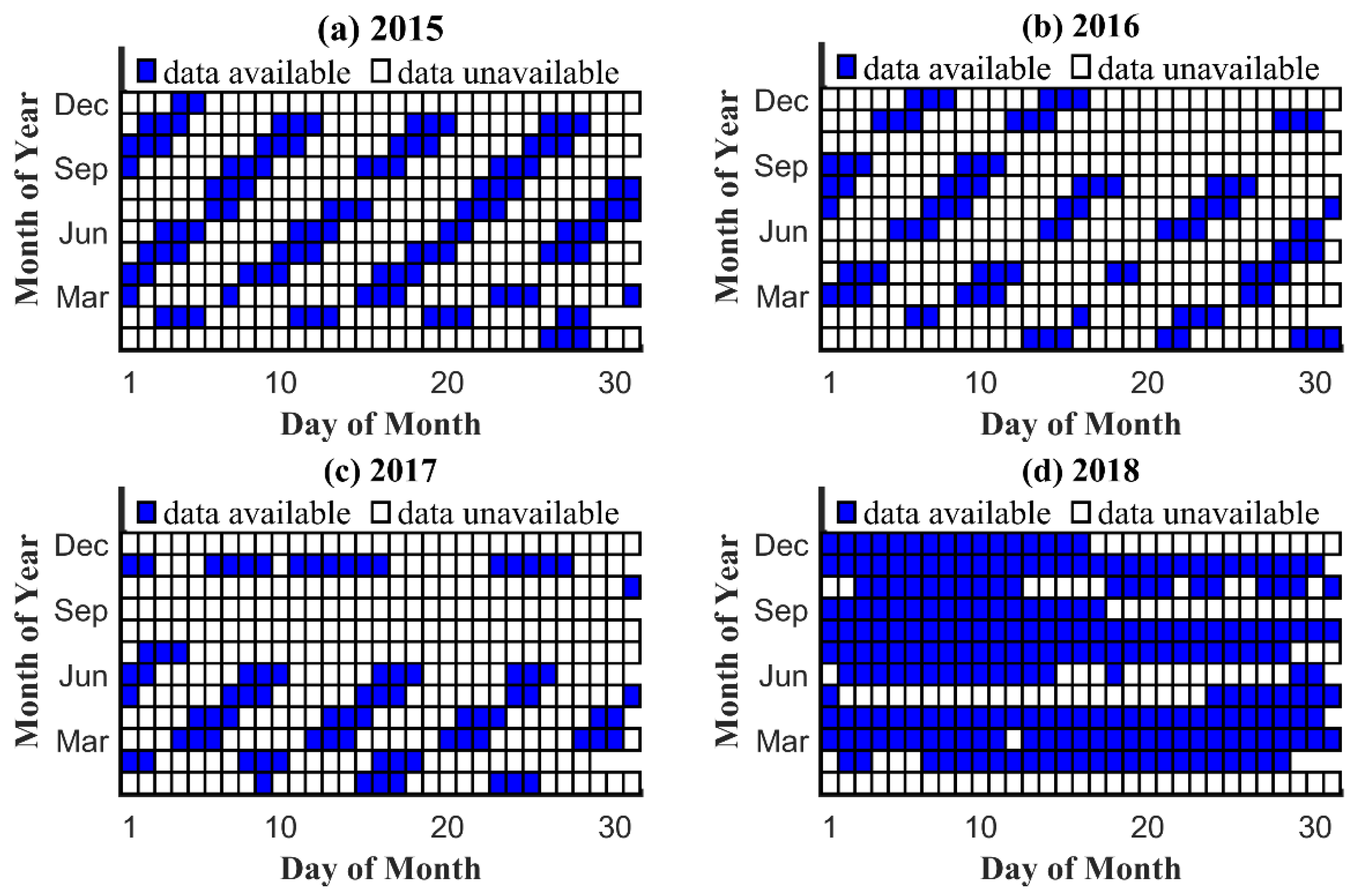
2.1. TDS-1 Mission and Datasets

Spaceborne GNSS-R data from TDS-1 include three different data processing levels, e.g., Level 0 (L0), Level 1 (L1) and Level 2 (L2) [44]. L0 mainly contains the raw data, which are not available to the public except for some sample data. L1 includes L1a and L1b, which are the data converted from the L1a onboard processed DDMs and converted to NetCDF format. The L1b release includes the DDMs and metadata used in this study. Level 2 refers to the wind speed and mean square slope products. DDMs are generated by the Space GNSS Receiver Remote Sensing Instrument (SGR-ReSI) through cross-correlating scattered signals with code replicas generated locally for different time delays and Doppler shifts. When the reflection surface is smooth, most of the scattered power comes from the specular point, and very little from the glistening zone around the specular point [45]. Compared with the sea ice surface, the one of sea water yields a non-coherent reflection with more scattering in the delay and Doppler domains. This distinct characteristic in the spreading from sea ice and water provides the opportunity to monitor sea ice.

The TDS-1 satellite was launched in July 2014 and started its data collection from September 2014. As one of eight payloads onboard on TDS-1, the SGR-ReSI took measurements two days in an eight-day cycle until 2018. The SGR-ReSI was operated in full time mode (7/7 days) during its extension from February to December 2018. The TDS-1 data provide an intense coverage over most of Arctic and Antarctic regions as the satellite runs on a quasi-Sun synchronous orbit with an altitude of ~635 km and an inclination of 98.4°. The TDS-1 data are accessible on the Measurement of Earth Reflected Radio-navigation Signals by Satellite (MERRBys, www.merrbys.co.uk). The available DDMs from TDS-1 consists of 20 Doppler shift bins with an interval of 500 Hz and 128 delay bins with a resolution of 250 ns, which is the length of 0.25 C/A code chips. Figure 1 presents two different DDMs collected over sea water and ice, respectively. It is obvious that the spreading of DDM from sea ice is much less than that of sea water. The reflection of sea ice is more coherent than that of sea water, which results in more scattering in the delay and Doppler domains due to the presence of waves on the open water surface.

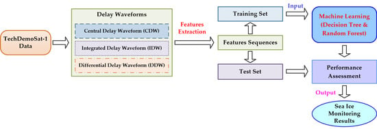
2.2. Extraction of Features

The scattering components of DDM come from the glistening zone with different delay and Doppler shifts with respect to the specular point. The method proposed in [28] uses the two-dimensional delay waveforms generated from DDMs as basic observables for easier data processing. As introduced in [28], the cross section of 20 different Doppler shifts produces 20 delay waveforms, whose summation refers to the integrated delay waveform (IDW) [25] of the DDM over the Doppler domain. The relationship between the power of scattered signals and time delay is illustrated by DDM, which is described by the model proposed in [45] based on the bistatic radar equation:

$$DDM=T_i^2{\displaystyle \int }\frac{D^2\left(\overrightarrow{\rho }\right)}{4\pi R_T^2\left(\overrightarrow{\rho }\right)R_R^2\left(\overrightarrow{\rho }\right)}{\left|\mathsf{\Lambda }\left(\mathsf{\tau }\right)\times S\left(f_D\right)\right|}^2{\sigma }_0\left(\overrightarrow{\rho }\right)d^2\rho$$

(1)

where $T_i$ represents the coherent integration time, $\mathsf{\tau }$ represents the time delay, $D^2$ represents the function of power antenna footprint, $R_T$ represents the distance from the scattering point to GNSS transmitters, $R_R$ represents the distance from the receiver to the scattering point, $\mathsf{\Lambda }$ is a triangular function as a function of time delay, S is a sinc function in the frequency domain for GPS C/A codes, ${\sigma }_0$ represents the normalized bistatic radar cross section, $f_D$ represents the Doppler shift frequency and $\rho$ represents the vector from the specular reflection point to the scattering point.

In the TDS-1 mission, the coherent integration time is 1 ms and the Doppler bandwidth can be described by $\mathsf{\Delta }{f}_0=1/2T_i$. If the maximum and minimum Doppler shift of the scattered signal is defined as $f_{max}$ and $f_{min}$, respectively, the width of the glistening zone can be described by $f_{max}-f_{min}$. If the Doppler bandwidth is larger than the width of the glistening zone (i.e., $\mathsf{\Delta }{f}_0>f_{max}-f_{min}$), the Doppler effects is negligible. The sinc function S is equal to 1 and the cross section with zero Doppler shift (Doppler = 0) is a particularly Central Delay Waveform (CDW) from the DDM. The waveform can be defined as:

$$CDW=T_i^2{\displaystyle \int }\frac{D^2\left(\overrightarrow{\rho }\right)}{4\pi R_T^2\left(\overrightarrow{\rho }\right)R_R^2\left(\overrightarrow{\rho }\right)}{\left|\mathsf{\Lambda }\left(\mathsf{\tau }\right)\right|}^2{\sigma }_0\left(\overrightarrow{\rho }\right)d^2\rho$$

(2)

Another observable termed as differential delay waveform (DDW) was used to describe the degree of difference between CDW and IDW. The DDW between normalized CDW (NCDW) and normalized IDW (NIDW) can be defined as:

$$DDW=NIDW-NCDW$$

(3)

The IDW is useful to describe the power spreading characteristics due to surface roughness. In order to extract features from DDMs, several data pre-processing schemes presented in the previous study [23,28] should be applied to subtract the noise floor to obtain normalized DDM (NDDM) with NIDW, NCDW and DDW. Contrary to the previous studies, data with a peak signal-to-noise ratio (SNR) above −3 dB are adopted to increase the amount of data. The more relaxed data filtering strategy is also useful to inspect the applicability and generality of the proposed methods.

There are no effective signals over the several starting and ending delay bins. Therefore, only a part of delay bins from chips −3 to 8.75 (48 delay bins) around the specular point are adopted to extract features. The ground tracks and parts of samples (DDMs and corresponding delay waveforms) of TDS-1 data collected over Baffin Bay on 15 January 2016 are presented in Figure 2. The open water, ice and land are filled with light blue, white and light yellow, respectively. The ground tracks of sea ice and water are depicted by magenta and blue, respectively. The DDMs of sea ice and water are presented with the area marked with cyan and green rectangle respectively. Figure 2a presents the continuous DDMs over the water-ice transition area marked with red rectangle. The corresponding delay waveforms (i.e., NCDW, NIDW and DDW) are shown in Figure 2b. As shown in Figure 2b, the shape of delay waveforms changes from water to ice surface. The largest change in delay waveforms is between DDM 487 and 488.

A few feature parameters are derived from the delay waveforms to monitor sea ice. Figure 3 presents the NCDW, NIDW and DDW, which can be divided into a left edge (LE) and right edge (RE) according to the point with a delay value of zero. The spaceborne GNSS-R DDMs are generated through cross-correlating scattered signals with code replicas generated locally for different time delays and Doppler shifts [44]. The maximum power is tracked in the Doppler domain to identify the delay value of zero. The earth surface (e.g., sea surface height fluctuations, ice height above the ellipsoid) may affect the geometry and lead to incorrect estimation. This study mainly focuses on the relative change, and not on altimetry applications. Therefore, the impacts of those factors have not been taken into consideration.

The LE is related to the area above the reflection surface, which results in its insensitivity to the characteristics of reflection surface. Only the RE-related observables are applied to monitor sea ice in this study. Six characteristic parameters termed as RE slope of CDW (RESC), RE slope of IDW (RESI), RE slope of DDW (RESD), RE waveform summation of CDW (REWC), RE waveform summation of IDW (REWI) and RE waveform summation of DDW (REWD) are extracted as features for monitoring sea ice. These features can be computed according to the equations summarized in

Table 1. The mathematical description of six selected features (i.e., RESC, RESI, RESD, REWC, REWI, REWD). RESC is the right edge slope of CDW. RESI is the right edge slope of IDW. RESD is the right edge slope of DDW. REWC is the right edge waveform summation of CDW. REWI is the right edge waveform summation of IDW. REWD is the right edge waveform summation of DDW.

Features	Mathematical Description
RESC	$\left({\displaystyle \sum }_{i=1}^n{\tau }_i{C}_i^R-n\overline{\tau }\overline{C^R}\right)/\left({\displaystyle \sum }_{i=1}^n{\tau }_i^2-n{\overline{\tau }}^2\right)$
RESI	$\left({\displaystyle \sum }_{i=1}^n{\tau }_i{I}_i^R-n\overline{\tau }\overline{I^R}\right)/\left({\displaystyle \sum }_{i=1}^n{\tau }_i^2-n{\overline{\tau }}^2\right)$
RESD	$\left({\displaystyle \sum }_{i=1}^n{\tau }_i{D}_i^R-n\overline{\tau }\overline{D^R}\right)/\left({\displaystyle \sum }_{i=1}^n{\tau }_i^2-n{\overline{\tau }}^2\right)$
REWC	${\displaystyle \sum }_{i=1}^n{C}_i^R$
REWI	${\displaystyle \sum }_{i=1}^n{I}_i^R$
REWD	${\displaystyle \sum }_{i=1}^n{D}_i^R$

.

In the equations in Table 1, n ($n\ge 2$) is the number of delay bins for curve fitting and 1 delay bins is equal to 0.25 chips; ${\tau }_i$ is the time delay value of the ith point; $C_i^R$, $I_i^R$ and $D_i^R$ are the waveform values of right edge of CDW, IDW and DDW, respectively; $\overline{C^R}$, $\overline{I^R}$ and $\overline{D^R}$ are the mean waveform values of points applied for fitting of CDW, IDW and DDW, respectively; $\overline{\tau }$ is the mean of time delay of points applied for fitting. n is set as 5 for RESC, RESI and RESD and 7 for REWC, REWI and REWD.

2.3. Validation Data

Two sea ice datasets are used to evaluate the performance of the proposed sea ice monitoring approach. The sea ice edge (SIE) data provided by the Ocean and Sea Ice Satellite Application Facility (OSISAF) are used as the reference data [46,47]. The OSISAF SIE data is generated with a grid resolution of 10 km using a Bayesian approach based on the combination of ASCAT (Advanced Scatterometer) and SSMIS (Special Sensor Microwave Imager Sounder) data with different channels (e.g., 19, 37 and 91 GHz). It is worth noting that the OSISAF data has quality flags which indicate the quality of the sea ice products. The data are divided into five levels according to the confidence levels. The confidence level of 0 means unprocessed, 1 means erroneous, 2 means unreliable, 3 means acceptable, 4 means good and 5 means excellent. The data with a minimum confidence data level of 3 are adopted in this study [46].

The sea ice concentration (SIC) data generated through the Arctic radiation and the turbulence interaction study Sea Ice (ASI) algorithm using AMSR-2 (Advanced Microwave Space Radiometer-2) data are also used as the reference data [4]. This SIC map was obtained from the online sea ice data platform www.meereisportal.de [48]. The reference SIC data are used to generate daily maps in the polar stereographic coordinates with a grid resolution of 6.25 km. The TDS-1 DDMs can be matched with the SIC maps using the location of specular point and date of data collection, which are contained in the data Level 1b. The DDM with a SIC value above 15% is regarded as sea ice, otherwise as sea water [25].

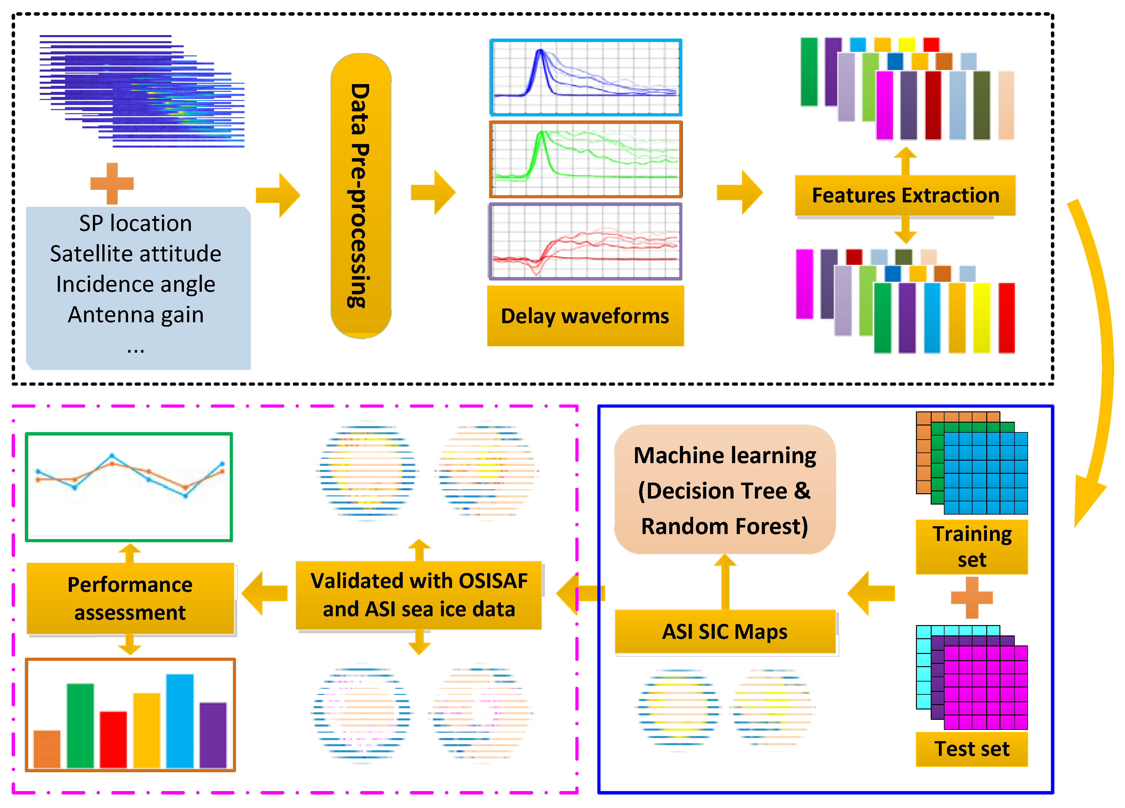
2.4. Machine Learning-Aided Sea Ice Monitoring Methods

One of the most important tasks of monitoring sea ice is to distinguish sea ice from water. Therefore, the problem of this study can be regarded as a typical binary classification that can be done by using an ML method on a big dataset. The process flow of monitoring sea ice using ML is presented in Figure 4.

The ML-based sea ice monitoring method includes three steps: (1) feature extraction from the TDS-1 data; (2) the learning process with the training dataset using ML algorithms; (3) the automatic discrimination between data collection over sea ice and over water. A total of seven input variables are used, which are the reference SIC maps and the sequence of six features (i.e., RESC, RESI, RESD, REWC, REWI and REWD) extracted from the TDS-1 data. When the reflection is coherent, the footprint of the TDS-1 DDM is about 6 km by 0.4 km along the track and across track, respectively [25,26,30], which is comparable with the reference SIC maps with a grid resolution of 6.25 km. The footprint is much larger for incoherent reflections. The specular point of each DDM is used to match the reference data. In general, the ML is based on two different data sets (training-set and test-set). The training data are pre-labeled using the reference SIC map; thus, the relationship between input parameters and output results can be modeled using suitable ML algorithms. Then, the output results of test data can be obtained using the pre-built model. According to the process of building models, machine learning could be mainly categorized into supervised learning, unsupervised learning and semi-supervised learning. The characteristics of supervised learning is that training data have priori information (results). In this study, the task is to distinguish sea ice from water and the output results of training datasets can be obtained through the reference SIC data. Therefore, two types of supervised learning—DT and RF—are adopted to monitor sea ice.

2.4.1. Decision Tree Algorithm

Decision tree (DT) is one of the simplest and most useful algorithms for classification [49,50]. It has been used to various remote sensing applications [51,52,53]. The structure of a decision tree is constructed upside down with three parts: internal node, branches and leaf. The first internal node is called the root, where classification starts. The internal node stands for a condition that is expressed by the feature parameters. Based on the node, the decision tree splits into branches according to a discriminant function. The tree ends at the leaf, which represents a final classification decision. Distinguishing between sea ice and water can be regarded as a binary classification problem. Thus, the algorithm C4.5 [54] is used, which recursively splits training data into subdivisions using a set of attributes described by input variables. C4.5 builds decision trees from a set of training data using the concept of information entropy. The training data are a set $S=s_1,s_2,\dots s_i$ of already classified samples. Each sample $s_i$ consists of a p-dimensional vector $\left(x_{1,i},x_{2,i},\dots ,x_{p,i}\right)$, where the $x_i$ values represent attribute values or features of the sample, as well as the class in which $s_i$ falls. C4.5 uses the information gain ratio to construct a decision tree. The information gain ratio is defined as:

$$G_{ratio}=\frac{\left[{{\displaystyle \sum }}_{k=1}^{m}p\left(k\right)lo{g}_{2}p\left(k\right)+{{\displaystyle \sum }}_{j=1}^v\left(\left|D_j\right|/\left|D\right|\right)Ent\left(D_j\right)\right]}{{{\displaystyle \sum }}_{j=1}^v\left(\left|D_j\right|/\left|D\right|\right)lo{g}_2\left(\left|D_j\right|/\left|D\right|\right)}$$

(4)

where $m$ is the number of categories; $v$ is the number of selected features; $D$ is the number of samples; $D_j$ is the jth sample. In this paper, only two categories, i.e., sea ice and sea water, are included, so $m=2$. As six features are selected, $v$ is equal to 6. The information gain ratio can be simplified as:

$$G_{ratio}=\frac{\left[{{\displaystyle \sum }}_{k=1}^{2}p\left(k\right)lo{g}_{2}p\left(k\right)+{{\displaystyle \sum }}_{j=1}^6\left(\left|D_j\right|/\left|D\right|\right)Ent\left(D_j\right)\right]}{{{\displaystyle \sum }}_{j=1}^6\left(\left|D_j\right|/\left|D\right|\right)lo{g}_2\left(\left|D_j\right|/\left|D\right|\right)}$$

(5)

C4.5 has several advantages. It can mitigate overfitting through single pass pruning process, handle both discrete and continuous data and address the problem of incomplete data, which is common in practical applications.

2.4.2. Random Forest algorithm

Another ensemble learning method for classification is random forest (RF), which constructs a collection of DT at training time. RF combines a boosting sampling strategy and Classification and Regression Tree (CART) to overcome the drawback of a single CART, such as overfitting problems. CART uses a Gini index [55] to measure the impurity of training datasets, while C4.5 utilizes the concept of entropy. The Gini index is described by:

$$G_{index}\left(p\right)=1-{{\displaystyle \sum }}_{l=1}^s{p}_l^2$$

(6)

where s is the number of categories and $p_l$ is the proportion of samples belonging to class l. Since sea ice monitoring is a binary classification problem. Thus, the Gini index can be simplified as:

$$G_{index}\left(p\right)=2p\left(1-p\right)$$

(7)

where p can be regarded as the probability that samples belong to sea ice.

The advantages of CART include that the rules can be interpreted easily and that it provides automatic processing of parameters selection, data missing, outliers, variable interaction and nonlinear relationships. However, one of the biggest shortcomings of a single CART is overfitting. The strategy of bagging can effectively solve the problem through constructing a large number of independent trees and reduce errors that may be caused by some unstable classifiers [56]. Due to its advantages, RF shows great potential in many remote sensing applications [57].

3. Results

The TDS-1 data collected over the Arctic and Antarctic regions with the latitude above 55°N and 55°S from January 2015 to December 2018 are analyzed in this study. Twenty percent of the data is randomly selected to train the ML-based models to distinguish sea ice from water. The remaining 80% of data is used as the test dataset to validate the sea ice monitoring methods developed using ML algorithms.

As aforementioned, the GNSS-R receiver on the TDS-1 satellite was not always in operation. Thus, the TDS-1 data are not accessible every day. Figure 5 presents the situation of data availability from January 2015 to December 2018. The data unavailability from August to October 2017 is probably due to the scheduled shutdown of TDS-1 mission, which was originally set to the end of July 2017. In fact, the TDS-1 mission was extended from February to December 2018. During its extension, the SGR-ReSI was operated every day, rather than the two of eight-day cycle as in the first three years. The coverage and sampling were increased by a factor of four. The data missing for a few days in 2018 may result from statutory holidays, such as Christmas.

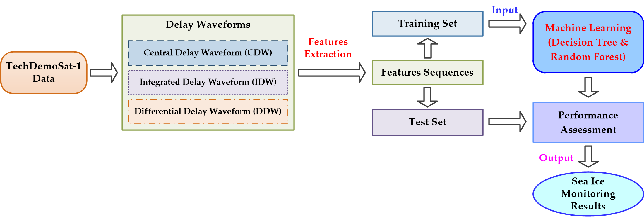
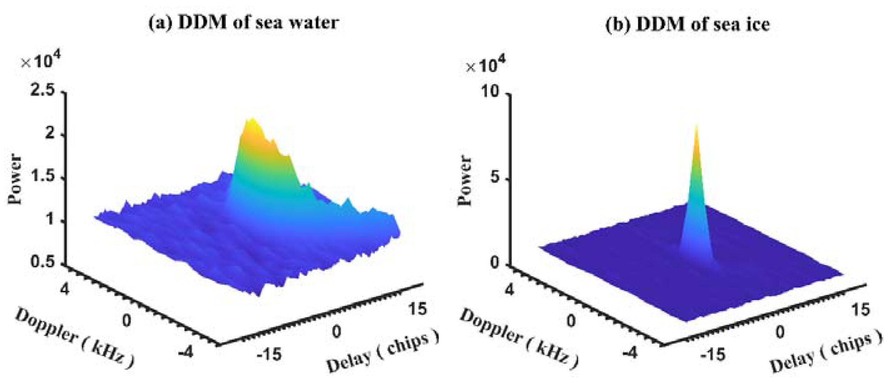
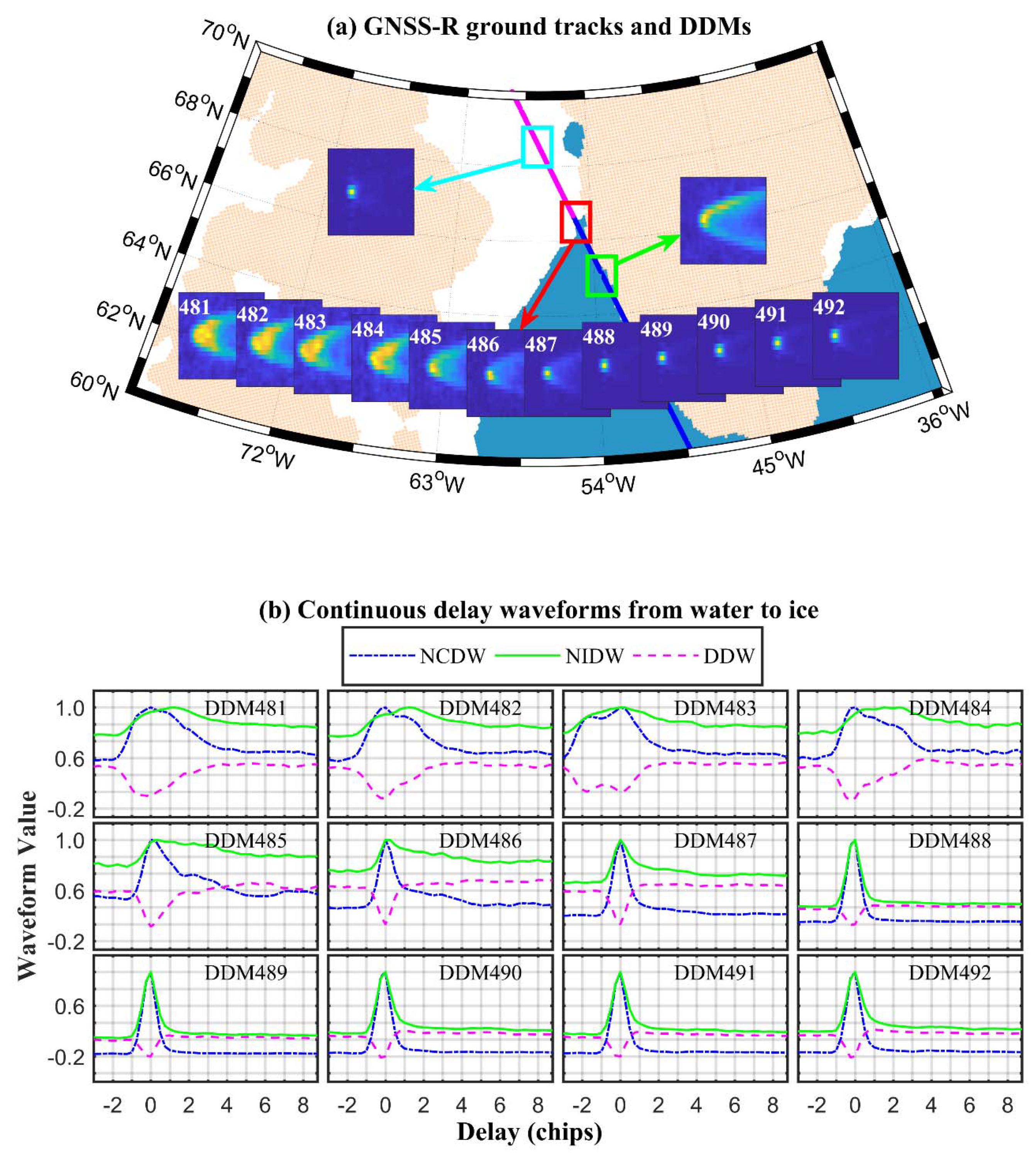
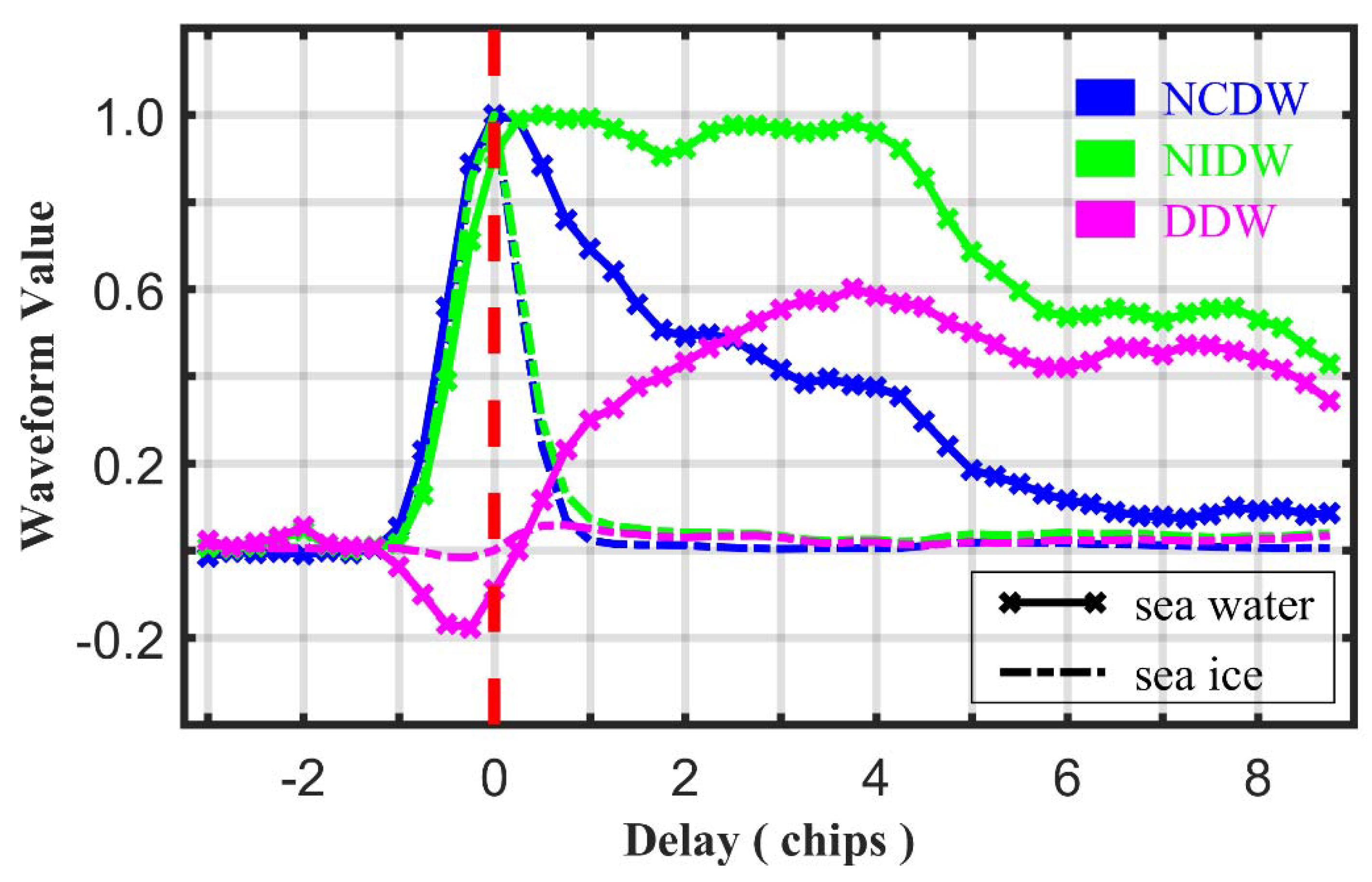
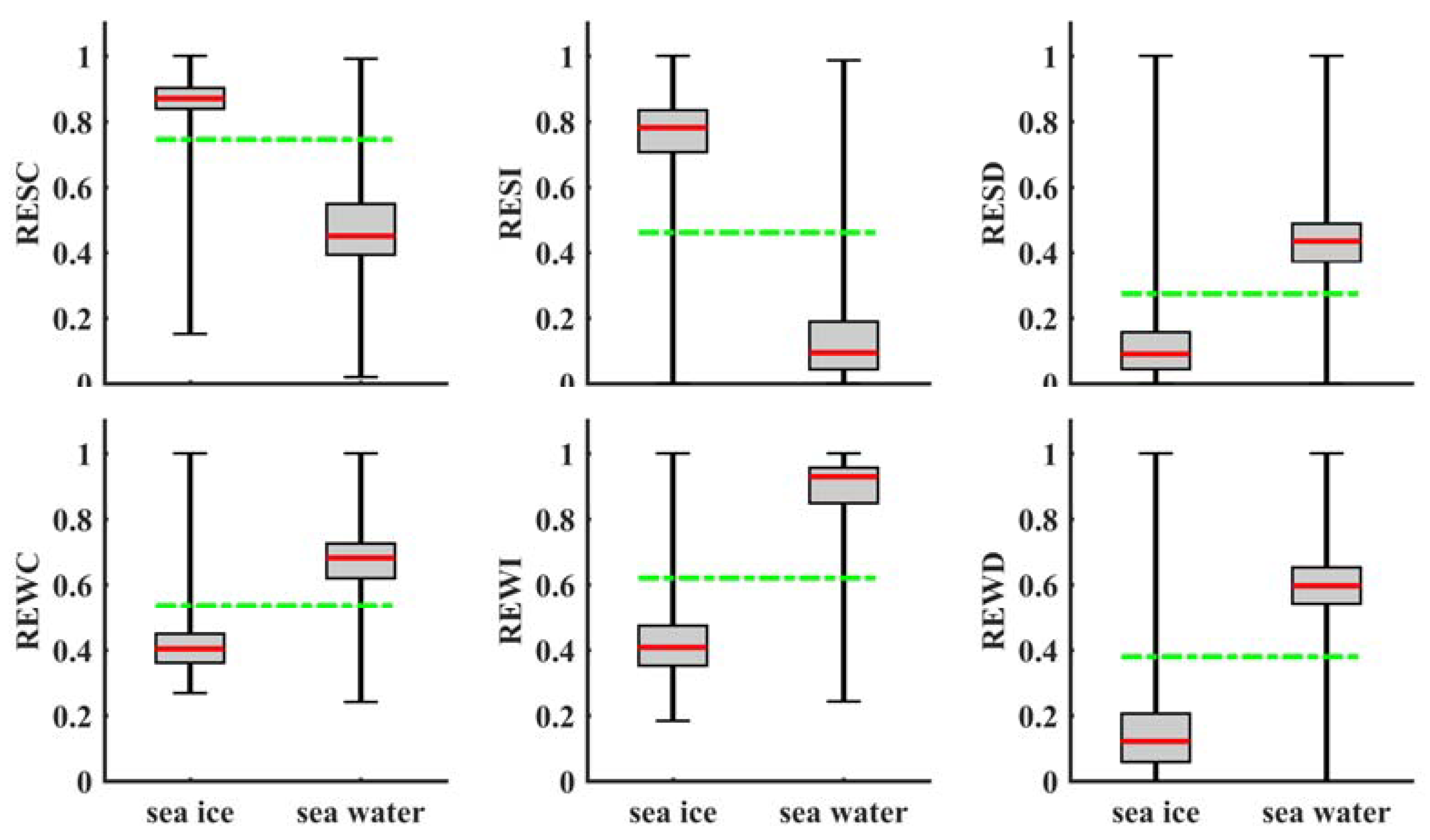
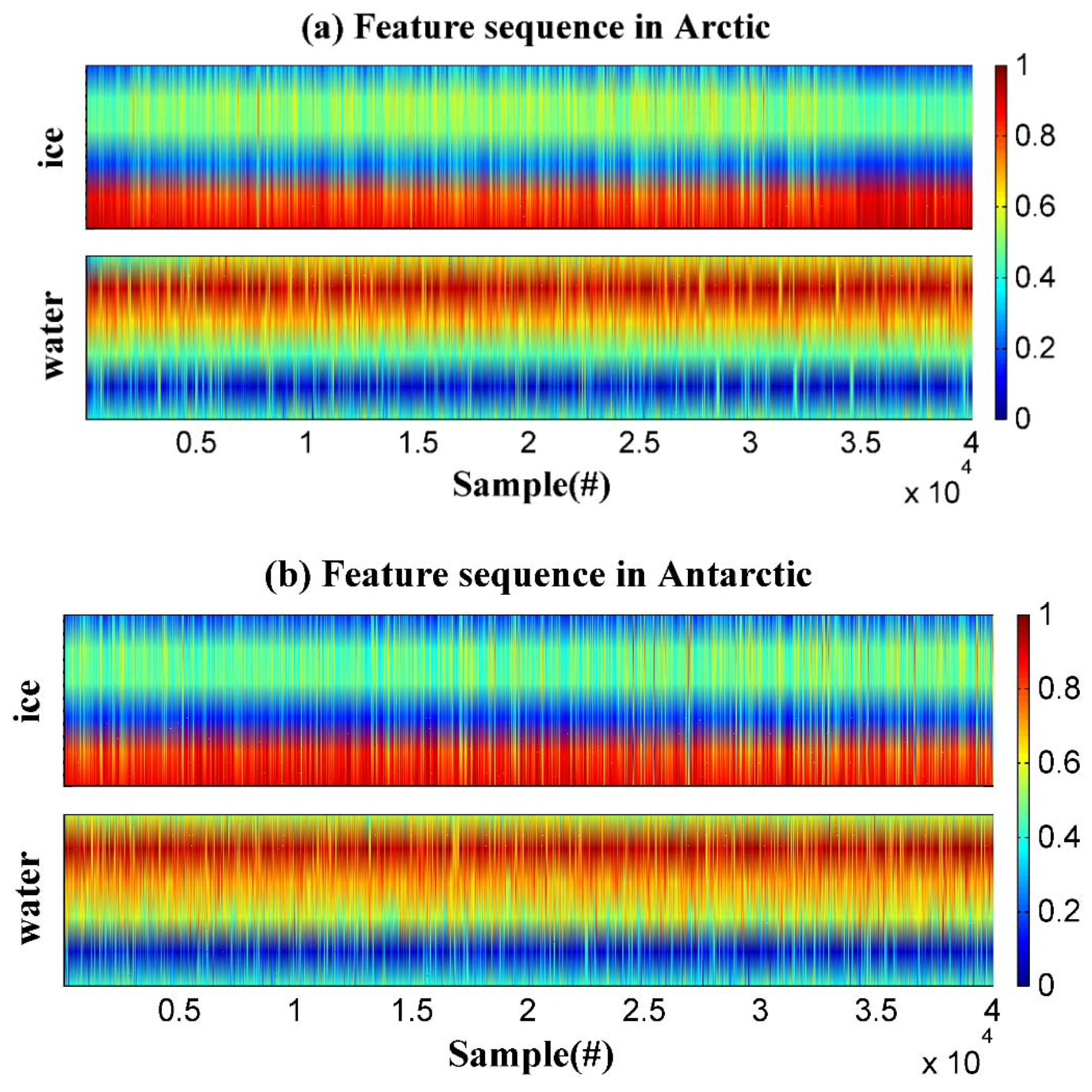
3.1. Characteristics of GNSS-R Features

The distribution characteristics of six feature parameters (RESC, RESI, RESD, REWC, REWI and REWD) for sea ice and water are shown in Figure 6. The vertical height of the boxes represents the interquartile range of the samples, while the parallel line depicted in red inside the boxes is the median value of the samples for each feature. The green dotted line represents the threshold obtained by the method proposed in [28] for distinguishing sea ice from water. It is clear that sea ice shows a distinct difference between sea water for all the features considered. This is because the reflection over the sea ice surface is usually more coherent. The sea water surface is often rougher than that of sea ice and easily affected by ocean winds, which results in wider scattering. The median values of each parameter for sea ice and water are significantly different. However, the distribution of features of sea ice and water is more or less overlapped. As shown in Figure 6a, the RESC values of sea ice range from 0.15 to 1 and those of sea water range from 0.02 to 0.99; the threshold is 0.745. If RESC < 0.745, it is regarded as sea water; if RESC > 0.745, it is regarded as sea ice. However, some points of RESC below 0.745 appear in sea ice, and some points above 0.745 appear in sea water; these points are overlap. This indicates that simple thresholding of each feature may result in some false discrimination between sea ice and water.

This study uses the combination of six features derived from the delay waveforms of different Doppler spread characteristics to describe the characteristics of reflecting surface. The six features of samples are composited into sequences, which are applied as input variables to train the sea ice monitoring model. The six features are combined into sequences in order. RESC, RESI, RESD, REWC, REWI and REWD values are presented from bottom to top in the y-axis. The feature sequences of samples in the Arctic and Antarctic regions are presented in Figure 7.

As shown in Figure 7a,b, the feature sequences of 40,000 samples for sea ice (upper plot) and water (lower plot) show distinct differences, which provide the opportunities of monitoring sea ice. Moreover, the feature sequences can describe the characteristics more accurately than individual features.

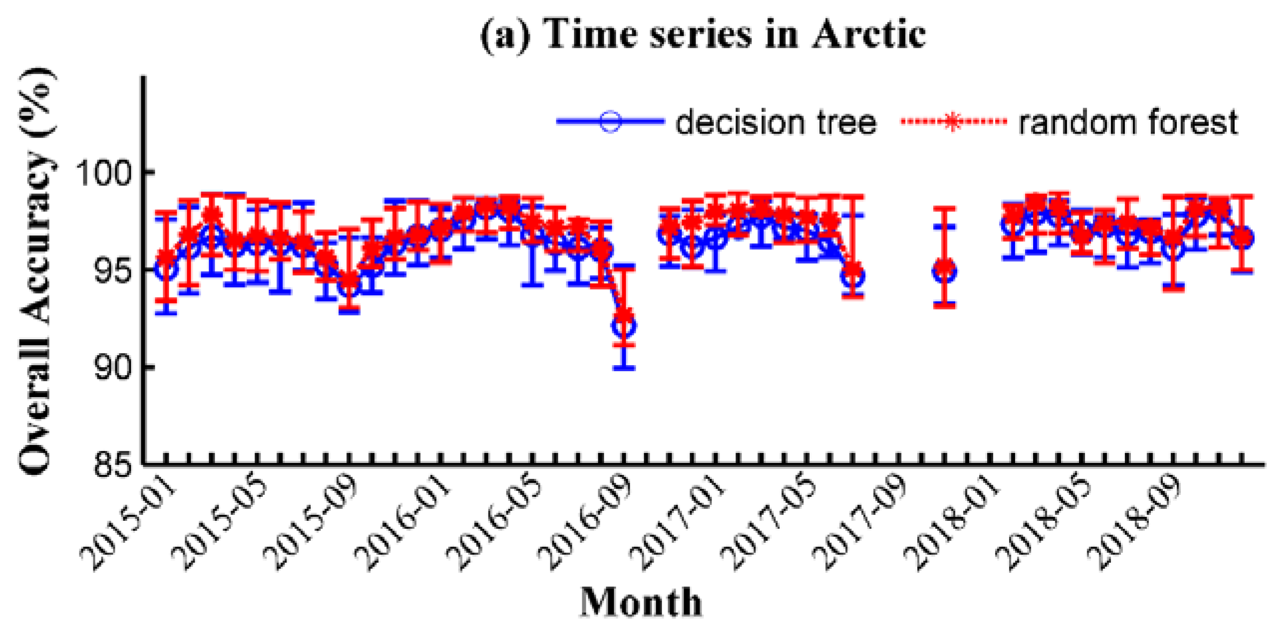
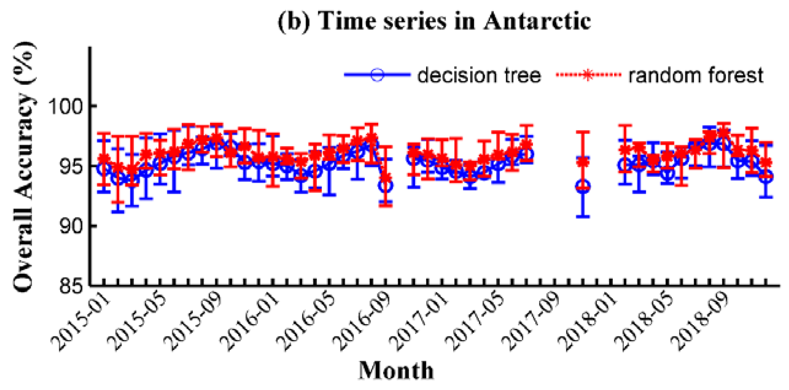
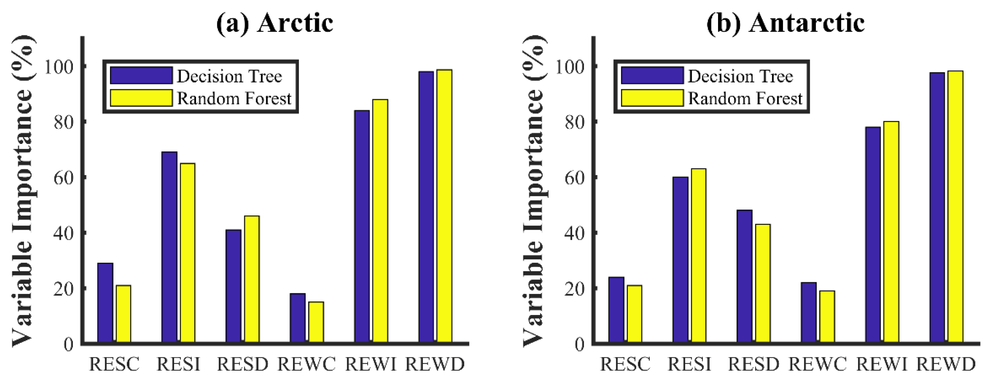
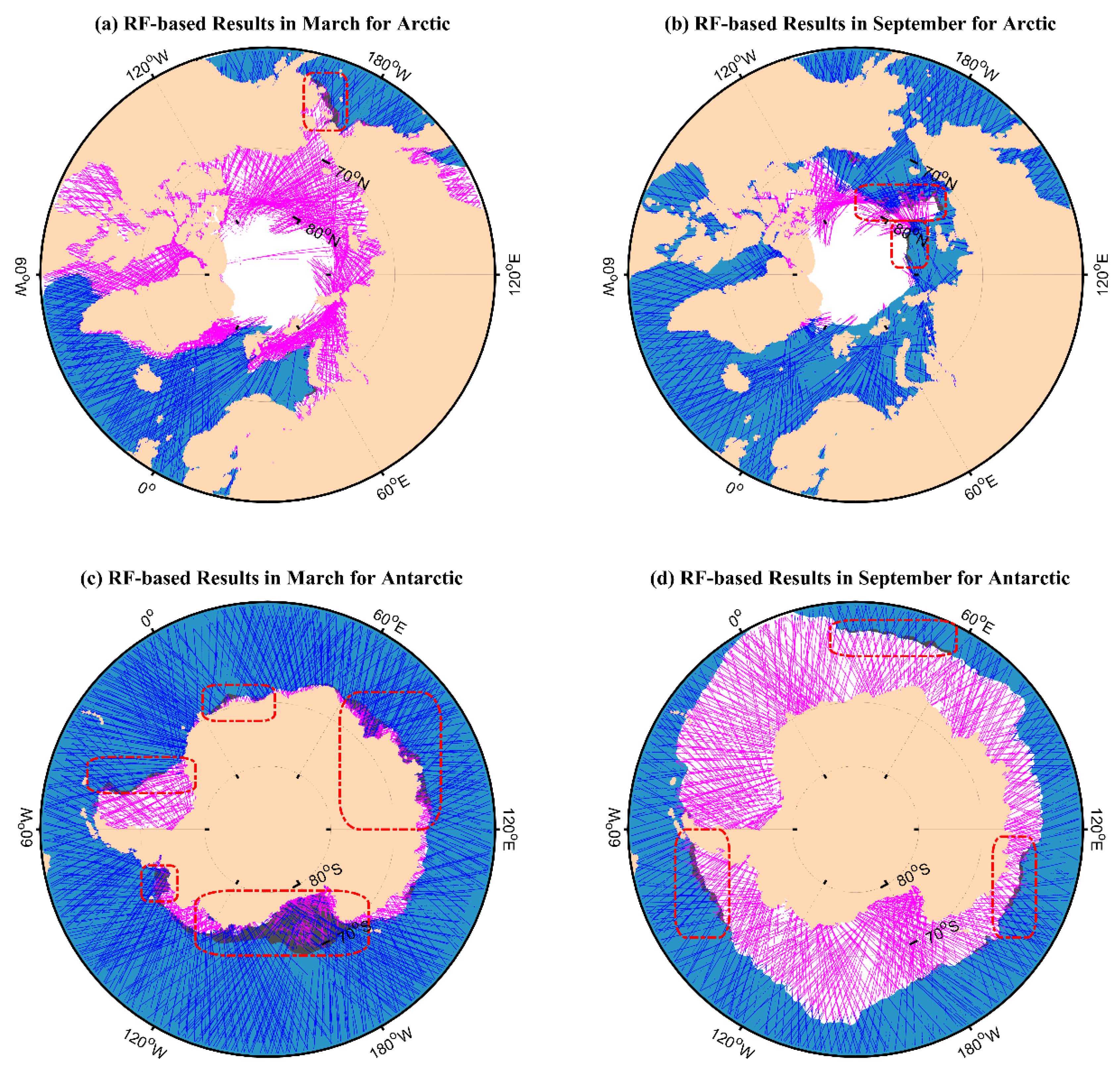
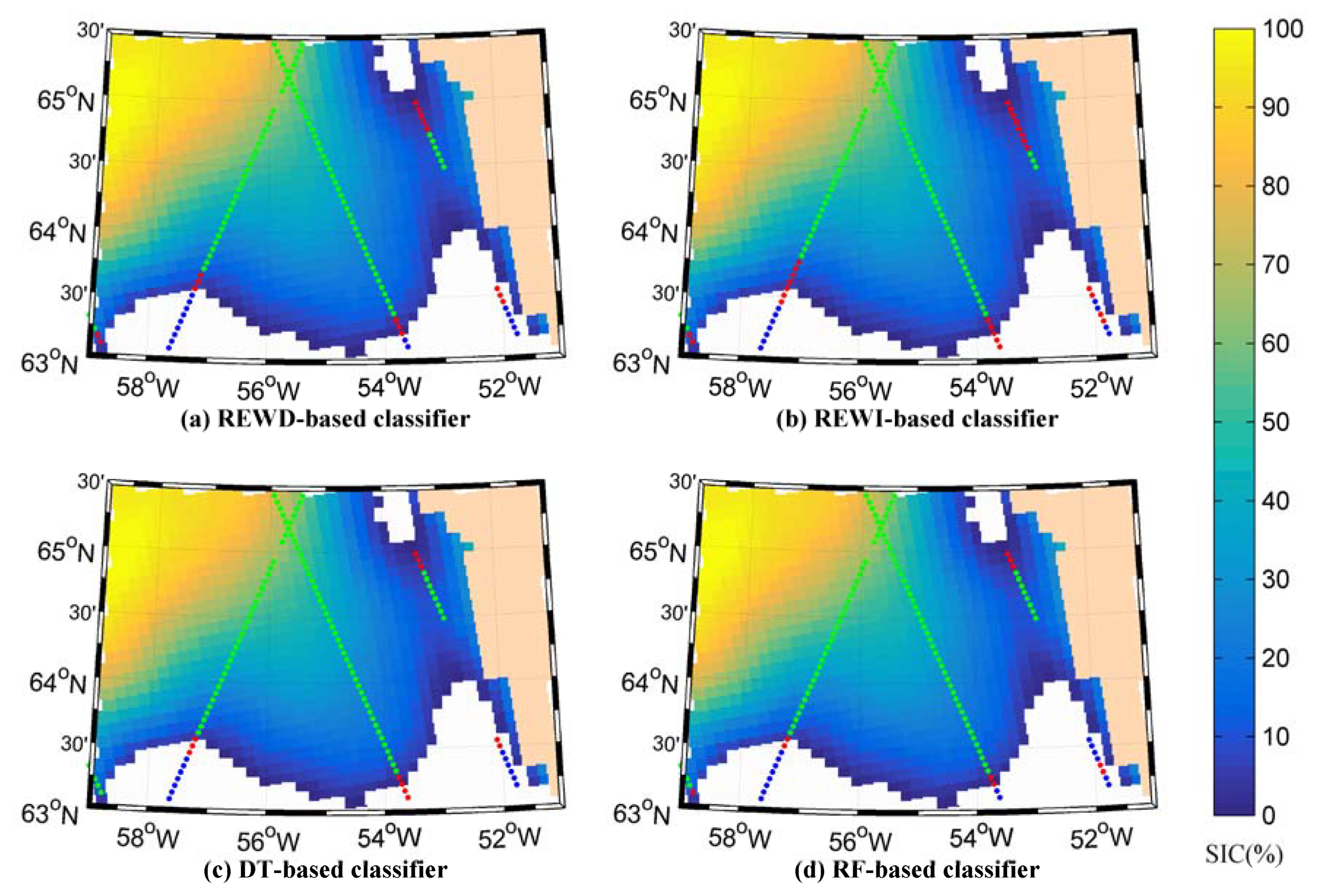
3.2. Sea Ice Monitoring Performance

The sea ice monitoring models based on DT and RF algorithms are quantitatively assessed using confusion matrices [58] through a comparison with the OSISAF SIE data using the test data. In the field of machine learning and specifically the problem of statistical classification, a confusion matrix [56], also known as an error matrix, is a specific table layout that allows visualization of the performance of a supervised learning algorithm. The confusion matrix is a table with two rows and two columns that reports the number of false positives, false negatives, true positives and true negatives. The error matrices, overall accuracy and kappa coefficient [59] of the agreement are used as indicators to evaluate the performance of the DT and RF models. The performance of the DT and RF models for the Arctic and Antarctic regions are presented in

Table 2. The confusion matrix for the decision tree (DT) algorithm using data from Arctic and Antarctic regions.

Arctic	Reference classified as	Sea ice	Sea water	Sum	User accuracy
	Sea ice	1,242,947	6513	1,249,460	99.48%
	Sea water	61,677	1,427,415	1,489,092	95.86%
	Sum	1,304,624	1,433,928	2,738,552
	Producer accuracy	95.27%	99.55%
	Overall accuracy			97.51%
	Kappa coefficient			95.00%
Antarctic	Reference classified as	Sea ice	Sea water	Sum	User accuracy
	Sea ice	1,368,301	29,491	1,397,792	97.89%
	Sea water	110,509	1,572,579	1,683,088	93.43%
	Sum	1,478,810	1,602,070	3,080,880
	Producer accuracy	92.53%	98.16%
	Overall accuracy			95.46%
	Kappa coefficient			90.88%

and

Table 3. The confusion matrix for the Random Forest (RF) algorithm using data from Arctic and Antarctic regions.

Arctic	Reference classified as	Sea ice	Sea water	Sum	User accuracy
	Sea ice	1,275,679	25,121	1,300,800	98.07%
	Sea water	28,945	1,408,807	1,437,752	97.99%
	Sum	1,304,624	1,433,928	2,738,552
	Producer accuracy	97.78%	98.25%
	Overall accuracy			98.03%
	Kappa coefficient			96.04%
Antarctic	Reference classified as	Sea ice	Sea water	Sum	User accuracy
	Sea ice	1,411,677	57,411	1,469,088	96.09%
	Sea water	67,133	1,544,659	1,611,792	95.83%
	Sum	1,478,810	1,602,070	3,080,880
	Producer accuracy	95.46%	96.42%
	Overall accuracy			95.96%
	Kappa coefficient			91.90%

, respectively.

The overall accuracy of DT model is 97.51% and 95.46% for the Arctic and Antarctic, respectively, while the RF model produced an overall accuracy of 98.03% and 95.96% for the Arctic and Antarctic, respectively. The producer and user accuracies of sea water are higher than those of sea ice for both models. This may be because the sea ice with a low SIC is more easily misidentified as sea water. When the surface area with both ice and water is driven by wind field, the surface will become rougher, and the sea ice surface is recognized as sea water. Although the DT and RF models obtain similar overall accuracies, the Kappa coefficient of agreement of RF model is slightly higher than that of DT, which indicates that the performance of the RF algorithm is better than that of DT. Although the overall accuracy obtained in this study is slightly lower than that in the previous study, the dataset used here is much larger and the data filter requirement is lower. This indicates the method developed and applied here is of better applicability and generality. When using data only from the initial mission, as we did in our previous study [25], the overall accuracy of this method is 0.22% better than the REWD method we applied there.

The previous study [37] indicated that the support vector machine (SVM) outperforms the neural network (NN) and convolutional neural network (CNN) methods for detecting sea ice using spaceborne GNSS-R data. SVMs are capable of operating classification tasks by finding a hyperplane that can best distinguish (with the maximum margin) between different types. NNs are extremely flexible in the types of data they can support. NNs do a decent job at learning the important features from basically any data structure, without having to manually derive features. CNNs are much less flexible models compared to a fully connected network, and are biased toward performing well on image. In order to evaluate the performance of proposed methods, the SVM is adopted for comparison. The sea ice monitoring results obtained by SVM based methods are shown in

Table 4. The confusion matrix for the Support Vector Machine (SVM) algorithm using data from Arctic and Antarctic regions.

Arctic	Reference classified as	Sea ice	Sea water	Sum	User accuracy
	Sea ice	1,270,679	31,121	1,301,800	97.61%
	Sea water	33,945	1,402,807	1,436,752	97.64%
	Sum	1,304,624	1,433,928	2,738,552
	Producer accuracy	97.40%	97.83%
	Overall accuracy			97.62%
	Kappa coefficient			95.24%
Antarctic	Reference classified as	Sea ice	Sea water	Sum	User accuracy
	Sea ice	1,406,997	63,331	1,470,328	95.69%
	Sea water	71,813	1,538,739	1,610,552	95.54%
	Sum	1,478,810	1,602,070	3,080,880
	Producer accuracy	95.14%	96.05%
	Overall accuracy			95.61%
	Kappa coefficient			91.21%

. The proposed RF-based sea ice monitoring approach shows better accuracy than the SVM-based method, while the SVM-based sea ice monitoring scheme outperforms the DT-based one. The feature sequences applied in this study are extracted from delay waveforms (NCDW, NIDW and DDW) with different doppler shifts.

4. Discussion

For further analysis, the time series of overall accuracy of sea ice monitoring is computed using all the available data from January 2015 to December 2018 (Figure 8). The overall accuracy of the Arctic region is significantly lower in September 2016 since the sea ice melts in this season, while the changing trend of the Antarctic region is reverse as the seasonal alternation between the Arctic and Antarctic is opposite.

To analyze the impact of each variable, the relative importance of variables for sea ice monitoring is shown in Figure 9. REWD is used at all nodes in the DT algorithm, which results in a relatively high contribution to sea ice monitoring. REWI is useful as it can be used to distinguish sea ice from water with very low error. The REWD is the most important parameter, followed by REWI, RESI, RESD, RESC and REWC in the DT algorithm. Like the DT algorithm, REWC is of the least significance for monitoring sea ice in the RF algorithm.

The RF-based GNSS-R sea ice monitoring results in March and September 2018 are mapped with the OSISAF SIE data in Figure 10. The white and dark gray edge (partly marked by a rounded rectangle with a red dotted line) represent the minimum and maximum ice extent for March and September in 2018, respectively. In March, the sea ice extent of Arctic region reaches the minimum and maximum on 6 and 14 March, respectively, while the minimum and maximum sea ice extent of Antarctic region appear on 1 and 31 March respectively. As shown in Figure 5d, the data are not available every day in September 2018. From 1 to 17 September, the maximum and minimum sea ice extent of Arctic region occur on 2 and 17 September, respectively, while the sea ice extent of Antarctic region reaches the minimum and maximum on 13 and 17 September, respectively. The scatter points are ground tracks of TDS-1 data with the peak SNR above −3 dB, which results in some gaps in the GNSS-R ground-tracks. In the figures, the presence of sea ice monitored using GNSS-R is illustrated by magenta points, whereas the presence of GNSS-R sea water is depicted by the blue points. As shown in Figure 10b,c, the detected sea ice and water overlaps in some areas. This is because the GNSS-R data span over one month and the ice extent changes rapidly during the melting season in the Arctic and Antarctic regions respectively.

The examples of monitoring sea ice around Greenland using four different methods are presented in Figure 11. The sea ice monitoring results are compared with the ASI SIC data. Two simple thresholding methods based on REWD (i.e., REWD > 0.38 for sea water and REWD < 0.38 for sea ice) and REWI (i.e., REWD > 0.62 for sea water and REWD < 0.62 for sea ice) used in [28] are adopted to monitor sea ice (Figure 11a,b). The simple thresholding methods result in some false monitoring of sea ice; sea ice is identified as sea water or sea water is regarded as sea ice. Although REWD and REWI are considered as useful parameters for distinguishing sea ice from water, simple thresholding based on just one parameter was shown to be insufficient for effectively monitoring sea ice. The results of DT- and RF-based approaches are presented in Figure 11c,d, respectively. The false sea ice monitoring of DT- and RF-based methods mainly appear around the sea ice edge areas with a relatively low SIC. The area with a low SIC may be affected by ocean winds, which results in a rougher surface. Then, the sea ice is wrongly identified as sea water. The effects of ocean winds on low SIC have not been analyzed in this study.

5. Conclusions

In this study, two machine learning-aided GNSS-R methods have been proposed to monitor sea ice using 42 months of TDS-1 data. The sea ice monitoring results are validated with the SIE data from OSISAF. The results showed that the proposed approach successfully distinguishes sea ice from water. The proposed RF- and DT-based sea ice monitoring approaches achieve an overall accuracy of 98.03% and 97.51%, respectively, in the Arctic regions, and 95.96% and 95.46%, respectively, in the Antarctic regions. Another ML-based method (i.e., SVM) used in the previous study [40] is also applied for comparison in this study. The SVM-based method achieves an overall accuracy of 97.62% and 95.61%, respectively, in the Arctic and Antarctic regions with the dataset used in this study.

A total of six features were combined to monitor sea ice, including RESC, RESI, RESD, REWC, REWI and REWD. Although these features have been applied to sense sea ice individually in the previous study, the combination of these six features is firstly adopted to monitor sea ice. Compared to the single observable method, the feature sequences can represent the characteristics of reflecting surface more accurately. Therefore, the ML-based approaches achieve higher accuracies than the single observable thresholding method. It would be worth noting that the input features to ML-based methods are different from the single observable thresholding method. Moreover, the spaceborne GNSS-R dataset used here spans 42 months of the TDS-1 mission, which is larger than those applied in the previous studies. The results from this study are encouraging for the GNSS-R applications of machine learning algorithms. Further research on the effects of oceans winds in the low SIC regions will benefit monitoring sea ice. In addition, the combination of multiple ML-based methods (e.g., DT, RF and SVM) will be explored in our future work.

References

1. Screen, J.A.; Simmonds, I. The central role of diminishing sea ice in recent Arctic temperature amplification. Nat. Cell Biol. 2010, 464, 1334–1337. [Google Scholar] [CrossRef] [Green Version]
2. Leisti, H.; Riska, K.; Heiler, I.; Eriksson, P.; Haapala, J. A method for observing compression in sea ice fields using IceCam. Cold Reg. Sci. Technol. 2009, 59, 65–77. [Google Scholar] [CrossRef]
3. Rae, J.; Hewitt, H.; Keen, A.; Ridley, J.; Edwards, J.; Harris, C. A sensitivity study of the sea ice simulation in the global coupled climate model, HadGEM3. Ocean Model. 2014, 74, 60–76. [Google Scholar] [CrossRef]
4. Spreen, G.; Kaleschke, L.; Heygster, G. Sea ice remote sensing using AMSR-E 89-GHz channels. J. Geophys. Res. Space Phys. 2008, 113, 113. [Google Scholar] [CrossRef] [Green Version]
5. Cardellach, E.; Rius, A.; Martin-Neira, M.; Fabra, F.; Nogues-Correig, O.; Ribo, S.; Kainulainen, J.; Camps, A.; D’Addio, S. Consolidating the Precision of Interferometric GNSS-R Ocean Altimetry Using Airborne Experimental Data. IEEE Trans. Geosci. Remote Sens. 2014, 52, 4992–5004. [Google Scholar] [CrossRef]
6. Liu, Y.; Collett, I.; Morton, Y.T.J. Application of Neural Network to GNSS-R Wind Speed Retrieval. IEEE Trans. Geosci. Remote Sens. 2019, 57, 9756–9766. [Google Scholar] [CrossRef]
7. Zhang, G.; Yang, D.; Yu, Y.; Wang, F. Wind Direction Retrieval Using Spaceborne GNSS-R in Nonspecular Geometry. IEEE J. Sel. Top. Appl. Earth Obs. Remote Sens. 2020, 13, 649–658. [Google Scholar] [CrossRef]
8. Guan, D.; Park, H.; Camps, A.; Wang, Y.; Onrubia, R.; Querol, J.; Pascual, D. Wind Direction Signatures in GNSS-R Observables from Space. Remote Sens. 2018, 10, 198. [Google Scholar] [CrossRef] [Green Version]
9. Yu, K. Weak Tsunami Detection Using GNSS-R-Based Sea Surface Height Measurement. IEEE Trans. Geosci. Remote Sens. 2015, 54, 1363–1375. [Google Scholar] [CrossRef]
10. Yan, Q.; Huang, W. Tsunami Detection and Parameter Estimation From GNSS-R Delay-Doppler Map. IEEE J. Sel. Top. Appl. Earth Obs. Remote Sens. 2016, 9, 4650–4659. [Google Scholar] [CrossRef]
11. Camps, A.; Park, H.; Pablos, M.; Foti, G.; Gommenginger, C.; Liu, P.-W.; Judge, J. Sensitivity of GNSS-R Spaceborne Observations to Soil Moisture and Vegetation. IEEE J. Sel. Top. Appl. Earth Obs. Remote Sens. 2016, 9, 4730–4742. [Google Scholar] [CrossRef] [Green Version]
12. Li, C.; Huang, W.; Gleason, S. Dual Antenna Space-Based GNSS-R Ocean Surface Mapping: Oil Slick and Tropical Cyclone Sensing. IEEE J. Sel. Top. Appl. Earth Obs. Remote Sens. 2014, 8, 425–435. [Google Scholar] [CrossRef]
13. Valencia-Domènech, E.; Camps, A.; Rodriguez-Alvarez, N.; Park, H.; Ramos-Perez, I. Using GNSS-R Imaging of the Ocean Surface for Oil Slick Detection. IEEE J. Sel. Top. Appl. Earth Obs. Remote Sens. 2012, 6, 217–223. [Google Scholar] [CrossRef]
14. Wickert, J.; Cardellach, E.; Martin-Neira, M.; Bandeiras, J.; Bertino, L.; Andersen, O.B.; Camps, A.; Catarino, N.; Chapron, B.; Fabra, F.; et al. GEROS-ISS: GNSS REflectometry, Radio Occultation, and Scatterometry Onboard the International Space Station. IEEE J. Sel. Top. Appl. Earth Obs. Remote Sens. 2016, 9, 4552–4581. [Google Scholar] [CrossRef] [Green Version]
15. Cardellach, E.; Flato, G.; Fragner, H.; Gabarro, C.; Gommenginger, C.; Haas, C.; Healy, S.; Hernandez-Pajares, M.; Hoeg, P.; Jaggi, A.; et al. GNSS Transpolar Earth Reflectometry exploriNg System (G-TERN): Mission Concept. IEEE Access 2018, 6, 13980–14018. [Google Scholar] [CrossRef]
16. Semmling, M.; Rösel, A.; Divine, D.V.; Gerland, S.; Stienne, G.; Reboul, S.; Ludwig, M.; Wickert, J.; Schuh, H. Sea-Ice Concentration Derived From GNSS Reflection Measurements in Fram Strait. IEEE Trans. Geosci. Remote Sens. 2019, 57, 10350–10361. [Google Scholar] [CrossRef]
17. Cardellach, E.; Fabra, F.; Nogués-Correig, O.; Oliveras, S.; Ribó, S.; Rius, A. GNSS-R ground-based and airborne campaigns for ocean, land, ice, and snow techniques: Application to the GOLD-RTR data sets. Radio Sci. 2011, 46, 1–16. [Google Scholar] [CrossRef] [Green Version]
18. Yun, Z.; Wanting, M.; Qiming, G.; Yanling, H.; Hong, Z.; Yunchang, C.; Qing, X.; Wei, W. Detection of Bohai Bay Sea Ice Using GPS-Reflected Signals. IEEE J. Sel. Top. Appl. Earth Obs. Remote Sens. 2014, 8, 39–46. [Google Scholar] [CrossRef]
19. Unwin, M.; Jales, P.; Tye, J.; Gommenginger, C.; Foti, G.; Roselló, J. Spaceborne GNSS-Reflectometry on TechDemoSat-1: Early Mission Operations and Exploitation. IEEE J. Sel. Top. Appl. Earth Obs. Remote Sens. 2016, 9, 4525–4539. [Google Scholar] [CrossRef]
20. Ruf, C.S.; Chew, C.; Lang, T.; Morris, M.G.; Nave, K.; Ridley, A.; Balasubramaniam, R. A New Paradigm in Earth Environmental Monitoring with the CYGNSS Small Satellite Constellation. Sci. Rep. 2018, 8, 1–13. [Google Scholar] [CrossRef] [Green Version]
21. Jing, C.; Niu, X.; Duan, C.; Lu, F.; Di, G.; Yang, X. Sea Surface Wind Speed Retrieval from the First Chinese GNSS-R Mission: Technique and Preliminary Results. Remote Sens. 2019, 11, 3013. [Google Scholar] [CrossRef] [Green Version]
22. Xu, L.; Wan, W.; Chen, X.; Zhu, S.; Liu, B.; Hong, Y. Spaceborne GNSS-R Observation of Global Lake Level: First Results from the TechDemoSat-1 Mission. Remote Sens. 2019, 11, 1438. [Google Scholar] [CrossRef] [Green Version]
23. Zhu, Y.; Yu, K.; Zou, J.; Wickert, J. Sea Ice Detection Based on Differential Delay-Doppler Maps from UK TechDemoSat-1. Sensors 2017, 17, 1614. [Google Scholar] [CrossRef] [PubMed] [Green Version]
24. Schiavulli, D.; Frappart, F.; Ramillien, G.; Darrozes, J.; Nunziata, F.; Migliaccio, M. Observing Sea/Ice Transition Using Radar Images Generated From TechDemoSat-1 Delay Doppler Maps. IEEE Geosci. Remote Sens. Lett. 2017, 14, 734–738. [Google Scholar] [CrossRef]
25. Alonso-Arroyo, A.; Zavorotny, V.U.; Camps, A. Sea Ice Detection Using U.K. TDS-1 GNSS-R Data. IEEE Trans. Geosci. Remote Sens. 2017, 55, 4989–5001. [Google Scholar] [CrossRef] [Green Version]
26. Cartwright, J.; Banks, C.J.; Srokosz, M. Sea Ice Detection Using GNSS-R Data From TechDemoSat-1. J. Geophys. Res. Oceans 2019, 124, 5801–5810. [Google Scholar] [CrossRef]
27. Southwell, B.J.; Dempster, A.G. Sea Ice Transition Detection Using Incoherent Integration and Deconvolution. IEEE J. Sel. Top. Appl. Earth Obs. Remote Sens. 2019, 13, 14–20. [Google Scholar] [CrossRef]
28. Zhu, Y.; Wickert, J.; Tao, T.; Yu, K.; Li, Z.; Qu, X.; Ye, Z.; Geng, J.; Zou, J.; Semmling, M. Sensing Sea Ice Based on Doppler Spread Analysis of Spaceborne GNSS-R Data. IEEE J. Sel. Top. Appl. Earth Obs. Remote Sens. 2019, 13, 217–226. [Google Scholar] [CrossRef]
29. Li, W.; Cardellach, E.; Fabra, F.; Rius, A.; Ribó, S.; Martin-Neira, M. First spaceborne phase altimetry over sea ice using TechDemoSat-1 GNSS-R signals. Geophys. Res. Lett. 2017, 44, 8369–8376. [Google Scholar] [CrossRef]
30. Hu, C.; Benson, C.; Rizos, C.; Qiao, L. Single-Pass Sub-Meter Space-Based GNSS-R Ice Altimetry: Results From TDS-1. IEEE J. Sel. Top. Appl. Earth Obs. Remote Sens. 2017, 10, 3782–3788. [Google Scholar] [CrossRef]
31. Rius, A.; Cardellach, E.; Fabra, F.; Li, W.; Ribó, S.; Hernández-Pajares, M. Feasibility of GNSS-R Ice Sheet Altimetry in Greenland Using TDS-1. Remote Sens. 2017, 9, 742. [Google Scholar] [CrossRef] [Green Version]
32. Rodriguez-Alvarez, N.; Holt, B.; Jaruwatanadilok, S.; Podest, E.; Cavanaugh, K.C. An Arctic sea ice multi-step classification based on GNSS-R data from the TDS-1 mission. Remote Sens. Environ. 2019, 230, 111202. [Google Scholar] [CrossRef]
33. Zhu, Y.; Tao, T.; Zou, J.; Yu, K.; Wickert, J.; Semmling, M. Spaceborne GNSS Reflectometry for Retrieving Sea Ice Concentration Using TDS-1 Data. IEEE Geosci. Remote Sens. Lett. 2020, 1–5. [Google Scholar] [CrossRef]
34. Yan, Q.; Huang, W. Sea Ice Thickness Measurement Using Spaceborne GNSS-R: First Results With TechDemoSat-1 Data. IEEE J. Sel. Top. Appl. Earth Obs. Remote Sens. 2020, 13, 577–587. [Google Scholar] [CrossRef]
35. Lary, D.J.; Alavi, A.H.; Gandomi, A.H.; Walker, A.L. Machine learning in geosciences and remote sensing. Geosci. Front. 2016, 7, 3–10. [Google Scholar] [CrossRef] [Green Version]
36. Maxwell, A.E.; Warner, T.A.; Fang, F. Implementation of machine-learning classification in remote sensing: An applied review. Int. J. Remote Sens. 2018, 39, 2784–2817. [Google Scholar] [CrossRef] [Green Version]
37. Zhang, L.; Zhang, L.; Du, B. Deep Learning for Remote Sensing Data: A Technical Tutorial on the State of the Art. IEEE Geosci. Remote Sens. Mag. 2016, 4, 22–40. [Google Scholar] [CrossRef]
38. Yan, Q.; Huang, W.; Moloney, C. Neural Networks Based Sea Ice Detection and Concentration Retrieval From GNSS-R Delay-Doppler Maps. IEEE J. Sel. Top. Appl. Earth Obs. Remote Sens. 2017, 10, 3789–3798. [Google Scholar] [CrossRef]
39. Yan, Q.; Huang, W. Sea Ice Sensing From GNSS-R Data Using Convolutional Neural Networks. IEEE Geosci. Remote Sens. Lett. 2018, 15, 1510–1514. [Google Scholar] [CrossRef]
40. Yan, Q.; Huang, W. Detecting Sea Ice From TechDemoSat-1 Data Using Support Vector Machines With Feature Selection. IEEE J. Sel. Top. Appl. Earth Obs. Remote Sens. 2019, 12, 1409–1416. [Google Scholar] [CrossRef]
41. Zhang, N.; Wu, Y.; Zhang, Q. Detection of sea ice in sediment laden water using MODIS in the Bohai Sea: A CART decision tree method. Int. J. Remote Sens. 2015, 36, 1661–1674. [Google Scholar] [CrossRef]
42. Kim, M.; Im, J.; Han, H.; Kim, J.; Lee, S.; Shin, M.; Kim, H.-C. Landfast sea ice monitoring using multisensor fusion in the Antarctic. GISci. Remote Sens. 2015, 52, 239–256. [Google Scholar] [CrossRef]
43. Shu, S.; Zhou, X.; Shen, X.; Liu, Z.; Tang, Q.; Li, H.; Ke, C.; Li, J. Discrimination of different sea ice types from CryoSat-2 satellite data using an Object-based Random Forest (ORF). Mar. Geod. 2019, 43, 213–233. [Google Scholar] [CrossRef]
44. Jales, P.; Unwin, M. MERRByS Product Manual: GNSS Reflectometry on TDS-1 with the SGR-ReSI; Surrey Satellite Technology Ltd.: Guildford, UK, 2019. [Google Scholar]
45. Zavorotny, V.; Voronovich, A. Scattering of GPS signals from the ocean with wind remote sensing application. IEEE Trans. Geosci. Remote Sens. 2000, 38, 951–964. [Google Scholar] [CrossRef] [Green Version]
46. Aaboe, S.; Breivik, L.-A.; Sørensen, A.; Eastwood, S.; Lavergne, T. Global Sea ICE edge and Type Product User’s Manual OSI-402-c & OSI-403-c; Version 2.3; EUMETSAT OSISAF: Paris, France, 2018. [Google Scholar]
47. Breivik, L.-A.; Eastwood, S.; Godøy, Ø.; Schyberg, H.; Andersen, S.; Tonboe, R. Sea Ice Products for EUMETSAT Satellite Application Facility. Can. J. Remote Sens. 2001, 27, 403–410. [Google Scholar] [CrossRef]
48. Grosfeld, K.; Treffeisen, R.; Asseng, J.; Bartsch, A.; Bräuer, B.; Fritzsch, B.; Gerdes, R.; Hendricks, S.; Hiller, W.; Heygster, G. Online sea-ice knowledge and data platform: www.meereisportal.de. Polarforschung 2016, 85, 143–155. [Google Scholar]
49. Im, J.; Jensen, J.R. A change detection model based on neighborhood correlation image analysis and decision tree classification. Remote Sens. Environ. 2005, 99, 326–340. [Google Scholar] [CrossRef]
50. Gleason, C.J.; Im, J. Forest biomass estimation from airborne LiDAR data using machine learning approaches. Remote Sens. Environ. 2012, 125, 80–91. [Google Scholar] [CrossRef]
51. Lohse, J.; Doulgeris, A.P.; Dierking, W. An Optimal Decision-Tree Design Strategy and Its Application to Sea Ice Classification from SAR Imagery. Remote Sens. 2019, 11, 1574. [Google Scholar] [CrossRef] [Green Version]
52. Zhang, X.; Treitz, P.M.; Chen, D.; Quan, C.; Shi, L.; Li, X. Mapping mangrove forests using multi-tidal remotely-sensed data and a decision-tree-based procedure. Int. J. Appl. Earth Obs. Geoinf. 2017, 62, 201–214. [Google Scholar] [CrossRef]
53. Ghatkar, J.G.; Singh, R.K.; Shanmugam, P. Classification of algal bloom species from remote sensing data using an extreme gradient boosted decision tree model. Int. J. Remote Sens. 2019, 40, 9412–9438. [Google Scholar] [CrossRef]
54. Quinlan, J.R. C4.5: Programs for Machine Learning; Elsevier: Amsterdam, The Netherlands, 2014. [Google Scholar]
55. Lerman, R.I.; Yitzhaki, S. A note on the calculation and interpretation of the Gini index. Econ. Lett. 1984, 15, 363–368. [Google Scholar] [CrossRef]
56. Chan, J.C.-W.; Paelinckx, D. Evaluation of Random Forest and Adaboost tree-based ensemble classification and spectral band selection for ecotope mapping using airborne hyperspectral imagery. Remote Sens. Environ. 2008, 112, 2999–3011. [Google Scholar] [CrossRef]
57. Belgiu, M.; Drăguţ, L. Random forest in remote sensing: A review of applications and future directions. ISPRS J. Photogramm. Remote Sens. 2016, 114, 24–31. [Google Scholar] [CrossRef]
58. Stehman, S.V. Selecting and interpreting measures of thematic classification accuracy. Remote Sens. Environ. 1997, 62, 77–89. [Google Scholar] [CrossRef]
59. McHugh, M.L. Interrater reliability: The kappa statistic. Biochem. Med. 2012, 22, 276–282. [Google Scholar] [CrossRef]
Figure 1. Typical TechDemoSat-1 (TDS-1) Delay-Doppler Maps (DDMs) collected over (a) sea water and (b) sea ice, respectively.
Remotesensing 12 03751 g001
Figure 2. DDMs and delay waveforms (NCDW, NIDW and DDW) of TDS-1 data collected on 15 January 2016. NCDW is the normalized central delay waveform. NIDW is the normalized integrated delay waveform, DDW is the differential delay wavefrom between NIDW and NCDW. (a) The magenta and blue plots represent the ground tracks of sea ice and water, respectively. The typical DDMs of ice marked with cyan rectangle and water marked with green rectangle are presented. The continuous DDMs from index 481 to 492 for water-ice transition area marked with red rectangle are shown. (b) The continuous delay waveforms of DDM 481 to 492. NCDW, NIDW and DDW are depicted by a blue dotted line, green line and magenta dashed line, respectively.
Remotesensing 12 03751 g002
Figure 3. Delay waveforms of sea water (cross line) and sea ice (dotted line). The NCDW, NIDW and DDW are plotted in blue, green and magenta, respectively. The waveforms are divided into the left edge (LE) and right edge (RE) by the red dashed line.
Remotesensing 12 03751 g003
Figure 4. Flow diagram of the sea ice monitoring using machine learning (ML). In the first stage (marked by rectangle with black dashed line), the TDS-1 data are processed to extract effective features. In the second stage (marked by a rectangle with a blue line), a classifier is developed using the training data, selected feature sequences (i.e., RESC, RESI, RESD, REWC, REWI and REWD) and ML algorithms, e.g., decision tree (DT) and random forest (RF). In the third stage (marked by a rectangle with a magenta dotted line), the classifier is applied to the test data to generate the sea ice monitoring results and evaluate the performance through comparing with the OSISAF and ASI sea ice data.
Remotesensing 12 03751 g004
Figure 5. TDS-1 data availability in (a) 2015, (b) 2016, (c) 2017 and (d) 2018. The rectangles filled in blue represent the available TDS-1 data, whereas the rectangles without filled color represent the unavailability of TDS-1 data.
Remotesensing 12 03751 g005
Figure 6. Box plots of six features (i.e., RESC, RESI, RESD, REWC, REWI and REWD) over sea ice and water using the data collected over the Arctic region from January 2015 to December 2018. The vertical height of the boxes indicates the interquartile range of the samples. While the parallel line (red) inside the boxes represents the median value of the samples for each parameter, the dotted line (green) represents the threshold obtained by the method proposed in [28] for distinguishing sea ice from water.
Remotesensing 12 03751 g006
Figure 7. Feature sequences composited with RESC, RESI, RESD, REWC, REWI and REWD in (a) Arctic (b) and Antarctic regions. The upper plot in each figure represents the feature sequences of sea ice and the lower plot represents those of sea water. The color scale represents the value of each feature parameter.
Remotesensing 12 03751 g007
Figure 8. The time series of producer and user accuracies of sea ice monitoring results over the (a) Arctic and (b) Antarctic regions using decision tree (DT) and random forest (RF) algorithms.
Remotesensing 12 03751 g008aRemotesensing 12 03751 g008b
Figure 9. Relative importance of variables to sea ice monitoring using decision tree (DT) and random forest (RF) algorithms over the (a) Arctic and (b) Antarctic regions.
Remotesensing 12 03751 g009
Figure 10. RF-based GNSS-R sea ice monitoring results in March and September 2018 are mapped with the OSISAF SIE for the Arctic and Antarctic regions: (a) March 2018 for the Arctic region. (b) September 2018 for the Arctic region. (c) March 2018 for the Antarctic region. (d) September 2018 for the Antarctic region. The dark gray (partly marked by a rounded rectangle with a red dotted line) and white edge represent the maximum and minimum ice extent in each month. The magenta points represent the ground tracks of GNSS-R sea ice, while the blue points stand for those of GNSS-R sea water.
Remotesensing 12 03751 g010
Figure 11. Examples of sea ice monitoring results validated against ASI SIC (sea ice concentration) maps from AMSR-2 data on the southwest side of Greenland on 14 March 2018 using four different methods: (a) the REWD thresholding approach, (b) the REWI thresholding approach, (c) the DT-based method in this study and (d) the RF-based method in this study. The land and sea water are represented as light brown and white, respectively. The sea ice concentration (SIC) is demonstrated by the color bar. The green and blue points represent the detected sea ice and sea water, respectively, while the red points represent the false detection.
Remotesensing 12 03751 g011