Irrigation and Precipitation Hydrological Consistency with SMOS, SMAP, ESA-CCI, Copernicus SSM1km, and AMSR-2 Remotely Sensed Soil Moisture Products


Abstract

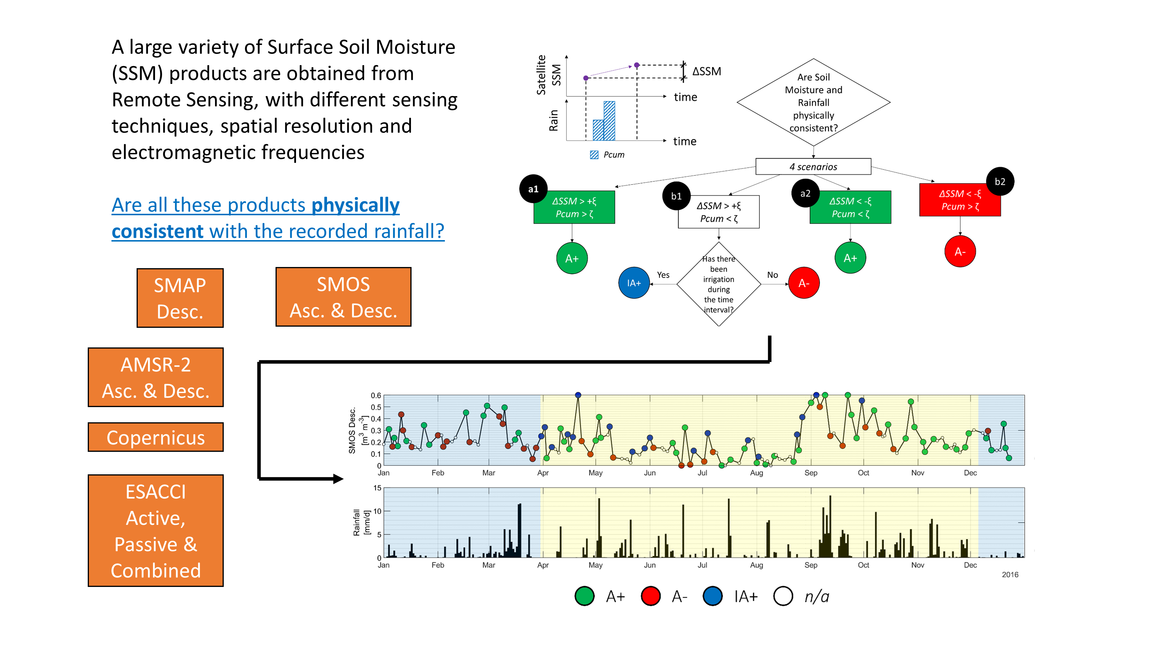
1. Introduction
- (i)
- Establish a methodology to measure the “physical” reliability/consistency of a given dataset
- (ii)
- Discern the differences between the various datasets and identify the possible background reasons
- (i)
- Data uncertainties are assumed to be stationary, although varying vegetation conditions can influence SSM retrieval over the course of different months;
- (ii)
- Merging algorithms, used to obtain long-spanning SSM records from different instruments, “give rise to unique error characteristics such as highly non-stationary errors due to the intermittent and weighted use of retrievals from different sensors or inhomogeneities between sensor transition periods”.
2. Materials and Methods
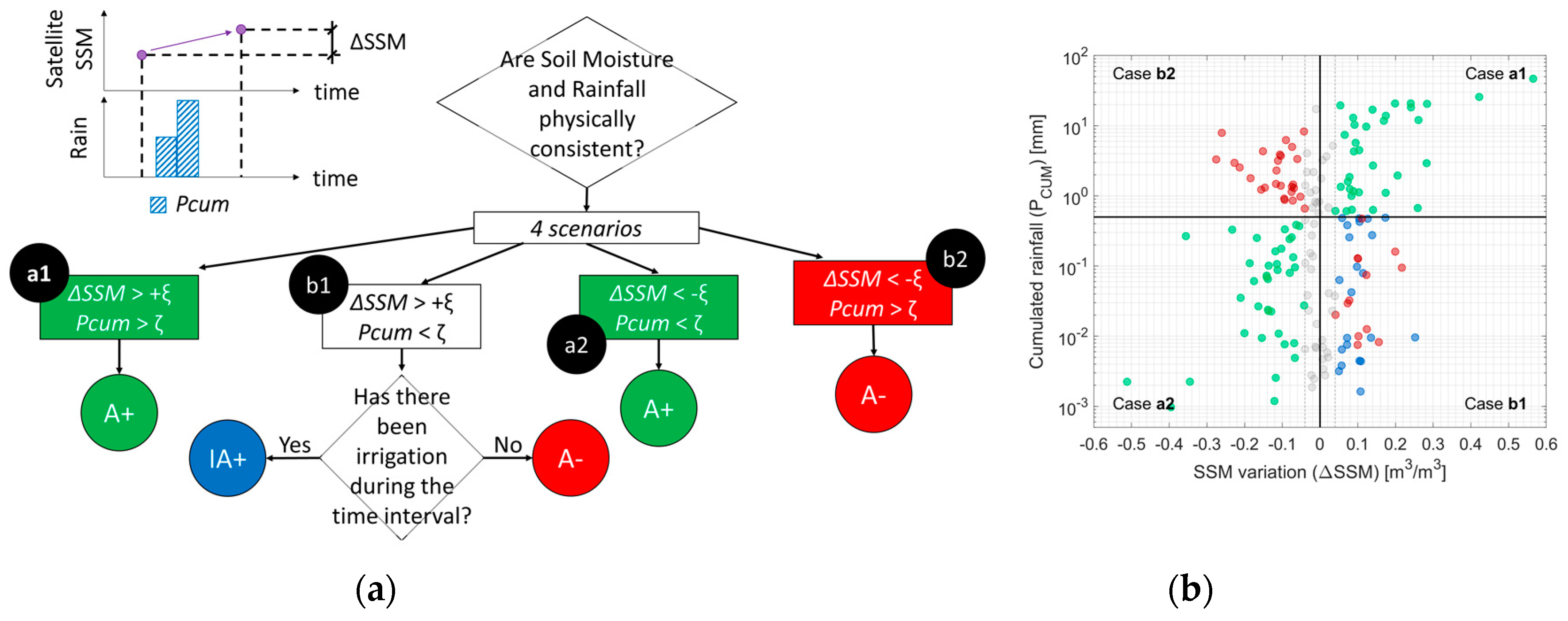
2.1. Hydrological Consistency Index (HCI) Methodology
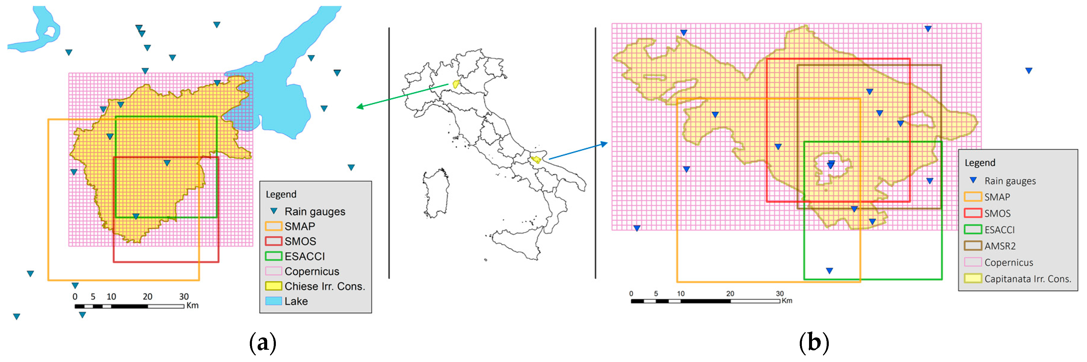
2.2. Case Studies
2.3. Remote Sensing Surface Soil Moisture Datasets
2.4. Precipitation Dataset
3. Results
3.1. Correlation between SSM and Precipitation
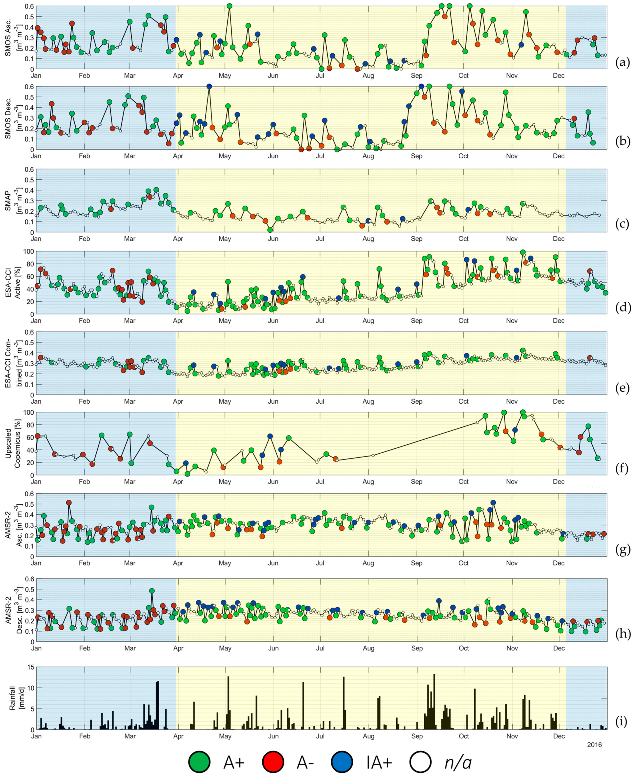
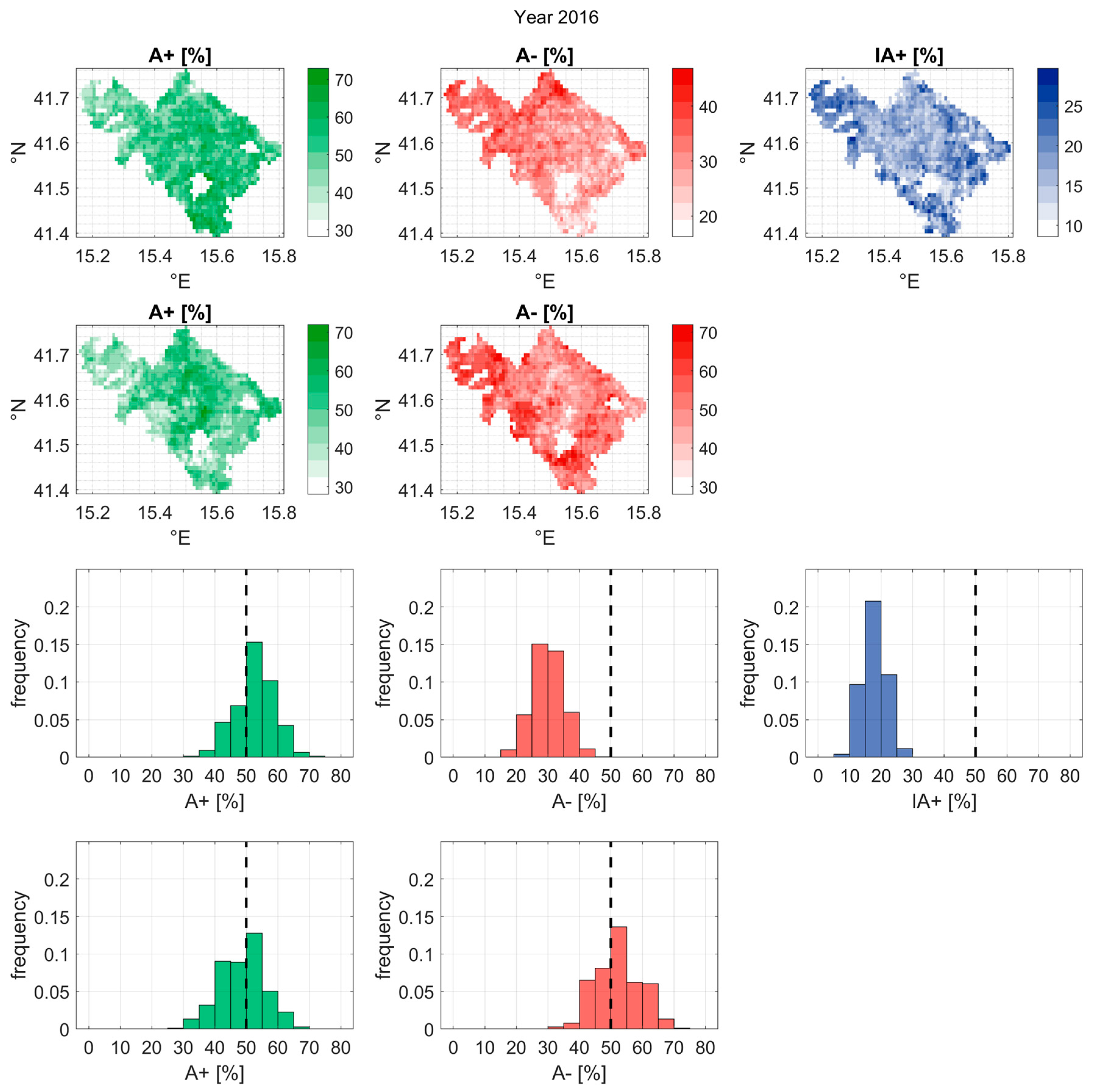
3.2. Consistency for Capitanata Irrigation Consortium
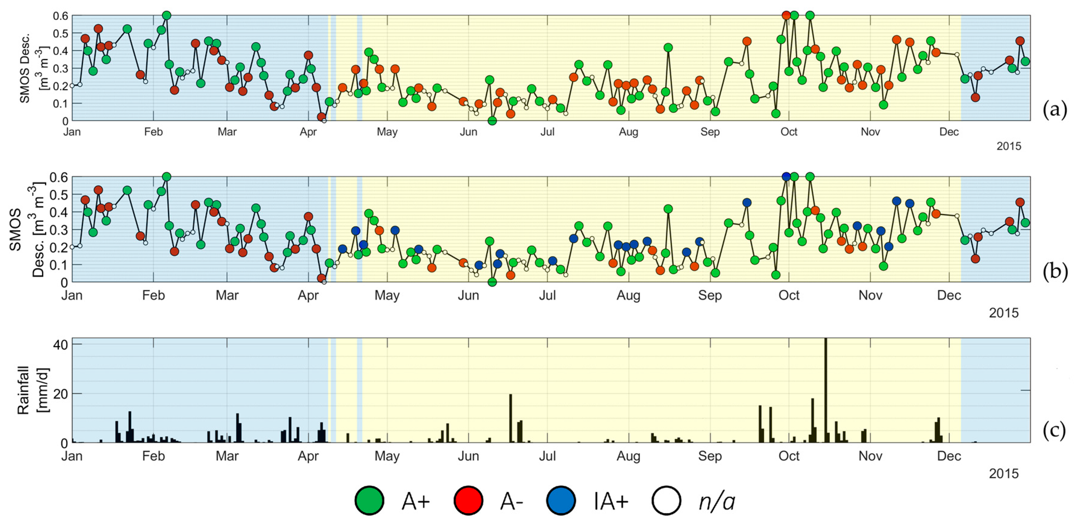
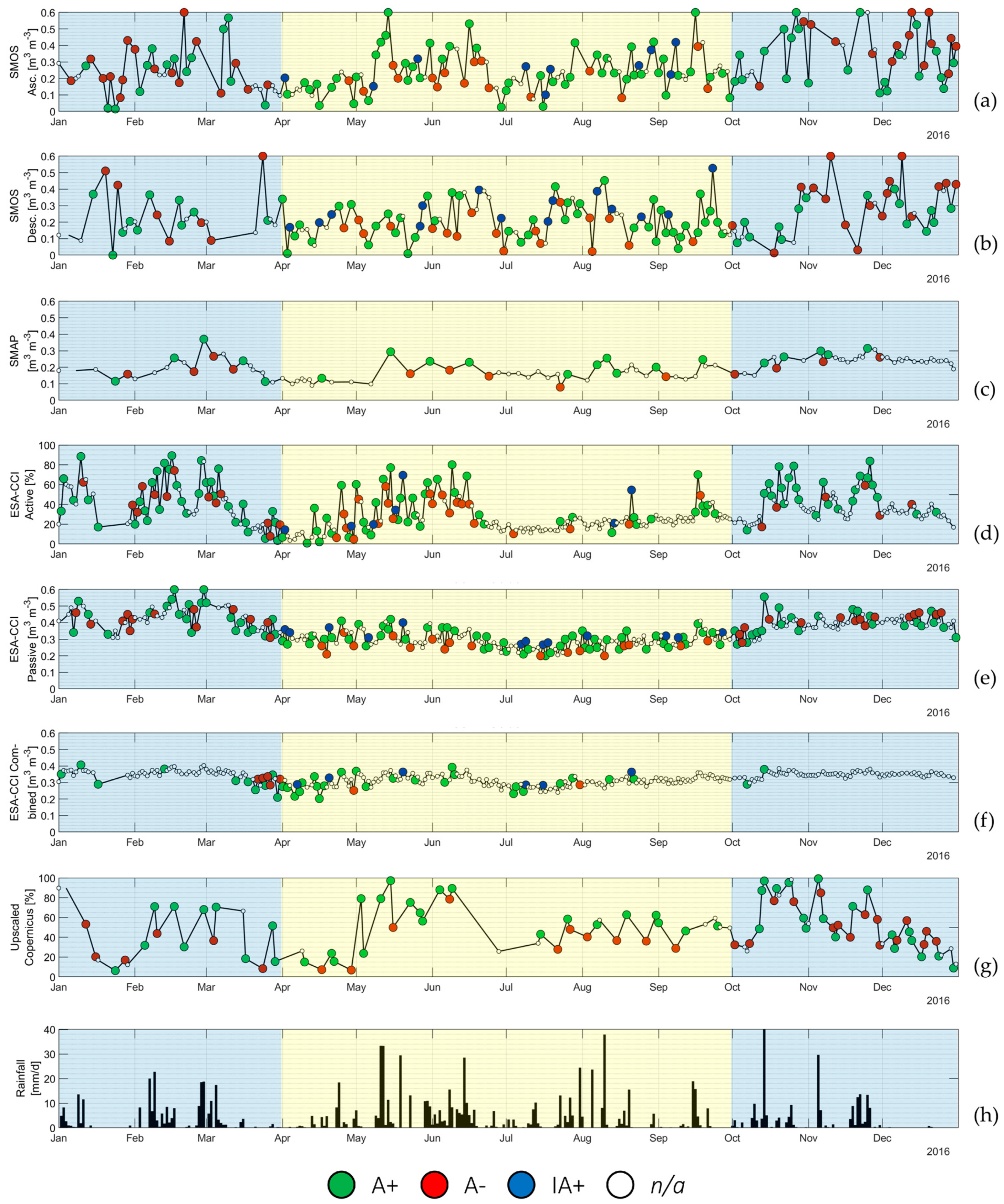
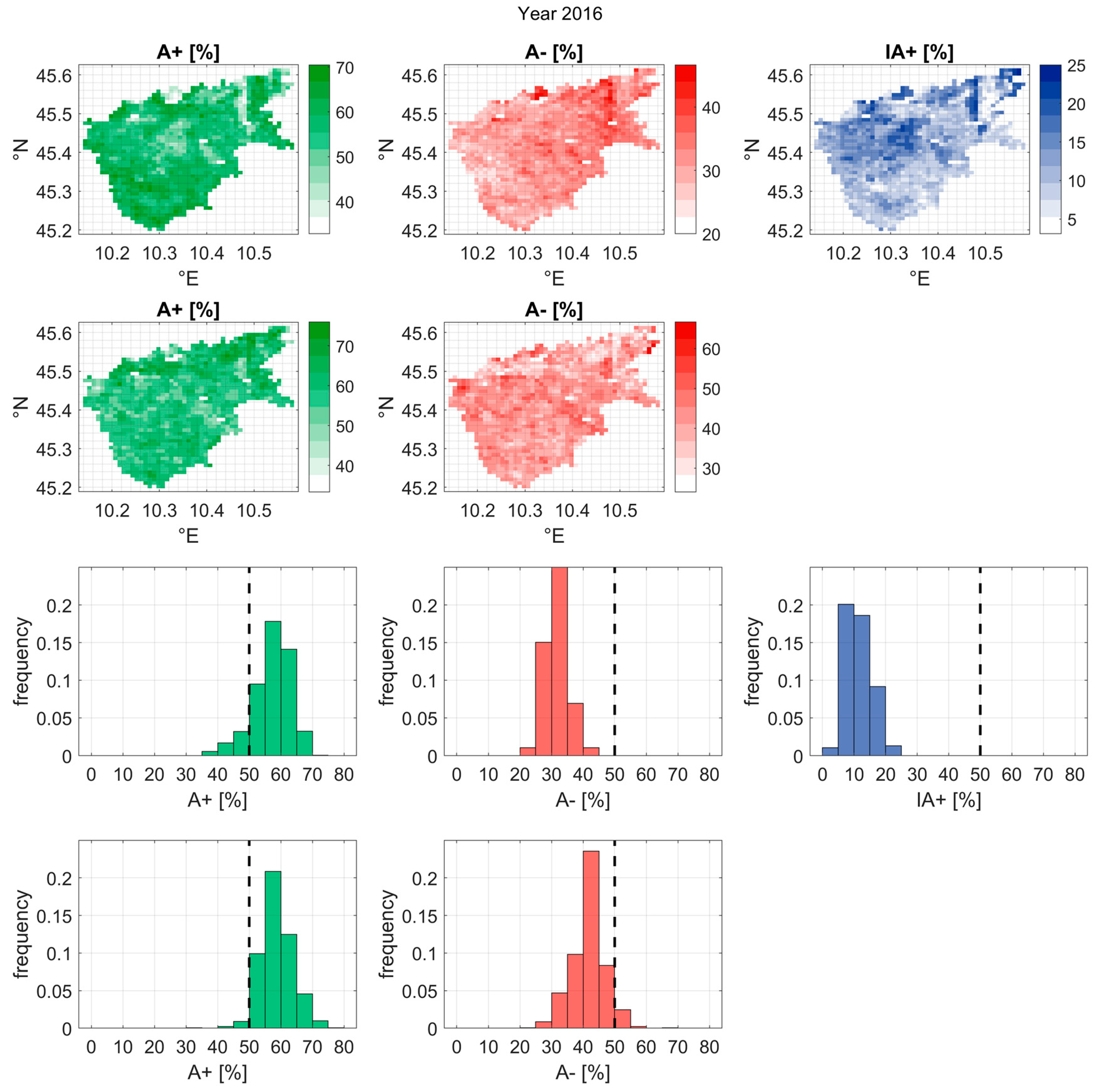
3.3. Consistency for Chiese Irrigation Consortium
3.4. Capitanata–Chiese Comparison
3.5. Retrieval Technology and Algorithm Comparison
3.6. Spatial Resolution Differences with Copernicus
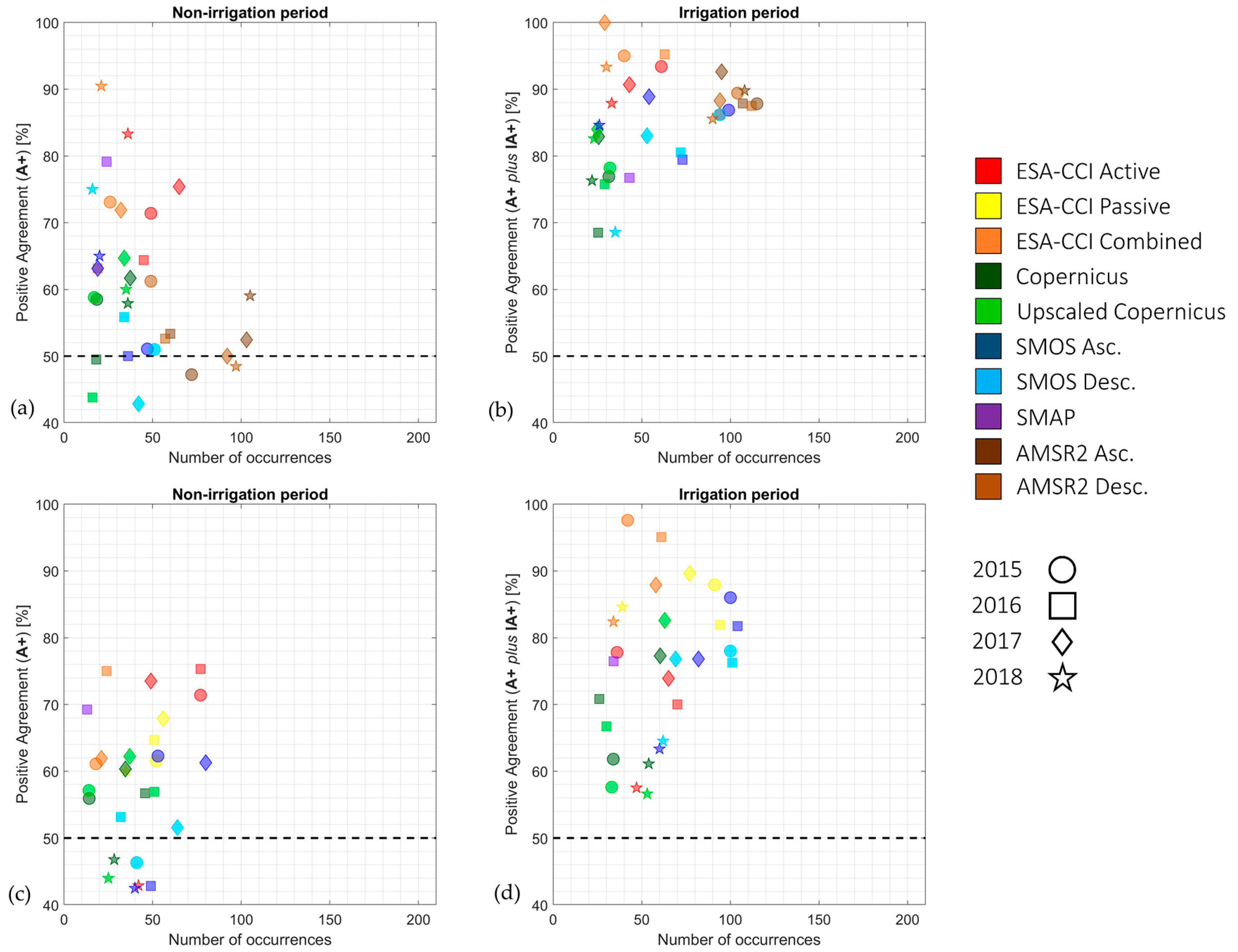
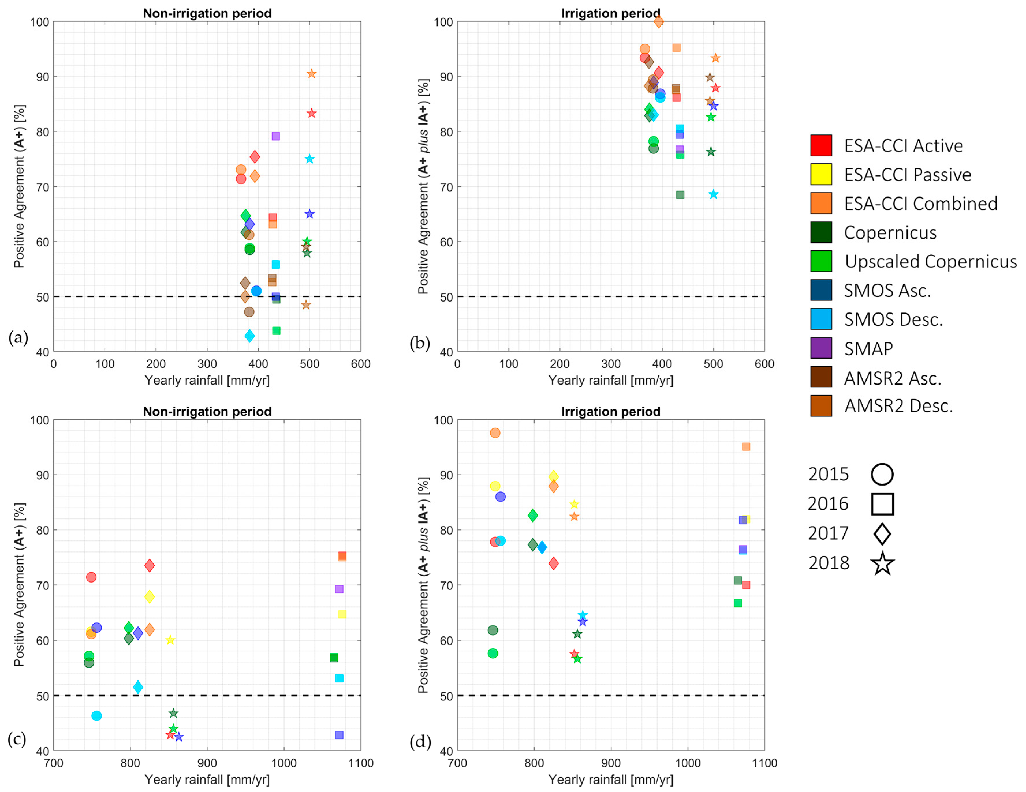
3.7. Incidence of Yearly Rainfall and Data Density
3.8. Hit Rate and False Positives Check
4. Discussion
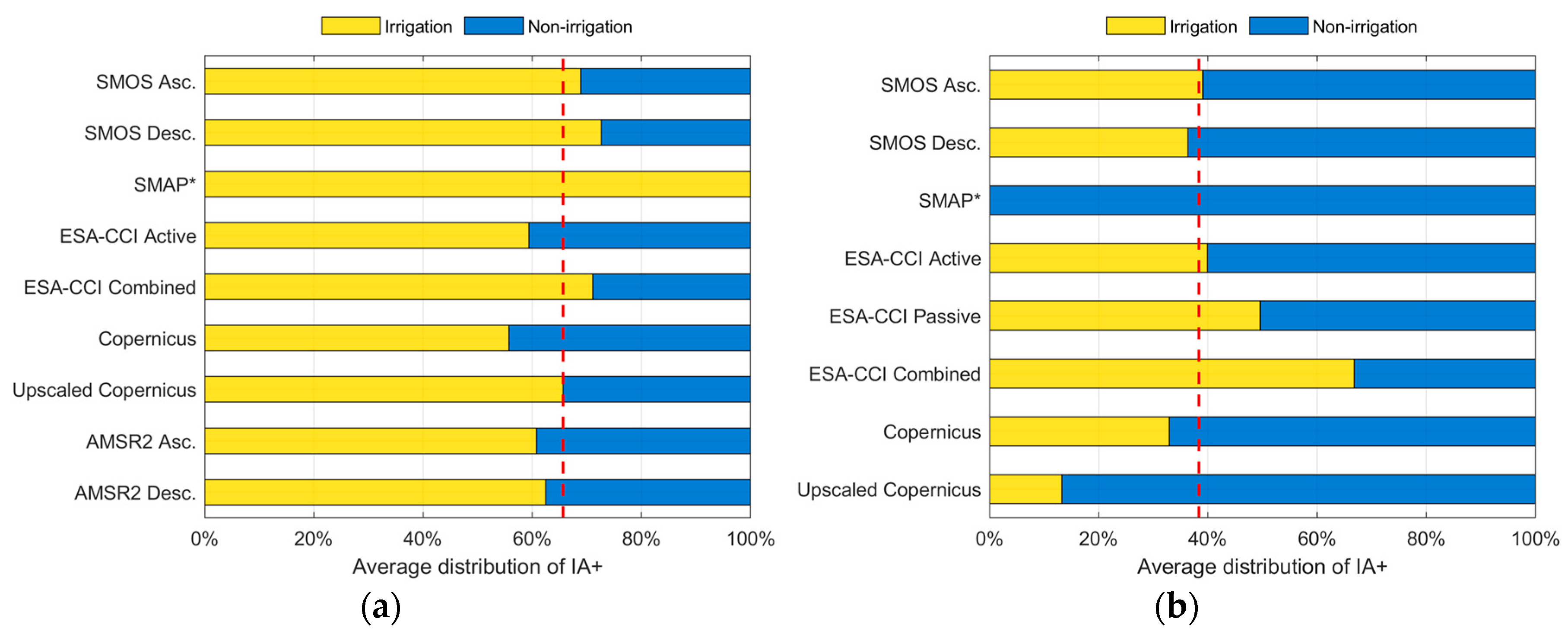
- By retrieval technology. Active and passive measurements have not shown major performance differences, while hybrid estimates (combination of both active and passive direct measurements) have displayed better performances, relying less on irrigation to achieve hydrological consistency (IA+ averaging 10% for hybrid, against 17% and 22% for active and passive, respectively).
- By spatial resolution. The Copernicus dataset is the only high-resolution dataset of the group (1 km), and it has been upscaled to a scale similar to the other datasets (30 km) in order to understand the influence of scale on its results. While no noticeable difference was found between the two versions of Copernicus SSM, the high-resolution dataset guaranteed a wide heterogeneity at local (crop field) level that could be interesting to analyze with high-resolution irrigation data.
- By test case wetness. Separating the results by yearly rainfall allowed us to understand if higher amounts of precipitation could hamper the accuracy of HCI by providing better results. No clear trends were found in this matter.
- By data density. Different datasets have different time frequencies, ranging from one estimate a day (ESA-CCI) up to one estimate every 4 days (Copernicus). These different densities could provide different relevance to some datasets over others. Actually, a higher result dispersion was found for datasets (and years) with less yearly SSM retrievals, with more compact values for higher data densities. However, no clear trend (e.g., better/worse results with less available data) was detected.
- (i)
- Information about irrigation may not be complete: unregistered irrigation volumes (e.g., those related to unrecorded private wells) can provide explanation for increasing SSM values in absence of precipitation even outside of the “official” irrigation season. The integration of this kind of data would have immediate effect in improving the HR seen in Section 3.8;
- (ii)
- The algorithm does not take into account daily evapotranspiration: especially in the warmer months of the year, sometimes, the actual evapotranspiration can be high enough that even though some rainfall has been registered, the overall water balance in the soil results negative, implying an SSM decrease;
- (iii)
- The presence of vegetation can alter the SSM retrieval process for non-L-band satellites: although no clear difference has emerged between L-band (i.e., SMOS and SMAP) and C-band (i.e., Copernicus and AMSR2) datasets, it is reasonable to assume that vegetation contributes to the hydrological inconsistencies found in our analysis. For example, the fact that the Chiese case is more vegetated than the Capitanata one may be part of the reason for a higher average inconsistency in Chiese (22%) than in Capitanata (15%).
5. Conclusions
Author Contributions
Funding
Conflicts of Interest
References
- Corbari, C.; Ravazzani, G.; Martinelli, J.; Mancini, M. Elevation based correction of snow coverage retrieved from satellite images tom improve model calibration. Hydrol. Earth Syst. Sci. 2009, 13, 639–649. [Google Scholar] [CrossRef]
- Su, Z. The Surface Energy Balance System (SEBS) for estimation of turbulent heat fluxes. Hydrol. Earth Syst. Sci. 2002, 6, 85–99. [Google Scholar] [CrossRef]
- Corbari, C.; Mancini, M. Calibration and Validation of a Distributed Energy-Water Balance Model Using Satellite Data of Land Surface Temperature and Ground Discharge Measurements. J. Hydrometeorol. 2014, 15, 376–392. [Google Scholar] [CrossRef]
- Xu, W.; Ren, X.; Smith, A. Remote Sensing, Crop Yield Estimation and Agricultural Vulnerability Assessment: A Case of Southern Alberta. In Proceedings of the 19th International Conference on Geoinformatics, Shanghai, China, 24–26 June 2011; pp. 1–7. [Google Scholar] [CrossRef]
- Tarpanelli, A.; Brocca, L.; Lacava, T.; Faruolo, M.; Melone, F.; Moramarco, T.; Pergola, N.; Tramutoli, V. River discharge estimation through MODIS data. SPIE Remote Sens. 2011, 8174, 817408. [Google Scholar] [CrossRef]
- Joshi, N.; Baumann, M.; Ehammer, A.; Fensholt, R.; Grogan, K.; Hostert, P.; Jepsen, M.R.; Kuemmerle, T.; Meyfroidt, P.; Mitchard, E.T.A.; et al. A Review of the Application of Optical and Radar Remote Sensing Data Fusion to Land Use Mapping and Monitoring. Remote Sens. 2016, 8, 70. [Google Scholar] [CrossRef]
- Dorigo, W.; Oevelen, P.; Wagner, W.; Drusch, M.; Mecklenburg, S.; Robock, A.; Jackson, T. A New International Network for in Situ Soil Moisture Data. Eos Trans. 2011, 92, 141–142. [Google Scholar] [CrossRef]
- Piles, M.; Sanchez, N.; Vall-Llossera, M.; Camps, A.; Martinez-Fernandez, J.; Martinez, J.; Gonzalez-Gambau, V. A Downscaling Approach for SMOS Land Observations: Evaluation of High-Resolution Soil Moisture Maps Over the Iberian Peninsula. IEEE J. Sel. Top. Appl. Earth Obs. Remote Sens. 2014, 7, 3845–3857. [Google Scholar] [CrossRef]
- Grayson, R.; Blöschl, G. Spatial Patterns in Catchment Hydrology: Observations and Modelling; Cambridge University Press: Cambridge, UK, 2000. [Google Scholar]
- Ochsner, T.E.; Cosh, M.H.; Cuenca, R.H.; Dorigo, W.A.; Draper, C.S.; Hagimoto, Y.; Kerr, Y.H.; Larson, K.M.; Njoku, E.G.; Small, E.E.; et al. State of the Art in Large-Scale Soil Moisture Monitoring. Soil Sci. Soc. Am. J. 2013, 77, 1888–1919. [Google Scholar] [CrossRef]
- Molero, B.; Leroux, D.J.; Richaume, P.; Kerr, Y.H.; Merlin, O.; Cosh, M.; Bindlish, R. Multi-Timescale Analysis of the Spatial Representativeness of In Situ Soil Moisture Data within Satellite Footprints. J. Geophys. Res. Atmos. 2018, 123, 3–21. [Google Scholar] [CrossRef] [PubMed]
- Mohanty, B.P.; Cosh, M.H.; Lakshmi, V.; Montzka, C. Soil Moisture Remote Sensing: State-of-the-Science. Vadose Zone J. 2017, 16, 1–9. [Google Scholar] [CrossRef]
- Das, K.; Paul, P.K. Present status of soil moisture estimation by microwave remote sensing. Cogent Geosci. 2015, 1. [Google Scholar] [CrossRef]
- Nichols, S.; Zhang, Y.; Ahmad, A. Review and evaluation of remote sensing methods for soil-moisture estimation. J. Photon. Energy 2011, 2, 28001. [Google Scholar] [CrossRef]
- Paloscia, S. Remote Sensing of Soil Moisture. In Radiation and Water in the Climate System; Raschke, E., Ed.; Springer: Berlin/Heidelberg, Germany, 1996; Volume 45. [Google Scholar] [CrossRef]
- Njoku, E.G.; Entekhabi, D. Passive microwave remote sensing of soil moisture. J. Hydrol. 1996, 184, 101–129. [Google Scholar] [CrossRef]
- Kerr, Y.H.; Waldteufel, P.; Richaume, P.; Wigneron, J.P.; Ferrazzoli, P.; Mahmoodi, A.; Al Bitar, A.; Cabot, F.; Gruhier, C.; Juglea, S.E.; et al. The SMOS Soil Moisture Retrieval Algorithm. IEEE Trans. Geosci. Remote Sens. 2012, 50, 1384–1403. [Google Scholar] [CrossRef]
- Fernandez-Moran, R.; Wigneron, J.P.; De Lannoy, G.; Lopez-Baeza, E.; Parrens, M.; Mialon, A.; Mahmoodi, A.; Al-Yaari, A.; Bircher, S.; Al Bitar, A.; et al. A new calibration of the effective scattering albedo and soil roughness parameters in the SMOS SM retrieval algorithm. Int. J. Appl. Earth Obs. Geoinf. 2017, 62, 27–38. [Google Scholar] [CrossRef]
- Tomer, S.K.; Al Bitar, A.; Sekhar, M.; Zribi, M.; Bandyopadhyay, S.; Kerr, Y.H. MAPSM: A Spatio-Temporal Algorithm for Merging Soil Moisture from Active and Passive Microwave Remote Sensing. Remote Sens. 2016, 8, 990. [Google Scholar] [CrossRef]
- Malbéteau, Y.; Merlin, O.; Balsamo, G.; Er-Raki, S.; Khabba, S.; Walker, J.P.; Jarlan, L. Toward a Surface Soil Moisture Product at High Spatiotemporal Resolution: Temporally Interpolated, Spatially Disaggregated SMOS Data. J. Hydrometeorol. 2018, 19, 183–200. [Google Scholar] [CrossRef]
- Justice, C.; Belward, A.; Morisette, J.; Lewis, P.; Privette, J.; Baret, F. Developments in the ’validation’ of satellite sensor products for the study of the land surface. Int. J. Remote Sens. 2000, 21, 3383–3390. [Google Scholar] [CrossRef]
- Jackson, T.J.; Cosh, M.H.; Bindlish, R.; Starks, P.J.; Bosch, D.D.; Seyfried, M.; Goodrich, D.; Moran, M.S.; Du, J. Validation of Advanced Microwave Scanning Radiometer Soil Moisture Products. IEEE Trans. Geosci. Remote Sens. 2010, 48, 4256–4272. [Google Scholar] [CrossRef]
- Colliander, A.; Jackson, T.J.; Bindlish, R.; Chan, S.; Das, N.; Kim, S.B.; Cosh, M.H.; Dunbar, R.S.; Dang, L.; Pashaian, L.; et al. Validation of SMAP surface soil moisture products with core validation sites. Remote Sens. Environ. 2017, 191, 215–231. [Google Scholar] [CrossRef]
- Brocca, L.; Hasenauer, S.; Lacava, T.; Melone, F.; Moramarco, T.E.; Wagner, W.; Dorigo, W.; Matgen, P.; Martínez-Fernández, J.; Llorens, P.; et al. Soil moisture estimation through ASCAT and AMSR-E sensors: An intercomparison and validation study across Europe. Remote Sens. Environ. 2011, 115, 3390–3408. [Google Scholar] [CrossRef]
- Al Bitar, A.; Leroux, D.J.; Kerr, Y.H.; Merlin, O.; Richaume, P.; Sahoo, A.; Wood, E.F. Evaluation of SMOS Soil Moisture Products Over Continental, U.S. Using the SCAN/SNOTEL Network. IEEE Trans. Geosci. Remote Sens. 2012, 50, 1572–1586. [Google Scholar] [CrossRef]
- Kerr, Y.H.; Al-Yaari, A.; Rodriguez-Fernandez, N.; Parrens, M.; Molero, B.; Leroux, D.; Bircher, S.; Mahmoodi, A.; Mialon, A.; Richaume, P.; et al. Overview of SMOS performance in terms of global soil moisture monitoring after six years in operation. Remote Sens. Environ. 2016, 180, 40–63. [Google Scholar] [CrossRef]
- Cui, C.; Xu, J.; Zeng, J.; Chen, K.-S.; Bai, X.; Lu, H.; Chen, Q.; Zhao, T. Soil Moisture Mapping from Satellites: An Intercomparison of SMAP, SMOS, FY3B, AMSR2, and ESA CCI over Two Dense Network Regions at Different Spatial Scales. Remote Sens. 2017, 10, 33. [Google Scholar] [CrossRef]
- El Hajj, M.; Baghdadi, N.; Zribi, M.; Rodríguez-Fernández, N.J.; Wigneron, J.-P.; Al-Yaari, A.; Al Bitar, A.; Albergelb, C.; Albergel, C. Evaluation of SMOS, SMAP, ASCAT and Sentinel-1 Soil Moisture Products at Sites in Southwestern France. Remote Sens. 2018, 10, 569. [Google Scholar] [CrossRef]
- Chen, F.; Crow, W.T.; Bindlish, R.; Colliander, A.; Burgin, M.S.; Asanuma, J.; Aida, K. Global-scale evaluation of SMAP, SMOS and ASCAT soil moisture products using triple collocation. Remote Sens. Environ. 2018, 214, 1–13. [Google Scholar] [CrossRef]
- Gruber, A.; Su, C.-H.; Zwieback, S.; Crow, W.; Dorigo, W.; Wagner, W. Recent advances in (soil moisture) triple collocation analysis. Int. J. Appl. Earth Obs. Geoinf. 2016, 45, 200–211. [Google Scholar] [CrossRef]
- Meingast, K.M.; Falkowski, M.J.; Kane, E.S.; Potvin, L.R.; Benscoter, B.W.; Smith, A.M.; Bourgeau-Chavez, L.; Miller, M.E. Spectral detection of near-surface moisture content and water-table position in northern peatland ecosystems. Remote Sens. Environ. 2014, 152, 536–546. [Google Scholar] [CrossRef]
- Brocca, L.; Tarpanelli, A.; Filippucci, P.; Dorigo, W.; Zaussinger, F.; Gruber, A.; Fernández-Prieto, D. How much water is used for irrigation? A new approach exploiting coarse resolution satellite soil moisture products. Int. J. Appl. Earth Obs. Geoinf. 2018, 73, 752–766. [Google Scholar] [CrossRef]
- Lawston, P.M.; Santanello, J.A.; Kumar, S.V. Irrigation Signals Detected From SMAP Soil Moisture Retrievals. Geophys. Res. Lett. 2017, 44, 11860–11867. [Google Scholar] [CrossRef]
- Zhang, X.; Qiu, J.; Leng, G.; Yang, Y.; Gao, Q.; Fan, Y.; Luo, J. The Potential Utility of Satellite Soil Moisture Retrievals for Detecting Irrigation Patterns in China. Water 2018, 10, 1505. [Google Scholar] [CrossRef]
- Zaussinger, F.; Dorigo, W.; Gruber, A.; Tarpanelli, A.; Filippucci, P.; Brocca, L. Estimating irrigation water use over the contiguous United States by combining satellite and reanalysis soil moisture data. Hydrol. Earth Syst. Sci. 2019, 23, 897–923. [Google Scholar] [CrossRef]
- Dai, A.; Trenberth, K.E.; Karl, T.R. Effects of Clouds, Soil Moisture, Precipitation, and Water Vapour on Diurnal Temperature Range. J. Clim. 1999, 12, 2451–2473. [Google Scholar] [CrossRef]
- Sehler, R.; Li, J.; Reager, J.T.; Ye, H. Investigating Relationship Between Soil Moisture and Precipitation Globally Using Remote Sensing Observations. J. Contemp. Water Res. Educ. 2019, 168, 106–118. [Google Scholar] [CrossRef]
- McCabe, M.F.; Wood, E.; Wójcik, R.; Pan, M.; Sheffield, J.; Gao, H.; Su, H. Hydrological consistency using multi-sensor remote sensing data for water and energy cycle studies. Remote Sens. Environ. 2008, 112, 430–444. [Google Scholar] [CrossRef]
- Meng, X.; Li, R.; Luan, L.; Lyu, S.; Zhang, T.; Ao, Y.; Han, B.; Zhao, L.; Ma, Y. Detecting hydrological consistency between soil moisture and precipitation and changes of soil moisture in summer over the Tibetan Plateau. Clim. Dyn. 2017, 51, 4157–4168. [Google Scholar] [CrossRef]
- Gruber, A.; De Lannoy, G.; Albergel, C.; Al-Yaari, A.; Brocca, L.; Calvet, J.-C.; Colliander, A.; Cosh, M.; Crow, W.; Dorigo, W.; et al. Validation practices for satellite soil moisture retrievals: What are (the) errors? Remote Sens. Environ. 2020, 244, 111806. [Google Scholar] [CrossRef]
- Agenzia Regionale per la Prevenzione e la Protezione dell’Ambiente (ARPA) Puglia. Available online: http://www.arpa.puglia.it/web/guest/serviziometeo (accessed on 7 August 2020).
- Kerr, Y.H.; Waldteufel, P.; Wigneron, J.-P.; Delwart, S.; Cabot, F.; Boutin, J.; Escorihuela, M.-J.; Font, J.; Reul, N.; Gruhier, C.; et al. The SMOS Mission: New Tool for Monitoring Key Elements ofthe Global Water Cycle. Proc. IEEE 2010, 98, 666–687. [Google Scholar] [CrossRef]
- Ulaby, F.T.; Moore, M.K.; Fung, A.K. Microwave Remote Sensing, Active and Passive; Artech House: Norwood, MA, USA, 1982; Volume 2. [Google Scholar]
- SMOS Level 2 Processor Soil Moisture ATBD from ESA Earth Online. Available online: https://earth.esa.int/documents/10174/1854519/SMOS_L2_SM_ATBD (accessed on 7 August 2020).
- Al Bitar, A.; Mialon, A.; Kerr, Y.H.; Cabot, F.; Richaume, P.; Jacquette, E.; Quesney, A.; Mahmoodi, A.; Tarot, S.; Parrens, M.; et al. The global SMOS Level 3 daily soil moisture and brightness temperature maps. Earth Syst. Sci. Data 2017, 9, 293–315. [Google Scholar] [CrossRef]
- Entekhabi, D.; Yueh, S.; O’Neill, P.E.; Kellogg, K.H.; Allen, A.; Bindlish, R.; Johnson, J. SMAP Handbook—Soil Moisture Active Passive—Mapping Soil Moisture and Freeze/Thaw from Space; Laboratory, J.P., Ed.; JPL Publication: Pasadena, CA, USA, 2014; pp. 400–1567. [Google Scholar]
- Gruber, A.; Scanlon, T.; Van Der Schalie, R.; Wagner, W.; Dorigo, W. Evolution of the ESA CCI Soil Moisture climate data records and their underlying merging methodology. Earth Syst. Sci. Data 2019, 11, 717–739. [Google Scholar] [CrossRef]
- Naeimi, V.; Scipal, K.; Bartalis, Z.; Hasenauer, S.; Wagner, W. An Improved Soil Moisture Retrieval Algorithm for ERS and METOP Scatterometer Observations. IEEE Trans. Geosci. Remote Sens. 2009, 47, 1999–2013. [Google Scholar] [CrossRef]
- Liu, Y.; Dorigo, W.; Parinussa, R.; De Jeu, R.; Wagner, W.; McCabe, M.F.; Evans, J.; Van Dijk, A. Trend-preserving blending of passive and active microwave soil moisture retrievals. Remote Sens. Environ. 2012, 123, 280–297. [Google Scholar] [CrossRef]
- Gruber, A.; Dorigo, W.; Crow, W.; Wagner, W. Triple Collocation-Based Merging of Satellite Soil Moisture Retrievals. IEEE Trans. Geosci. Remote Sens. 2017, 55, 6780–6792. [Google Scholar] [CrossRef]
- Dorigo, W.; Wagner, W.; Albergel, C.; Albrecht, F.; Balsamo, G.; Brocca, L.; Chung, D.; Ertl, M.; Forkel, M.; Gruber, A.; et al. ESA CCI Soil Moisture for improved Earth system understanding: State-of-the art and future directions. Remote Sens. Environ. 2017, 203, 185–215. [Google Scholar] [CrossRef]
- Bauer-Marschallinger, B.; Paulik, C.; Hochstöger, S.; Mistelbauer, T.; Modanesi, S.; Ciabatta, L.; Massari, C.; Brocca, L.; Wagner, W. Soil Moisture from Fusion of Scatterometer and SAR: Closing the Scale Gap with Temporal Filtering. Remote Sens. 2018, 10, 1030. [Google Scholar] [CrossRef]
- de Jeu, R.; Owe, M. AMSR2/GCOM-W1 Surface Soil Moisture (LPRM) L3 1 Day 10 km × 10 km Descending V001; Bill, T., Ed.; Goddard Earth Sciences Data and Information Services Center (GES DISC): Greenbelt, MD, USA, 2014. [Google Scholar] [CrossRef]
- Scanlon, T.; Dorigo, W.; Preimesberger, W.; Kidd, R.; van der Schalie, R.; de Jeu, R.; Thevenon, H. Algorithm Development Plan (ADP)—D1.2 Version 0.1. 2019, deliverable D1.2 ADP for the ESA Climate Change Initiative Plus Soil Moisture Project (ESRIN Contract no: 4000126684/19/I-NB). Available online: https://www.esa-soilmoisture-cci.org/sites/default/files/documents/ESA_CCI_SM_ADP_version_1.0.pdf (accessed on 10 November 2020).
- Bauer-Marschallinger, B.; Paulik, C. Product user manual—Surface Soil Moisture—Collection 1 km—Version 1. 2019 Copernicus Land Operations “Vegetation and Energy”, Date Issued: 08/04/2020. Available online: https://land.copernicus.eu/global/sites/cgls.vito.be/files/products/CGLOPS1_PUM_SWI1km-V1_I1.20.pdf (accessed on 10 November 2020).
- Njoku, E.G.; Chan, S.K. Vegetation and surface roughness effects on AMSR-E land observations. Remote Sens. Environ. 2006, 100, 190–199. [Google Scholar] [CrossRef]
- Qiu, J.; Crow, W.T.; Wagner, W.; Zhao, T. Effect of vegetation index choice on soil moisture retrievals via the synergistic use of synthetic aperture radar and optical remote sensing. Int. J. Appl. Earth Obs. Geoinf. 2019, 80, 47–57. [Google Scholar] [CrossRef]


| Dataset | Product | Ref. Time | Retrieval Technology | E.M. Spectrum | Revisit Time | Sensor Grid | Product Grid | Source |
|---|---|---|---|---|---|---|---|---|
| SMOS | Ascending Descending | 06:00 18:00 | Passive | L band | 1-2 days | 40 km | 25 km | [44] |
| SMAP | Descending | 18:00 | Passive | L band | 2.2 days | 40 km | 36 km | [46] |
| ESA-CCI | Active Passive Combined | 00:00 | Active Passive Hybrid | Various bands | 1.2 days | Variable | 0.25° | [47] |
| Copernicus (Sentinel1) | Original Upscaled | 00:00 | Active | C band | 4.1 days | 10 m | 1°/112 30 km | [52] |
| AMSR-2 | Ascending Descending | 13:00 01:00 | Passive | C band | 1.5 days | 50 × 70 m | 10 km | [53] |
| Dataset | Capitanata | Chiese | ||
|---|---|---|---|---|
| Pearson | Spearman | Pearson | Spearman | |
| ESA-CCI Active | 0.1644 | 0.2775 | 0.2120 | 0.3039 |
| ESA-CCI Passive | --- | --- | 0.0846 | 0.1076 |
| ESA-CCI Combined | 0.1312 | 0.3080 | 0.1056 | 0.2053 |
| Copernicus | 0.3806 | 0.4174 | 0.2977 | 0.3035 |
| Copernicus Upscaled | 0.4173 | 0.4499 | 0.3406 | 0.3629 |
| SMOS Asc. | 0.2396 | 0.2928 | 0.1192 | 0.1451 |
| SMOS Desc. | 0.0381 | 0.0667 | 0.0552 | 0.0918 |
| SMAP | 0.3929 | 0.4270 | 0.1770 | 0.2494 |
| AMSR-2 Asc. | 0.1189 | 0.1203 | --- | --- |
| AMSR-2 Desc. | 0.1016 | 0.1224 | --- | --- |
| Irrigation Regime | Simple HCI (No Irrigation) | Complete HCI (With Irrigation) | ||
|---|---|---|---|---|
| Non-Irrigation period | A+ | 26 (51%) | A+ | 26 (51%) |
| A− | 25 (49%) | A− | 25 (49%) | |
| Irrigation period | A+ | 57 (61%) | A+ | 57 (61%) |
| A− | 37 (29%) | A− | 13 (14%) | |
| IA+ | 24 (26%) | |||
| Dataset | 2015 | 2016 | 2017 | 2018 | ||||||||
|---|---|---|---|---|---|---|---|---|---|---|---|---|
| n | A+ | A− | n | A+ | A− | n | A+ | A− | n | A+ | A− | |
| Active | 49 | 71% | 29% | 45 | 64% | 36% | 65 | 75% | 25% | 36 | 83% | 17% |
| Combined | 26 | 69% | 31% | 19 | 58% | 42% | 32 | 72% | 28% | 21 | 90% | 10% |
| Copernicus | 18.5 | 59% | 41% | 18.1 | 50% | 50% | 37.3 | 62% | 38% | 36.0 | 58% | 42% |
| Up. Copernicus | 17 | 59% | 41% | 16 | 44% | 56% | 34 | 65% | 35% | 35 | 60% | 40% |
| SMOS Asc. | 46 | 50% | 50% | 36 | 50% | 50% | 19 | 63% | 37% | 22 | 68% | 32% |
| SMOS Desc. | 50 | 50% | 50% | 34 | 56% | 44% | 41 | 44% | 56% | 16 | 75% | 25% |
| SMAP | - | - | - | 24 | 79% | 21% | - | - | - | - | - | - |
| AMSR2 Asc. | 48 | 60% | 40% | 57 | 53% | 47% | 92 | 50% | 50% | 97 | 48% | 52% |
| AMSR2 Desc. | 71 | 48% | 52% | 60 | 53% | 47% | 103 | 52% | 48% | 105 | 59% | 41% |
| Dataset | 2015 | 2016 | 2017 | 2018 | ||||||||||||
|---|---|---|---|---|---|---|---|---|---|---|---|---|---|---|---|---|
| n | A+ | A− | IA+ | n | A+ | A− | IA+ | n | A+ | A− | IA+ | n | A+ | A− | IA+ | |
| Active | 61 | 75% | 7% | 18% | 94 | 70% | 14% | 16% | 43 | 70% | 9% | 21% | 33 | 67% | 12% | 21% |
| Combined | 40 | 65% | 8% | 28% | 63 | 71% | 10% | 19% | 29 | 76% | -% | 24% | 30 | 63% | 13% | 23% |
| Copernicus | 31.4 | 65% | 23% | 12% | 25 | 51% | 31% | 18% | 26 | 62% | 17% | 21% | 22 | 63% | 23% | 14% |
| Up. Copernicus | 32 | 69% | 22% | 9% | 29 | 59% | 24% | 17% | 25 | 60% | 16% | 24% | 23 | 74% | 17% | 9% |
| SMOS Asc. | 102 | 56% | 16% | 28% | 76 | 61% | 22% | 17% | 58 | 71% | 10% | 19% | 26 | 62% | 15% | 23% |
| SMOS Desc. | 95 | 59% | 16% | 25% | 72 | 49% | 25% | 26% | 53 | 53% | 19% | 28% | 35 | 31% | 31% | 37% |
| SMAP | ₋ | ₋ | ₋ | ₋ | 44 | 64% | 30% | 7% | ₋ | ₋ | - | ₋ | ₋ | ₋ | ₋ | ₋ |
| AMSR2 Asc. | 105 | 55% | 13% | 31% | 112 | 46% | 22% | 31% | 94 | 54% | 13% | 33% | 90 | 49% | 17% | 34% |
| AMSR2 Desc. | 116 | 55% | 16% | 29% | 107 | 56% | 19% | 25% | 95 | 59% | 12% | 29% | 108 | 57% | 12% | 31% |
| Dataset | 2015 | 2016 | 2017 | 2018 | ||||||||
|---|---|---|---|---|---|---|---|---|---|---|---|---|
| n | A+ | A− | n | A+ | A− | n | A+ | A− | n | A+ | A− | |
| Active | 77 | 71% | 29% | 77 | 75% | 25% | 49 | 74% | 27% | 42 | 43% | 57% |
| Passive | 52 | 62% | 39% | 51 | 65% | 35% | 56 | 68% | 32% | 35 | 60% | 40% |
| Combined | 18 | 61% | 39% | 24 | 75% | 25% | 21 | 62% | 38% | 6 | 33% | 67% |
| Copernicus | 14.2 | 56% | 44% | 45.8 | 57% | 43% | 34.7 | 60% | 40% | 28.3 | 47% | 53% |
| Up. Copernicus | 14 | 57% | 43% | 51 | 57% | 43% | 37 | 62% | 38% | 25 | 44% | 56% |
| SMOS Asc. | 53 | 62% | 38% | 49 | 43% | 57% | 80 | 61% | 39% | 40 | 43% | 57% |
| SMOS Desc. | 41 | 46% | 54% | 32 | 53% | 47% | 64 | 52% | 48% | 39 | 36% | 64% |
| SMAP | - | - | - | 13 | 69% | 31% | - | - | - | - | - | - |
| Dataset. | 2015 | 2016 | 2017 | 2018 | ||||||||||||
|---|---|---|---|---|---|---|---|---|---|---|---|---|---|---|---|---|
| n | A+ | A− | IA+ | n | A+ | A− | IA+ | n | A+ | A− | IA+ | n | A+ | A− | IA+ | |
| Active | 36 | 67% | 22% | 11% | 70 | 60% | 30% | 10% | 65 | 59% | 26% | 15% | 47 | 51% | 43% | 6% |
| Passive | 91 | 74% | 12% | 14% | 94 | 70% | 18% | 12% | 77 | 75% | 10% | 14% | 39 | 72% | 15% | 13% |
| Combined | 42 | 84% | 2% | 14% | 61 | 84% | 5% | 11% | 58 | 79% | 12% | 9% | 34 | 77% | 18% | 5% |
| Copernicus | 33.9 | 57% | 38% | 5% | 26.0 | 64% | 29% | 7% | 60.3 | 70% | 23% | 7% | 53.9 | 57% | 39% | 4% |
| Up. Copernicus | 33 | 58% | 42% | -% | 30 | 67% | 33% | -% | 63 | 78% | 17% | 5% | 53 | 55% | 43% | 2% |
| SMOS Asc. | 100 | 65% | 14% | 21% | 104 | 66% | 18% | 16% | 82 | 56% | 23% | 21% | 60 | 50% | 37% | 13% |
| SMOS Desc. | 100 | 62% | 22% | 16% | 101 | 55% | 24% | 21% | 69 | 61% | 23% | 16% | 62 | 58% | 36% | 6% |
| SMAP | - | - | - | - | 34 | 77% | 23% | -% | - | - | - | - | - | - | - | - |
| Dataset | Capitanata | Chiese | ||||||||
|---|---|---|---|---|---|---|---|---|---|---|
| Non-Irrigation | Irrigation | Non-Irrigation | Irrigation | |||||||
| A+ | A− | A+ | A− | IA+ | A+ | A− | A+ | A− | IA+ | |
| Active | 73% | 27% | 71% | 11% | 18% | 68% | 32% | 59% | 30% | 11% |
| Passive | - | ₋ | - | - | - | 64% | 36% | 73% | 14% | 13% |
| Combined | 75% | 25% | 75% | 4% | 21% | 64% | 36% | 81% | 9% | 10% |
| Copernicus | 58% | 42% | 60% | 24% | 16% | 55% | 45% | 63% | 32% | 5% |
| Up. Copernicus | 59% | 41% | 65% | 20% | 15% | 56% | 44% | 65% | 32% | 2% |
| SMOS Asc. | 55% | 45% | 62% | 15% | 23% | 54% | 46% | 61% | 21% | 18% |
| SMOS Desc. | 52% | 48% | 54% | 19% | 28% | 47% | 53% | 59% | 25% | 16% |
| SMAP | 79% | 21% | 70% | 23% | 7% | 69% | 31% | 77% | 24% | -% |
| AMSR2 Asc. | 54% | 46% | 61% | 11% | 29% | ₋ | - | - | - | - |
| AMSR2 Desc. | 52% | 48% | 55% | 12% | 33% | - | - | - | - | - |
| Dataset | Capitanata | Chiese | ||||||||
|---|---|---|---|---|---|---|---|---|---|---|
| Non-Irrigation | Irrigation | Non-Irrigation | Irrigation | |||||||
| A+ | A− | A+ | A− | IA+ | A+ | A− | A+ | A− | IA+ | |
| Active | 63% | 37% | 65% | 18% | 16% | 60% | 40% | 62% | 31% | 6% |
| Passive | 53% | 47% | 58% | 14% | 28% | 55% | 45% | 64% | 20% | 16% |
| Hybrid | 75% | 25% | 74% | 4% | 21% | 64% | 37% | 81% | 9% | 10% |
Publisher’s Note: MDPI stays neutral with regard to jurisdictional claims in published maps and institutional affiliations. |
© 2020 by the authors. Licensee MDPI, Basel, Switzerland. This article is an open access article distributed under the terms and conditions of the Creative Commons Attribution (CC BY) license (http://creativecommons.org/licenses/by/4.0/).
Share and Cite
Paciolla, N.; Corbari, C.; Al Bitar, A.; Kerr, Y.; Mancini, M. Irrigation and Precipitation Hydrological Consistency with SMOS, SMAP, ESA-CCI, Copernicus SSM1km, and AMSR-2 Remotely Sensed Soil Moisture Products. Remote Sens. 2020, 12, 3737. https://doi.org/10.3390/rs12223737
Paciolla N, Corbari C, Al Bitar A, Kerr Y, Mancini M. Irrigation and Precipitation Hydrological Consistency with SMOS, SMAP, ESA-CCI, Copernicus SSM1km, and AMSR-2 Remotely Sensed Soil Moisture Products. Remote Sensing. 2020; 12(22):3737. https://doi.org/10.3390/rs12223737
Chicago/Turabian StylePaciolla, Nicola, Chiara Corbari, Ahmad Al Bitar, Yann Kerr, and Marco Mancini. 2020. "Irrigation and Precipitation Hydrological Consistency with SMOS, SMAP, ESA-CCI, Copernicus SSM1km, and AMSR-2 Remotely Sensed Soil Moisture Products" Remote Sensing 12, no. 22: 3737. https://doi.org/10.3390/rs12223737
APA StylePaciolla, N., Corbari, C., Al Bitar, A., Kerr, Y., & Mancini, M. (2020). Irrigation and Precipitation Hydrological Consistency with SMOS, SMAP, ESA-CCI, Copernicus SSM1km, and AMSR-2 Remotely Sensed Soil Moisture Products. Remote Sensing, 12(22), 3737. https://doi.org/10.3390/rs12223737