Combining Phenological Camera Photos and MODIS Reflectance Data to Predict GPP Daily Dynamics for Alpine Meadows on the Tibetan Plateau


Abstract
1. Introduction
2. Materials and Methods
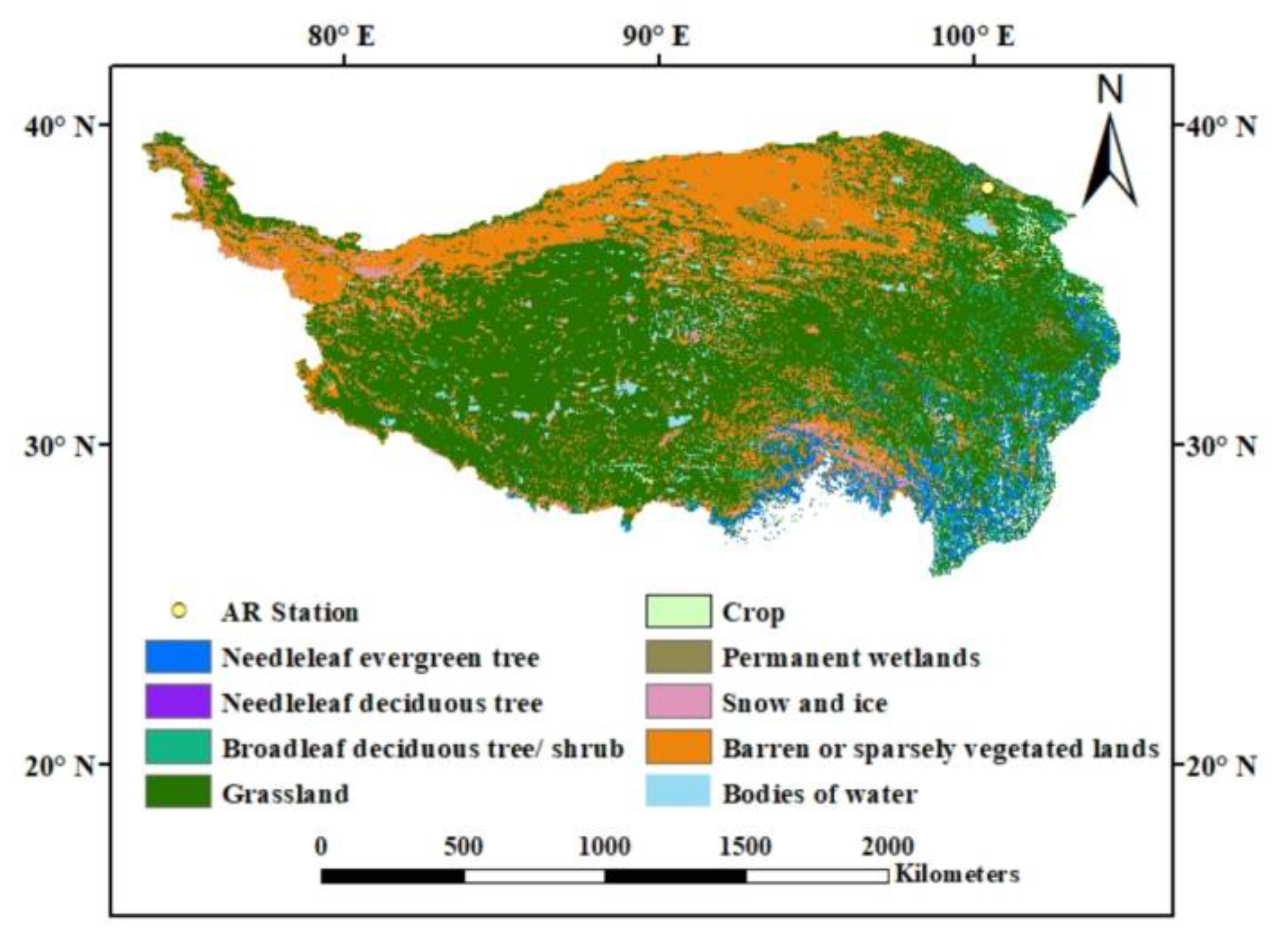
2.1. Study Area
2.2. Meteorological Data
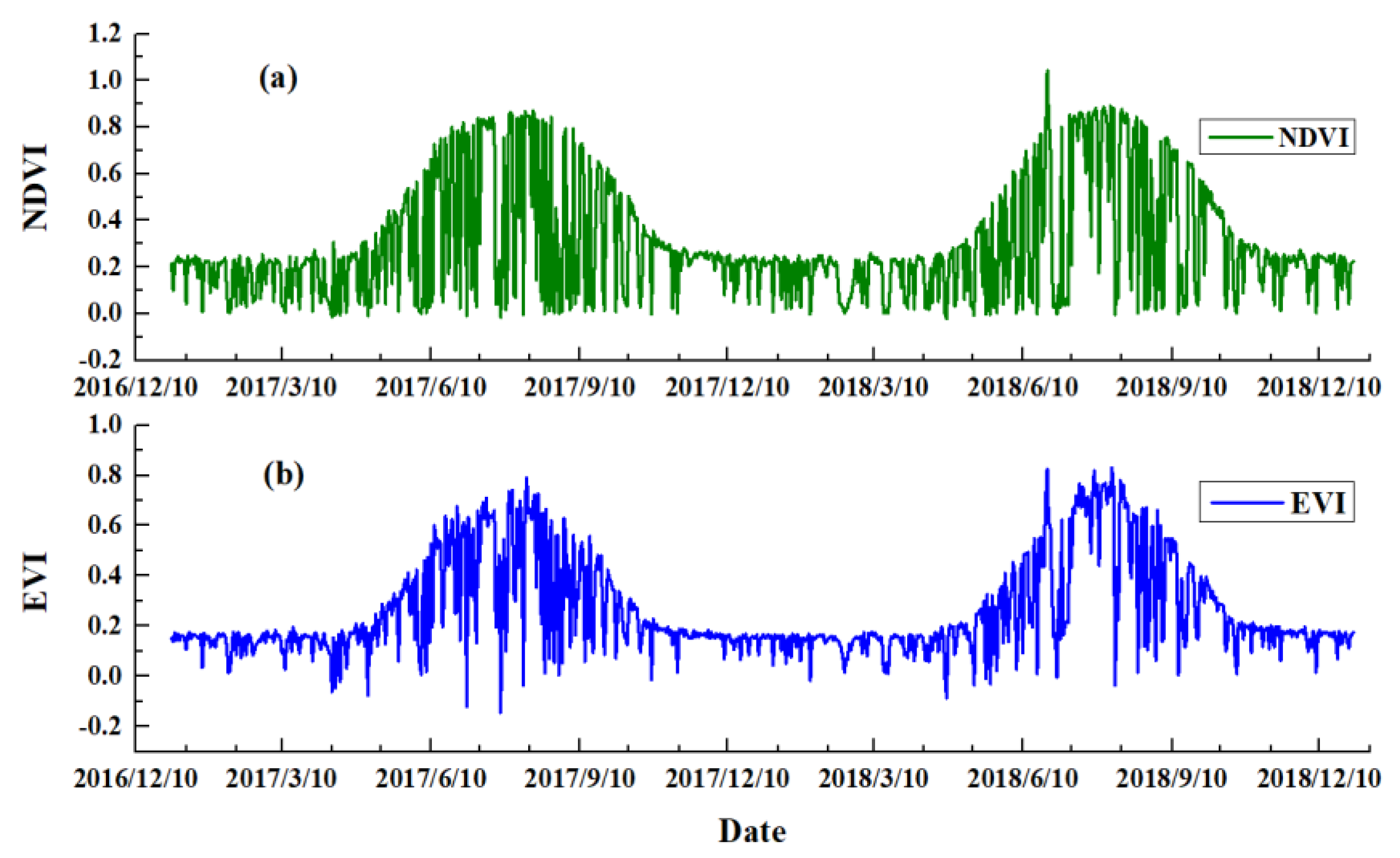
2.3. Remote Sensing Data
2.4. GPP from Eddy Covariance
2.5. Phenological Camera Photos and Color Index Extraction
2.6. GPP Model Based on VIs and GCC
2.7. BP Neural Network Algorithm
2.8. Model Output Accuracy Evaluation
3. Results
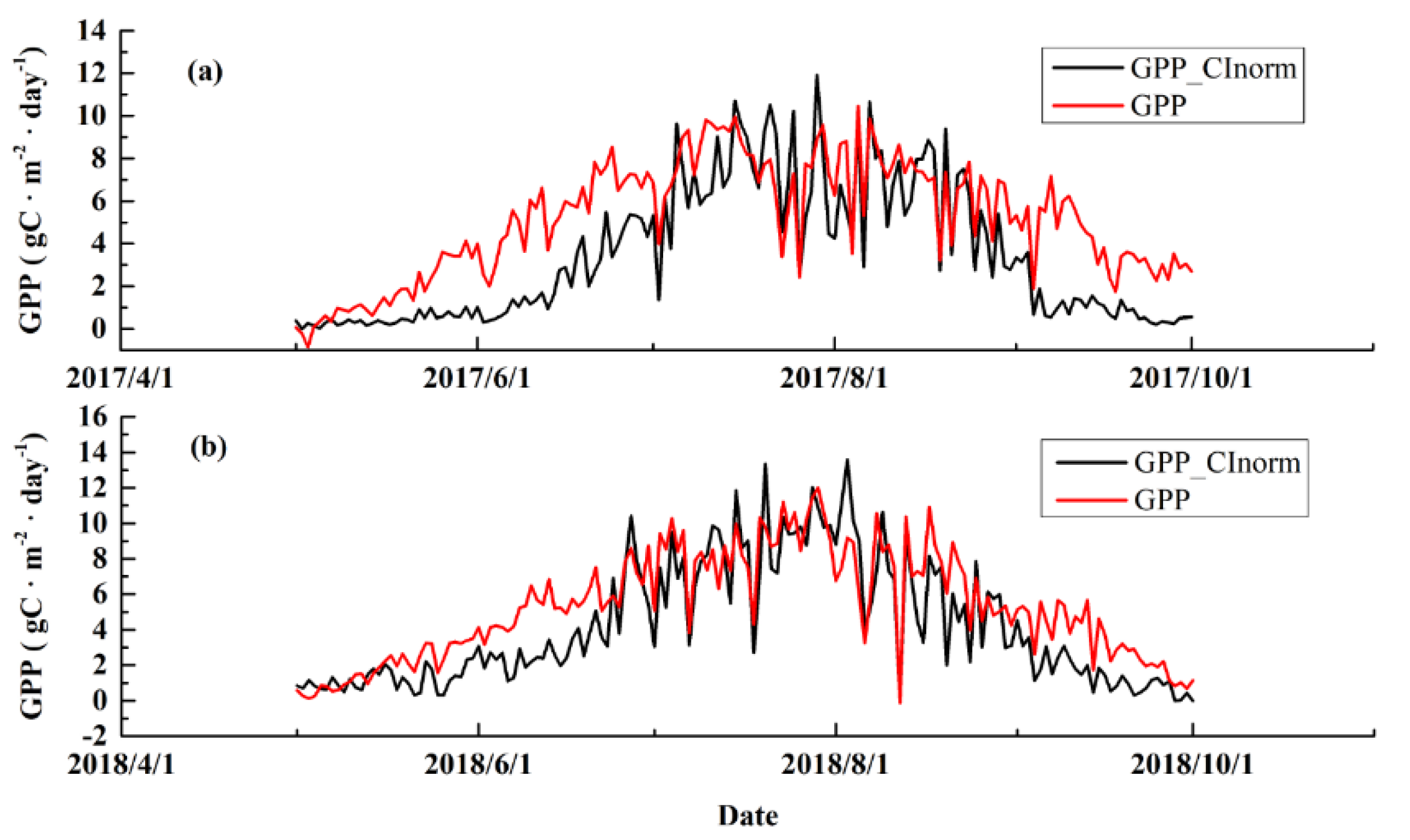
3.1. Simulating GPP with GCC
3.2. Simulating GPP with MOD09GA VIs
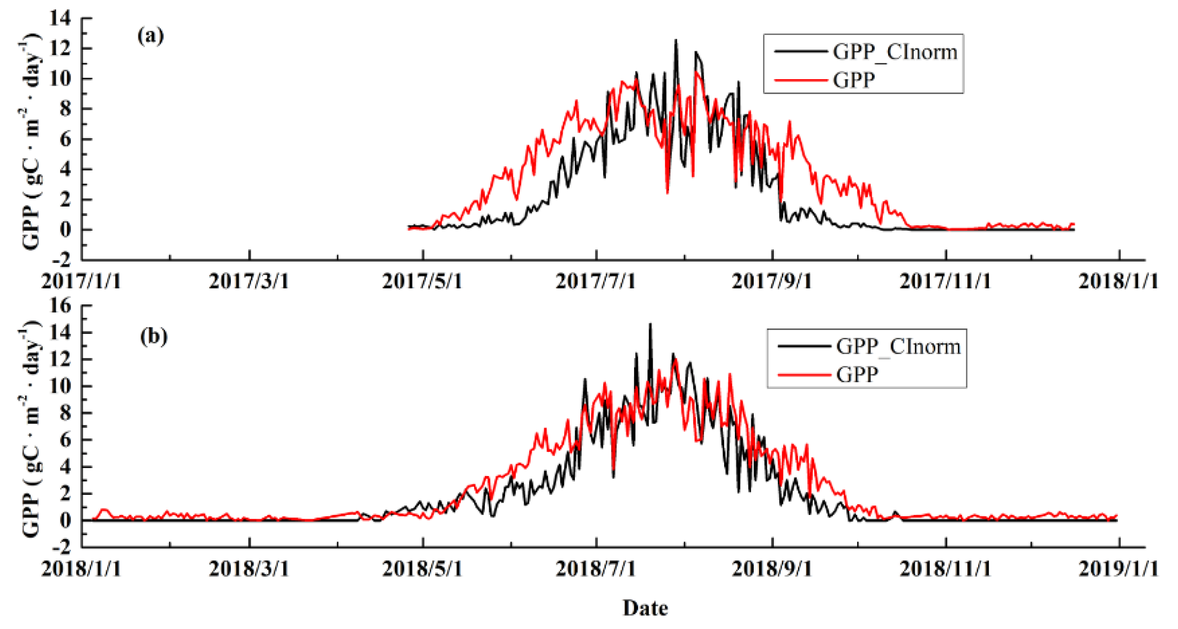
3.3. Simulating GPP with Multisource Data Using Machine Learning
3.4. Comparing the Performance of Different GPP Estimation Methods
4. Discussion
4.1. GPP Estimation Based on GCC
4.2. GPP Estimation Based on Remote Sensing Vegetation Indices
4.3. The Impact of εmax for GPP Estimation
4.4. BNNA Performance Evaluation for GPP Estimation
5. Conclusions
Author Contributions
Funding
Conflicts of Interest
Appendix A


References
- Monteith, J.L. Solar Radiation and Productivity in Tropical Ecosystems. J. Appl. Ecol. 1972, 9, 747–766. [Google Scholar] [CrossRef]
- Wang, S.; Huang, K.; Yan, H.; Yan, H.; Zhou, L.; Wang, H.; Zhang, J.; Yan, J.; Zhao, L.; Wang, Y.; et al. Improving the light use efficiency model for simulating terrestrial vegetation gross primary production by the inclusion of diffuse radiation across ecosystems in China. Ecol. Complex. 2015, 23, 1–13. [Google Scholar] [CrossRef]
- Jia, W.; Liu, M.; Wang, D.; He, H.; Shi, P.; Li, Y.; Wang, Y. Uncertainty in simulating regional gross primary productivity from satellite-based models over northern China grassland. Ecol. Indic. 2018, 88, 134–143. [Google Scholar] [CrossRef]
- Lobell, D.B.; Hicke, J.A.; Asner, G.P.; Field, C.B.; Tucker, C.J.; Los, S.O. Satellite estimates of productivity and light use efficiency in United States agriculture, 1982–1998. Glob. Chang. Biol 2002, 8, 722–735. [Google Scholar] [CrossRef]
- Yu, G.-R.; Zhu, X.-J.; Fu, Y.-L.; He, H.-L.; Wang, Q.-F.; Wen, X.-F.; Li, X.-R.; Zhang, L.-M.; Zhang, L.; Su, W.; et al. Spatial patterns and climate drivers of carbon fluxes in terrestrial ecosystems of China. Glob. Chang. Biol. 2013, 19, 798–810. [Google Scholar] [CrossRef]
- Zhang, W.J.; Wang, H.M.; Yang, F.T.; Yi, Y.H.; Wen, X.F.; Sun, X.M.; Yu, G.R.; Wang, Y.D.; Ning, J.C. Underestimated effects of low temperature during early growing season on carbon sequestration of a subtropical coniferous plantation. Biogeosciences 2011, 8, 1667–1678. [Google Scholar] [CrossRef]
- Mekonnen, Z.A.; Grant, R.F.; Schwalm, C. Contrasting changes in gross primary productivity of different regions of North America as affected by warming in recent decades. Agric. For. Meteorol. 2016, 218–219, 50–64. [Google Scholar] [CrossRef]
- Jahan, N.; Gan, T.Y. Developing a gross primary production model for coniferous forests of northeastern USA from MODIS data. Int. J. Appl. Earth Obs. Geoinf. 2013, 25, 11–20. [Google Scholar] [CrossRef]
- Xiao, J.; Zhuang, Q.; Baldocchi, D.D.; Law, B.E.; Richardson, A.D.; Chen, J.; Oren, R.; Starr, G.; Noormets, A.; Ma, S.; et al. Estimation of net ecosystem carbon exchange for the conterminous United States by combining MODIS and AmeriFlux data. Agric. For. Meteorol. 2008, 148, 1827–1847. [Google Scholar] [CrossRef]
- Wu, C.; Niu, Z.; Gao, S. Gross primary production estimation from MODIS data with vegetation index and photosynthetically active radiation in maize. J. Geophys. Res. 2010, 115. [Google Scholar] [CrossRef]
- Toomey, M.; Friedl, M.A.; Frolking, S.; Hufkens, K.; Klosterman, S.; Sonnentag, O.; Baldocchi, D.D.; Bernacchi, C.J.; Biraud, S.C.; Bohrer, G.; et al. Greenness indices from digital cameras predict the timing and seasonal dynamics of canopy-scale photosynthesis. Ecol. Appl. 2015, 25, 99–115. [Google Scholar] [CrossRef] [PubMed]
- Potter, C.S.; Randerson, J.T.; Field, C.B.; Matson, P.A.; Vitousek, P.M.; Mooney, H.A.; Klooster, S.A. Terrestrial ecosystem production: A process model based on global satellite and surface data. Glob. Biogeochem. Cycle 1993, 7, 811–841. [Google Scholar] [CrossRef]
- Prince, S.D.; Goward, S.N. Global Primary Production: A Remote Sensing Approach. J. Biogeogr. 1995, 22, 815–835. [Google Scholar] [CrossRef]
- Xiao, X.; Hollinger, D.; Aber, J.; Goltz, M.; Davidson, E.A.; Zhang, Q.; Moore, B. Satellite-based modeling of gross primary production in an evergreen needleleaf forest. Remote Sens. Environ. 2004, 89, 519–534. [Google Scholar] [CrossRef]
- Yuan, W.; Liu, S.; Zhou, G.; Zhou, G.; Tieszen, L.L.; Baldocchi, D.; Bernhofer, C.; Gholz, H.; Goldstein, A.H.; Goulden, M.L.; et al. Deriving a light use efficiency model from eddy covariance flux data for predicting daily gross primary production across biomes. Agric. For. Meteorol. 2007, 143, 189–207. [Google Scholar] [CrossRef]
- Sjöström, M.; Ardö, J.; Arneth, A.; Boulain, N.; Cappelaere, B.; Eklundh, L.; de Grandcourt, A.; Kutsch, W.L.; Merbold, L.; Nouvellon, Y.; et al. Exploring the potential of MODIS EVI for modeling gross primary production across African ecosystems. Remote Sens. Environ. 2011, 115, 1081–1089. [Google Scholar] [CrossRef]
- Lin, X.; Chen, B.; Chen, J.; Zhang, H.; Sun, S.; Xu, G.; Guo, L.; Ge, M.; Qu, J.; Li, L.; et al. Seasonal fluctuations of photosynthetic parameters for light use efficiency models and the impacts on gross primary production estimation. Agric. For. Meteorol. 2017, 236, 22–35. [Google Scholar] [CrossRef]
- Montero, P.; Daneri, G.; González, H.E.; Iriarte, J.L.; Tapia, F.J.; Lizárraga, L.; Sanchez, N.; Pizarro, O. Seasonal variability of primary production in a fjord ecosystem of the Chilean Patagonia: Implications for the transfer of carbon within pelagic food webs. Cont. Shelf Res. 2011, 31, 202–215. [Google Scholar] [CrossRef]
- Richardson, A.D.; Braswell, B.H.; Hollinger, D.Y.; Jenkins, J.P.; Ollinger, S.V.J.E.A. Near-surface remote sensing of spatial and temporal variation in canopy phenology. Ecol. Appl. 2009, 19, 1417–1428. [Google Scholar] [CrossRef]
- Sonnentag, O.; Hufkens, K.; Teshera-Sterne, C.; Young, A.M.; Friedl, M.; Braswell, B.H.; Milliman, T.; O’Keefe, J.; Richardson, A.D.J.A.; Meteorology, F. Digital repeat photography for phenological research in forest ecosystems. Agric. For. Meteorol. 2012, 152, 159–177. [Google Scholar] [CrossRef]
- Delpierre, N.; Soudani, K.; Berveiller, D.; Dufrêne, E.; Hmimina, G.; Vincent, G. “Green pointillism”: Detecting the within-population variability of budburst in temperate deciduous trees with phenological cameras. Int. J. Biometeorol. 2020, 64, 663–670. [Google Scholar] [CrossRef] [PubMed]
- Alberton, B.; Torres, R.d.S.; Cancian, L.F.; Borges, B.D.; Almeida, J.; Mariano, G.C.; Santos, J.D.; Morellato, L.P.C. Introducing digital cameras to monitor plant phenology in the tropics: Applications for conservation. Perspect. Ecol. Conser 2017, 15, 82–90. [Google Scholar] [CrossRef]
- Westergaard-Nielsen, A.; Lund, M.; Hansen, B.U.; Tamstorf, M.P. Camera derived vegetation greenness index as proxy for gross primary production in a low Arctic wetland area. ISPRS J. Photogramm. Remote Sens 2013, 86, 89–99. [Google Scholar] [CrossRef]
- Wang, H.; Jia, G.; Epstein, H.E.; Zhao, H.; Zhang, A. Integrating a PhenoCam-derived vegetation index into a light use efficiency model to estimate daily gross primary production in a semi-arid grassland. Agric. For. Meteorol. 2020, 288–289, 107983. [Google Scholar] [CrossRef]
- Zhao, J.; Zhang, Y.; Tan, Z.; Song, Q.; Liang, N.; Yu, L.; Zhao, J. Using digital cameras for comparative phenological monitoring in an evergreen broad-leaved forest and a seasonal rain forest. Ecol. Infor. 2012, 10, 65–72. [Google Scholar] [CrossRef]
- Saitoh, T.M.; Nagai, S.; Saigusa, N.; Kobayashi, H.; Suzuki, R.; Nasahara, K.N.; Muraoka, H. Assessing the use of camera-based indices for characterizing canopy phenology in relation to gross primary production in a deciduous broad-leaved and an evergreen coniferous forest in Japan. Ecol. Infor. 2012, 11, 45–54. [Google Scholar] [CrossRef]
- Wang, M.; Sun, R.; Zhu, A.; Xiao, Z. Evaluation and Comparison of Light Use Efficiency and Gross Primary Productivity Using Three Different Approaches. Remote Sens. 2020, 12, 1003. [Google Scholar] [CrossRef]
- Wolanin, A.; Camps-Valls, G.; Gómez-Chova, L.; Mateo-García, G.; van der Tol, C.; Zhang, Y.; Guanter, L. Estimating crop primary productivity with Sentinel-2 and Landsat 8 using machine learning methods trained with radiative transfer simulations. Remote Sens. Environ. 2019, 225, 441–457. [Google Scholar] [CrossRef]
- Yang, F.; Ichii, K.; White, M.A.; Hashimoto, H.; Michaelis, A.R.; Votava, P.; Zhu, A.X.; Huete, A.; Running, S.W.; Nemani, R.R. Developing a continental-scale measure of gross primary production by combining MODIS and AmeriFlux data through Support Vector Machine approach. Remote Sens. Environ. 2007, 110, 109–122. [Google Scholar] [CrossRef]
- Tramontana, G.; Ichii, K.; Camps-Valls, G.; Tomelleri, E.; Papale, D. Uncertainty analysis of gross primary production upscaling using Random Forests, remote sensing and eddy covariance data. Remote Sens. Environ. 2015, 168, 360–373. [Google Scholar] [CrossRef]
- Lee, B.; Kim, E.; Lim, J.-H.; Kang, M.; Kim, J. Application of Machine Learning Algorithm and Remote-sensed Data to Estimate Forest Gross Primary Production at Multi-sites Level. Korean J. Remote Sens 2019, 35, 1117–1132. [Google Scholar] [CrossRef]
- Du, M.; Kawashima, S.; Yonemura, S.; Zhang, X.; Chen, S. Mutual influence between human activities and climate change in the Tibetan Plateau during recent years. Glob. Planet. Chang. 2004, 41, 241–249. [Google Scholar] [CrossRef]
- Zheng, Z.; Zhu, W.; Chen, G.; Jiang, N.; Fan, D.; Zhang, D. Continuous but diverse advancement of spring-summer phenology in response to climate warming across the Qinghai-Tibetan Plateau. Agric. For. Meteorol. 2016, 223, 194–202. [Google Scholar] [CrossRef]
- An, S.; Chen, X.; Zhang, X.; Lang, W.; Ren, S.; Xu, L. Precipitation and Minimum Temperature are Primary Climatic Controls of Alpine Grassland Autumn Phenology on the Qinghai-Tibet Plateau. Remote Sens. 2020, 12, 431. [Google Scholar] [CrossRef]
- Huete, A.R.; Liu, H.Q.; Batchily, K.; van Leeuwen, W. A comparison of vegetation indices over a global set of TM images for EOS-MODIS. Remote Sens. Environ. 1997, 59, 440–451. [Google Scholar] [CrossRef]
- Shokr, M. Potential directions for applications of satellite earth observations data in Egypt. Egyptian. J. Remote Sens. Space Sci. 2011, 14, 1–13. [Google Scholar] [CrossRef][Green Version]
- Liu, S.M.; Xu, Z.W.; Wang, W.Z.; Jia, Z.Z.; Zhu, M.J.; Bai, J.; Wang, J.M. A comparison of eddy-covariance and large aperture scintillometer measurements with respect to the energy balance closure problem. Hydrol. Earth Syst. Sci. 2011, 15, 1291–1306. [Google Scholar] [CrossRef]
- Gilmanov, T.G.; Soussana, J.F.; Aires, L.; Allard, V.; Ammann, C.; Balzarolo, M.; Barcza, Z.; Bernhofer, C.; Campbell, C.L.; Cernusca, A.; et al. Partitioning European grassland net ecosystem CO2 exchange into gross primary productivity and ecosystem respiration using light response function analysis. Agric. Ecosyst. Environ. 2007, 121, 93–120. [Google Scholar] [CrossRef]
- Wang, X.; Ma, M.; Huang, G.; Veroustraete, F.; Zhang, Z.; Song, Y.; Tan, J. Vegetation primary production estimation at maize and alpine meadow over the Heihe River Basin, China. Int. J. Appl. Earth Obs. Geoinf. 2012, 17, 94–101. [Google Scholar] [CrossRef]
- Ahrends, H.E.; Etzold, S.; Kutsch, W.L.; Stoeckli, R.; Bruegger, R.; Jeanneret, F.; Wanner, H.; Buchmann, N.; Eugster, W. Tree phenology and carbon dioxide fluxes: Use of digital photography for process-based interpretation at the ecosystem scale. Clim. Res. 2009, 39, 261–274. [Google Scholar] [CrossRef]
- Knox, S.H.; Dronova, I.; Sturtevant, C.; Oikawa, P.Y.; Matthes, J.H.; Verfaillie, J.; Baldocchi, D. Using digital camera and Landsat imagery with eddy covariance data to model gross primary production in restored wetlands. Agric. For. Meteorol. 2017, 237, 233–245. [Google Scholar] [CrossRef]
- Zhou, R.; Zhang, Y.; Song, Q.; Lin, Y.; Sha, L.; Jin, Y.; Liu, Y.; Fei, X.; Gao, J.; He, Y.; et al. Relationship between gross primary production and canopy colour indices from digital camera images in a rubber (Hevea brasiliensis) plantation, Southwest China. Forest. Ecol. Manag. 2019, 437, 222–231. [Google Scholar] [CrossRef]
- Heinsch, F.A.; Reeves, M.; Votava, P.; Kang, S.; Milesi, C.; Zhao, M.S. User’s Guide GPP and NPP (MOD17A2/A3) Products NASA MODIS Land Algorithm, Version 2.0. 2002. Available online: http://www.ntsg.umt.edu/modis/MOD17UsersGuide.pdf (accessed on 24 December 2008).
- Zhao, H.; Jia, G.; Wang, H.; Zhang, A.; Xu, X. Seasonal and interannual variations in carbon fluxes in East Asia semi-arid grasslands. Sci. Total Environ. 2019, 668, 1128–1138. [Google Scholar] [CrossRef] [PubMed]
- Chai, X.; Shi, P.; Zong, N.; He, Y.; Zhang, X.; Xu, M.; Zhang, J. A growing season climatic index to simulate gross primary productivity and carbon budget in a Tibetan alpine meadow. Ecol. Indic. 2017, 81, 285–294. [Google Scholar] [CrossRef]
- Li, F.; Wang, X.F.; Zhao, J.; Zhang, X.Q.; Zhao, Q.J. A method for estimating the gross primary production of alpine meadows using MODIS and climate data in China. Int. J. Remote Sens. 2013, 34, 8280–8300. [Google Scholar] [CrossRef]
- Li, Z.; Yu, G.; Xiao, X.; Li, Y.; Zhao, X.; Ren, C.; Zhang, L.; Fu, Y. Modeling gross primary production of alpine ecosystems in the Tibetan Plateau using MODIS images and climate data. Remote Sens. Environ. 2007, 107, 510–519. [Google Scholar] [CrossRef]
- Wang, X.; Ma, M.; Li, X.; Song, Y.; Tan, J.; Huang, G.; Zhang, Z.; Zhao, T.; Feng, J.; Ma, Z.; et al. Validation of MODIS-GPP product at 10 flux sites in northern China. Int. J. Remote Sens. 2013, 34, 587–599. [Google Scholar] [CrossRef]
- Turner, D.P.; Ritts, W.D.; Zhao, M.; Kurc, S.A.; Running, S.W.J.I.T.o.G.; Sensing, R. Assessing Interannual Variation in MODIS-Based Estimates of Gross Primary Production. IEEE Trans. Geosci. Remote Sens. 2006, 44, 1899–1907. [Google Scholar] [CrossRef]
- Xin, Q.; Broich, M.; Suyker, A.E.; Yu, L.; Gong, P. Multi-scale evaluation of light use efficiency in MODIS gross primary productivity for croplands in the Midwestern United States. Agric. For. Meteorol. 2015, 201, 111–119. [Google Scholar] [CrossRef]
- Wei, S.; Yi, C.; Wei, F.; Hendrey, G. A global study of GPP focusing on light-use efficiency in a random forest regression model. Ecosphere 2017, 8. [Google Scholar] [CrossRef]
- Zheng, Y.; Zhang, L.; Xiao, J.; Yuan, W.; Yan, M.; Li, T.; Zhang, Z. Sources of uncertainty in gross primary productivity simulated by light use efficiency models: Model structure, parameters, input data, and spatial resolution. Agric. For. Meteorol. 2018, 263, 242–257. [Google Scholar] [CrossRef]
- Xu, L.; Zhang, X.; Shi, P.; Yu, G. Response of canopy quantum yield of alpine meadow to temperature under low atmospheric pressure on Tibetan Plateau. Sci. China Ser. D Earth Sci. 2006, 49, 219–225. [Google Scholar] [CrossRef]
- Wang, H.; Jia, G.; Fu, C.; Feng, J.; Zhao, T.; Ma, Z. Deriving maximal light use efficiency from coordinated flux measurements and satellite data for regional gross primary production modeling. Remote Sens. Environ. 2010, 114, 2248–2258. [Google Scholar] [CrossRef]


| Parameters and Values | Explanatory Notes |
|---|---|
| epochs = 100 | Number of iterations |
| batch_size = 6 | Number of feeding data for each training model |
| learnrate = 0.1 | Learning rate |
| Activation = “tanh” | Activation function |
| Terror = 1 × 10⁻⁷ | Iteration stop condition |
| Loss = ‘mean_squared_error’ | Loss function |
| Dropout = 0.2 | Rejection rate of each layer |
| model | Hierarchical model |
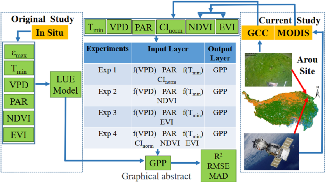
| Experiments | Input Layer | Output Layer |
|---|---|---|
| Exp 1 | f(VPD), PAR, f(Tmin), CInorm | GPP |
| Exp 2 | f(VPD), PAR, f(Tmin), NDVI | GPP |
| Exp 3 | f(VPD), PAR, f(Tmin), EVI | GPP |
| Exp 4 | f(VPD), PAR, f(Tmin), CInorm, NDVI, EVI | GPP |
| GPP | R2 | RMSE | MAD | ||||
|---|---|---|---|---|---|---|---|
| GPP_CInorm | 2017 | 2018 | 2017 | 2018 | 2017 | 2018 | |
| Spring | 0.53 | 0.38 | 1.56 | 1.16 | 1.24 | 0.95 | |
| Summer | 0.55 | 0.75 | 2.77 | 2.07 | 2.44 | 1.80 | |
| Autumn | 0.70 | 0.71 | 2.55 | 2.16 | 2.20 | 1.88 | |
| GPP_NDVI | Spring | 0.32 | 0.24 | 1.12 | 1.34 | 0.85 | 1.08 |
| Summer | 0.29 | 0.34 | 3.80 | 4.07 | 2.94 | 3.12 | |
| Autumn | 0.36 | 0.49 | 3.52 | 3.10 | 2.84 | 2.46 | |
| GPP_EVI | Spring | 0.51 | 0.38 | 0.88 | 1.25 | 0.61 | 0.99 |
| Summer | 0.42 | 0.49 | 3.18 | 3.46 | 2.57 | 2.82 | |
| Autumn | 0.49 | 0.57 | 3.14 | 2.76 | 2.61 | 2.23 | |
| Experiment | Season | R2 | RMSE | MAD | |||
|---|---|---|---|---|---|---|---|
| Training | Validation | Training | Validation | Training | Validation | ||
| 1 | Spring | 0.17 | 0.15 | 1.90 | 2.22 | 1.64 | 1.90 |
| Summer | 0.64 | 0.58 | 1.50 | 1.61 | 1.19 | 1.27 | |
| Autumn | 0.66 | 0.78 | 1.48 | 1.31 | 1.12 | 1.03 | |
| 2 | Spring | 0.53 | 0.29 | 2.62 | 2.18 | 2.38 | 1.83 |
| Summer | 0.42 | 0.35 | 1.80 | 1.90 | 1.45 | 1.59 | |
| Autumn | 0.43 | 0.69 | 1.66 | 1.48 | 1.35 | 1.16 | |
| 3 | Spring | 0.60 | 0.37 | 2.10 | 1.67 | 1.87 | 1.35 |
| Summer | 0.48 | 0.41 | 1.69 | 1.86 | 1.39 | 1.56 | |
| Autumn | 0.47 | 0.65 | 1.63 | 1.63 | 1.26 | 1.26 | |
| 4 | Spring | 0.36 | 0.30 | 1.37 | 1.58 | 1.20 | 1.33 |
| Summer | 0.66 | 0.58 | 1.51 | 1.62 | 1.23 | 1.30 | |
| Autumn | 0.66 | 0.70 | 1.43 | 1.41 | 1.00 | 1.09 | |
| Date/Experiment | GPP | R2 | MAD | RMSE | |
|---|---|---|---|---|---|
| LUE model | 2017 | GPP_CInorm | 0.69 | 2.06 | 2.46 |
| 2018 | GPP_CInorm | 0.78 | 1.64 | 1.95 | |
| 2017 | GPP_NDVI | 0.37 | 2.45 | 3.29 | |
| 2018 | GPP_NDVI | 0.47 | 2.41 | 3.28 | |
| 2017 | GPP_EVI | 0.54 | 2.18 | 2.83 | |
| 2018 | GPP_EVI | 0.59 | 2.19 | 2.84 | |
| Machine Learning Normalized | Training | GPP_train1 | 0.67 | 1.28 | 1.61 |
| Training | GPP_train2 | 0.54 | 1.61 | 1.96 | |
| Training | GPP_train3 | 0.62 | 1.45 | 1.77 | |
| Training | GPP_train4 | 0.73 | 1.15 | 1.47 | |
| Validation | GPP_valid1 | 0.73 | 1.34 | 1.69 | |
| Validation | GPP_valid2 | 0.66 | 1.49 | 1.83 | |
| Validation | GPP_valid3 | 0.69 | 1.41 | 1.74 | |
| Validation | GPP_valid4 | 0.75 | 1.25 | 1.56 |
Publisher’s Note: MDPI stays neutral with regard to jurisdictional claims in published maps and institutional affiliations. |
© 2020 by the authors. Licensee MDPI, Basel, Switzerland. This article is an open access article distributed under the terms and conditions of the Creative Commons Attribution (CC BY) license (http://creativecommons.org/licenses/by/4.0/).
Share and Cite
Zhou, X.; Wang, X.; Zhang, S.; Zhang, Y.; Bai, X. Combining Phenological Camera Photos and MODIS Reflectance Data to Predict GPP Daily Dynamics for Alpine Meadows on the Tibetan Plateau. Remote Sens. 2020, 12, 3735. https://doi.org/10.3390/rs12223735
Zhou X, Wang X, Zhang S, Zhang Y, Bai X. Combining Phenological Camera Photos and MODIS Reflectance Data to Predict GPP Daily Dynamics for Alpine Meadows on the Tibetan Plateau. Remote Sensing. 2020; 12(22):3735. https://doi.org/10.3390/rs12223735
Chicago/Turabian StyleZhou, Xuqiang, Xufeng Wang, Songlin Zhang, Yang Zhang, and Xuejie Bai. 2020. "Combining Phenological Camera Photos and MODIS Reflectance Data to Predict GPP Daily Dynamics for Alpine Meadows on the Tibetan Plateau" Remote Sensing 12, no. 22: 3735. https://doi.org/10.3390/rs12223735
APA StyleZhou, X., Wang, X., Zhang, S., Zhang, Y., & Bai, X. (2020). Combining Phenological Camera Photos and MODIS Reflectance Data to Predict GPP Daily Dynamics for Alpine Meadows on the Tibetan Plateau. Remote Sensing, 12(22), 3735. https://doi.org/10.3390/rs12223735