Determining Optimal Location for Mangrove Planting Using Remote Sensing and Climate Model Projection in Southeast Asia

Abstract

The decreasing area of mangroves is an ongoing problem since, between 1980 and 2005, one-third of the world’s mangroves were lost. Rehabilitation and restoration strategies are required to address this situation. However, mangroves do not always respond well to these strategies and have high mortality due to several growth limiting parameters. This study developed a land suitability map for new mangrove plantations in different Southeast Asian countries for both current and future climates at a 250-m resolution. Hydrodynamic, geomorphological, climatic, and socio-economic parameters and three representative concentration pathway (RCP) scenarios (RCP 2.6, 4.5, and 8.5) for 2050 and 2070 with two global climate model datasets (the Centre National de Recherches Météorologiques Climate model version 5 [CNRM-CM5.1] and the Model for Interdisciplinary Research on Climate [MIROC5]) were used to predict suitable areas for mangrove planting. An analytical hierarchy process (AHP) was used to determine the level of importance for each parameter. To test the accuracy of the results, the mangrove land suitability analysis were further compared using different weights in every parameter. The sensitivity test using the Wilcoxon test was also carried out to test which variables had changed with the first weight and the AHP weight. The land suitability products from this study were compared with those from previous studies. The differences in land suitability for each country in Southeast Asia in 2050 and 2070 to analyze the differences in each RCP scenario and their effects on the mangrove land suitability were also assessed. Currently, there is 398,000 ha of potentially suitable land for mangrove planting in Southeast Asia, and this study shows that it will increase between now and 2070. Indonesia account for 67.34% of the total land area in the “very suitable” and “suitable” class categories. The RCP 8.5 scenario in 2070, with both the MIROC5 and CNRM-CM5.1 models, resulted in the largest area of a “very suitable” class category for mangrove planting. This study provides information for the migration of mangrove forests to the land, alleviating many drawbacks, especially for ecosystems.

1. Introduction

Mangroves are defined as the vegetation that grows along the intertidal zones in both tropical and subtropical countries [1,2,3,4], and they are beneficial for humans and their surrounding ecosystems. For example, they can protect people from natural hazards, such as storm surges and tsunamis [5,6,7], act as water purifiers, and prevent coastal erosion and abrasion [5]. Furthermore, mangrove ecosystems have an important functional role in determining the balance of biological and nutrient cycling [8,9,10] since they are often used as nursery habitats [9,10]. Moreover, they play a significant role in preventing climate change, as they sequester 1.023 Mg of carbon per hectare [5,8] and have five times the carbon of tropical, boreal, and temperate forests [11].

In the 20th century, mangroves covered approximately 181,000 km² globally [12], and almost half of the world’s current mangroves are in Asia [12,13]. However, according to the Food and Agriculture Organization (FAO; 14), approximately one-third of the global mangrove area was lost from 1980 to 2005, and, from this, the largest loss was in Asia [14]. In Southeast Asia, more than 110,000 ha of mangroves have been deforested of which approximately 97,000 ha were lost from 2000 to 2012 [15]. Over half the known mangrove species (36 and 46 out of 70) are found in the Indo-Malay Philippine Archipelago [16]. In these regions, less than 15% of the mangrove species are threatened [16].

Anthropogenic activities are one of the main factors leading to the decline of mangrove areas [8,15]. According to Richards and Friess (2016, [15]), the conversion of mangroves into aquaculture and rice fields is the biggest cause of mangrove deforestation in Southeast Asia. Additionally, climate change is also causing loss in some areas because of drought, sea level rise, and a drastic increase in temperature and salinity, to which mangroves find it difficult to adapt [17,18,19]. For instance, during the transition from El Niño to La Niña in 2016, the mortality rate of seedlings increased dramatically, owing to an increase in the salinity levels and the tidal inundation on the Pacific coast of Columbia [20]. The loss of mangroves has many negative consequences, and, for some countries, results in economic decline [5,21]. For example, the decrease of mangrove areas in the Gulf of California is predicted to reduce the productivity of fish and crabs by approximately 37,500 USD per hectare [21]. Furthermore, mangrove loss can also disrupt coastal ecosystems [5].

Rehabilitation and restoration strategies are required to address the global decreases in mangrove areas [5,6,22]. However, some mangroves do not respond well to these strategies and have high mortality rates, owing to several parameters that hinder their growth [23,24,25,26,27,28,29,30]. For example, in the Philippines, during mangrove rehabilitation practices, seedlings experienced a mortality rate of 10%–20% because of unsuitability of the location selected [25]. This highlights one of the main reasons for mangrove restoration failures, as unsuitable target areas often do not have the required tidal inundation for mangrove growth [24,26]. The presence of high waves erodes the coastal area and can result in the death of new mangrove plants [23,28]. According to previous investigations [31], the beach slope and elevation affect the frequency of tidal inundation and the impact strength of the waves. This indicates that the elevation and slope parameters are important when selecting suitable areas for mangrove restoration. In addition, in Fujian and Zhejiang, the failure of mangrove rehabilitation was partly due to their unsuitable climates [32].

Two of the important climatic parameters for mangrove growth are precipitation and air temperature. Future climate models project that there will be extreme variations in precipitation [33,34]. Schewe and Levermann (2012, [35]) have predicted that an increase in temperature at the end of the 21st century and early 22nd, will cause changes in the distribution of rainy seasons to 70% below normal. This will cause the rainy seasons in Southeast Asia to be delayed [36,37]. Changes in precipitation can affect the growth, distribution, and area of mangroves [17]. According to Fischer and Knutti [38], an increase in precipitation will result in the death of plants. Conversely, Eslami-Andargoli et al. [39] found that an increase in precipitation could increase the number of mangrove areas due to the expansion of mangrove forests inland. Increases in precipitation could also lead to decreases in pore water salinity and sulfate concentrations, which could increase mangrove productivity [40]. In addition, future climate models also project that there will be an increase in air temperature of 10% °C⁻¹ in Southeast Asia [41,42]. According to the Intergovernmental Panel on Climate Change (IPCC) (2013, [34]), with scenario representative concentration pathway 8.5 (RCP 8.5), global temperatures are expected to increase by 4.8 °C from 2081–2100. An increase in temperature will affect the rate of evaporation and transpiration, which adversely affects plants [43]. Furthermore, a decrease in precipitation and an increase in evaporation will cause an increase in soil salinity. This will result in decreased seedling survival and increase mangrove loss, as their current areas will become hypersaline mud plains [19,44,45]. The occurrence of increased salinity and drought may also affect the species diversity, size, and productivity of mangrove forests [46,47]. Research is, thus, required to identify suitable areas for mangrove restoration in future climatic conditions using various RCP scenarios in Southeast Asia. Moreover, social and economic factors also greatly influence the selection of land for mangrove restoration. This is because coastal urban areas have grown at a faster rate than non-urban coastal areas [48,49]. The coastal population growth and rate of urbanization, which have outpaced demographic development in inland areas, have been driven by rapid economic growth and migration to the coast [50,51]. Hence, the existence of rapid population growth and a coastal economy are important parameters to consider when identifying suitable land for mangrove restoration.

Remote sensing techniques, such as mapping and monitoring, have been used extensively in mangrove research. For example, Vo et al. and Zhen et al. [52,53] used remote sensing to map mangrove forests, whereas Liu et al. and Fauzi et al. [54,55] used remote sensing to monitor the changes in mangrove forests and analyze the cause of their deforestation. Once potential areas have been identified using methods like remote sensing, their suitability needs to be ranked so the optimal areas can be selected for rehabilitation and restoration [56,57]. There are several weighting techniques for land suitability analysis, such as artificial neural networks [58,59], multivariate applications [60], multi-criteria analysis outperforming competitors [61], boolean classification methods [62], root quadratic and multilevel methods [63,64], productivity index [65], a pairwise comparison matrix [66], and an analytical hierarchy process (AHP) [67,68,69,70,71,72,73,74,75,76,77,78]. This study utilized AHP as its weighting method. AHP is a model that is widely used in decision-making processes, such as when selecting potential land areas and calculating their risk and vulnerability [56,57,58,59,60,61,62,63,64,65,66,67,68,69,70,71,72,73,74,75,76,77,78].The large number of recent investigations into mangroves makes the AHP model the most suitable for this investigation. This is because this method uses the criteria suggested in previous studies and expert opinions to decide the weight of each of its own criterion. In addition, AHP can consider the relative priority of alternatives as well as represent the best alternative, as it determines the effects of certain weights based on the comparison of paired parameters, according to relative importance [79]. AHP analysis also calculates the consistency value of the index, so that the weights generated for each alternative are consistent with one another [79].

The objective of this study was to assess the amount of land suitable for mangrove restoration today and in the future, according to the different climate change scenarios for 2050 and 2070, using the AHP method with remote sensing, model, and statistical data. The study areas were in Southeast Asia and included Myanmar, Thailand, Cambodia, Vietnam, the Philippines, Malaysia, Singapore, Brunei Darussalam, and Indonesia. To the best of our knowledge, this is the first study to combine climate, hydrodynamic, geomorphological, and socio-economic data to determine the suitability of mangrove land for mangroves in the regional areas using remote sensing, model, and statistical data.

2. Materials and Methods

To determine if the land now, and in the future, is suitable for planting mangroves, this study used hydrodynamic, geomorphological, and climatic parameters. The geomorphological parameters included elevation and slope sub-parameters. The hydrodynamic parameters included tidal inundation sub-parameters, and the climatic parameters included air temperature and precipitation sub-parameters. AHP was used as a method of weighting and determining the importance of each parameter and sub-parameter. After identifying the land suitable for planting mangroves, this study analyzed the socio-economic parameters of the area and their influences on the land’s suitability. The socio-economic parameters represented the human pressures that hinder mangrove restoration and included parameters for land cover, population, gross domestic product (GDP), and night light. To understand the effects of using the AHP method to weigh the selections for mangrove land suitability, the results were compared with the results of the land selection using equal weights (i.e., without AHP). They were also compared with the land suitability products of other studies to analyze the uncertainties in this study. The suitable sites for mangrove growth in 2050 and 2070 were assessed using climate model data (precipitation and average air temperature parameters) from the Centre National de Recherches Météorologiques Climate model version 5 (CNRM-CM5.1) and the Model for Interdisciplinary Research on Climate (MIROC). Three RCP scenarios (RCP 2.6, 4.5, and 8.5) were used for each climate parameter. This study compared the results of the current land suitability with that in 2050 and 2070 for each RCP scenario with the two climate models to determine the differences in each scenario for mangrove planting.

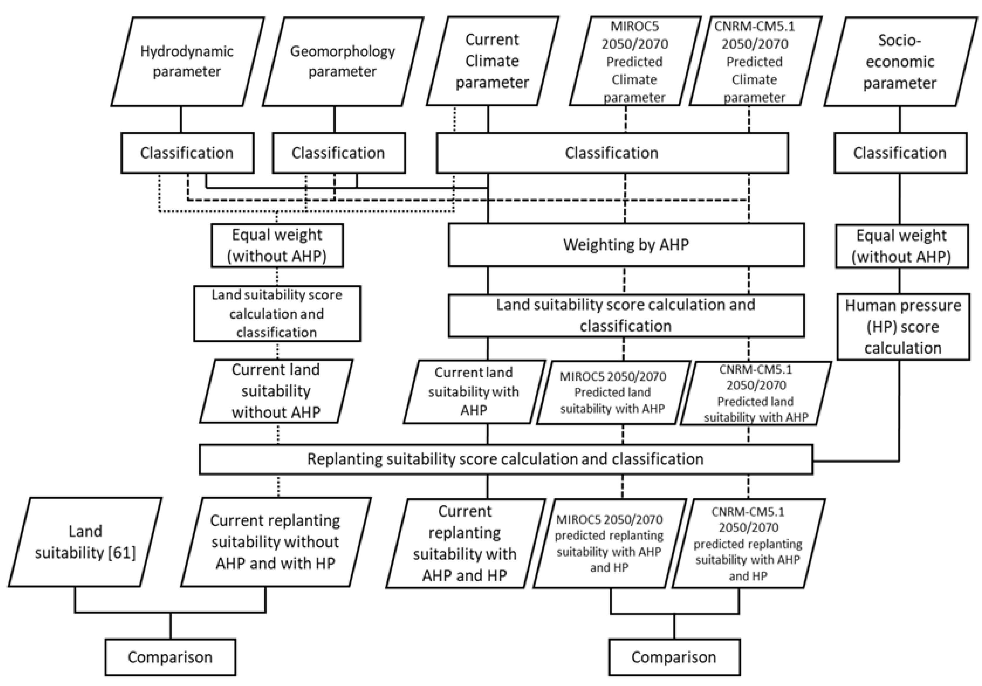
The methodology used in this study was divided into stages. The first stage was to determine the parameters and build their hierarchy. The second stage was to create the base map. The third stage was to classify both the parameters and the sub-parameters into several classes. The fourth stage was to determine the weight of each parameter and sub-parameter using the AHP method. Finally, the fifth stage was to create scenarios to determine the land’s suitability for mangroves. Figure 1 shows the data-processing schemes for the land suitability analysis for mangrove planting.

2.1. Determination of Parameters and Hierarchy Building

The determination of the appropriate parameters was the most important step for identifying land suitability. The parameters were first selected from a literature review and then the parameters were divided into three categories. The first category included the hydrodynamic, geomorphological, and climatic parameters that made the land suitable for planting mangroves. Moreover, the sub-parameters used in this study were those that had the highest weight when compared with the other sub-parameters, when weighted using the AHP method, and those with very low weights were not used in this study. The second category included parameters that make a land unsuitable for planting mangroves, owing to intensive social and economic anthropogenic activities. In this study, these parameters were classified as human pressure parameters. Finally, the third category included climate prediction model parameters. These parameters were used to predict the land suitability for the future growth of mangroves, while assuming that there would be no changes in the hydrodynamic, geomorphological, and human pressure parameters.

2.1.1. Hydrodynamic

The seawater parameter had one sub-parameter, which was tidal inundation. The tidal inundation data used in this study were obtained from tidal data models. The tidal data model was created from TPXO 9.0 data. TPXO is a tidal model based on bathymetry, which assimilates various data sources and is processed using OTIS software [80,81]. The tidal model was verified using tidal station data across Indonesia, which are available from the Indonesian Geospatial Information Agency. Subsequently, the tidal inundation was calculated by multiplying the amplitude value by two, which results in a tidal inundation map of 2018 that had a spatial resolution of 1°.

2.1.2. Geomorphology

The geomorphology parameter had two sub-parameters, elevation, and slope. The elevation and slope sub-parameter data used in this study were obtained from the Multi Error Removed Improved Terrain Digital Elevation Model (MERIT DEM). MERIT DEM is the result of the development of DEM data from SRTM3 v2.1 and AW3D-30m v.1, which eliminated several error components, including absolute bias, noise stripe, noise speckle, and height of the tree bias. These data had a spatial resolution of 90 m [82].

2.1.3. Climate

The climatic parameters had two sub-parameters, namely, average air temperature and precipitation. The average air temperature data used in this study were the 2 m air temperature data obtained from the European Center for Medium-Range Weather Forecasts (ECMWF). These air temperature data pertained to 2 m above the land, sea, or water surface. The 2-m air temperature was calculated by interpolating between the lowest level model and the surface of the earth, while taking atmospheric conditions into account. The unit of measurement for this parameter was kelvin (K). The data used were monthly data derived from daily data accumulation with a spatial resolution of 0.125°.

The precipitation data used in this study were obtained from the Climate Hazards Group InfraRed Precipitation with Stations version 2.0 (CHIRPS v.2.0). The CHIRPS data were a combination of pentadal rainfall data, global geostationary TIR satellite observations from Climate Prediction Center (CPC) and the National Climatic Data Center (NCDC), rainfall atmospheric models from the NOAA Climate Forecast System version 2 (CFSv2), and rainfall data collected from in situ observations at each station [83,84]. This CHIRPS product had a 0.05° spatial resolution with pentadal, decadal, and monthly temporal resolutions [85].

2.1.4. Human Pressure

Human pressure was the parameter that made an area unsuitable for planting mangroves owing to over-population and development of urban areas. The human pressure parameter had four sub-parameters, land cover, population, gross domestic product (GDP), and night light. The land cover data used in this study were climate change land cover initiative (CCI-LC) data from the European Space Agency (ESA). These data describe the surface of the earth in 37 classes of the original land cover based on the United Nations Land Cover Classification System (UN-LCCS) with a spatial resolution of 300 m [86]. The population data used in this study were gridded populations sourced from the world version 4 (GPWv4) data. These data provide information on the population density (number of people per km²) with a 30″ × 30″ grid size [87].

The GDP data used in this study were obtained from Kummu et al. [88]. They included USD GDP data, obtained from the GDP per capita multiplied by the History Database of the Global Environment (HYDE) population data 3.2, which had a grid size of 5′ × 5′ [88]. The night light data used in this study were the black marble nighttime light (VNP46) data of the National Aeronautics and Space Administration (NASA). These data had a spatial resolution of 500 m. NASA developed black marble as a series of daily products that were calibrated, correlated, and validated, so that the night light data could be used effectively for scientific observations [89].

2.1.5. Climate Prediction Model

The climate prediction data model had two sub-parameters, namely, average air temperature and precipitation. These sub-parameters were obtained from the CNRM-CM5.1 and the MIROC5 models. CNRM-CM5.1 and MIROC5 are the earth system models designed to facilitate simulations that contribute to phase five of the Coupled Model Intercomparison Project (CMIP5). CNRM-CM5.1 consists of several models, namely, the atmospheric model from ARPEGE-Climat version 5.2 and the marine model from The Nucleus for European Modelling of the Ocean version 3.2 (NEMO v3.2) and includes the Interaction Sol-Biosphère-Atmosphère (ISBA) land surface and the sea ice model from Global Experimental Leads and sea ice for Atmosphere and Ocean version 5 (GELATO v5). These models were designed independently and combined through OASIS v.3 software [90]. The CNRM-CM5.1 data had a spatial resolution of 1.4° × 1.4° and it is one of the best global climate models for temperature and rainfall parameters data in Southeast Asia [91]. MIROC5 is a climate prediction model created by the Japanese research community. It has 40 standard vertical resolution levels of up to 3 hPa with a spatial resolution of 1.4° × 1.4°. MIROC5 has better climatological features (precipitation, average zonal atmospheric fields, equatorial subsurface fields, and El Niño-Southern Oscillation simulations) than the previous version [92]. Both CNRM-CM5.1 and MIROC5 included three scenarios, namely, RCP 2.6, 4.5, and 8.5. In RCP 2.6, the greenhouse gas concentration was very low, while RCP 4.5 meant that the total radiative forcing was stabilized shortly. In RCP 8.5, the greenhouse gas emissions increase over time, resulting in higher concentrations. In this study, the results of the mangrove suitability site analyses were compared in the context of these RCPs to determine the scenarios that included the most suitable sites for planting mangroves.

2.2. Creation of the Basemap

Before initiating the data processing, a base map was constructed from coastline data and mangrove distributions and buffered 10 km inland. The mangrove distribution data used in this study were obtained from Giri et al. [13]. The primary data for the mangrove distribution resulted from a combination of the global land survey (GLS) data from 1997 to 2000, with a 30-m resolution, and the Landsat imagery available from the United States Geological Survey (USGS). The secondary data used were global mangrove data [14] and data from the national and local mangrove databases. The mangrove distribution data were buffered 10 km inland. This base map was then used for land selection and to analyze land suitability.

2.3. Classification of the Parameter

To select suitable land for planting mangroves, each parameter needed to be classified and scored. The classification and scoring in this study involved two stages. The first stage was the division of the classes of each land suitability parameter. Each parameter could be classified into four classes (very suitable, suitable, moderate, and unsuitable). The classes were devised based on the results of a literature review (

Table 1. Classification of the land suitability and human pressure parameters.

	Parameter	Sub-Parameter	Class Value	Class	Reference
Land suitability parameters	Climate	Air temperature (°C)	28–30	Very suitable	[93]
			26–28, 30–32	Suitable
			8–26, 32–42	Moderate
			<8, >42	Unsuitable
		Precipitation (mm)	1400–3750	Very suitable	[94]
			1200–1400, 3750–4500	Suitable
			0–1200, 4500–7500	Moderate
			>7500	Unsuitable
	Geomorphology	Elevation (m)	(−0.25)–1.5	Very suitable	[95]
			(−0.20)–(−0.25), 1.5–1.8	Suitable
			(−0.20)–(−0.4), 1.8–2.8	Moderate
			<(−0.4), >2.8	Unsuitable
		Slope (%)	0–2	Very suitable	[96]
			2–2.15	Suitable
			2.15–2.5	Moderate
			>2.5	Unsuitable
	Hydrodynamic	Tidal inundation (m)	≤0.4	Very suitable	[97,98]
			0.4–0.3	Suitable
			0.3–1.27	Moderate
			>1.27	Unsuitable
Human pressure parameters	Land cover	-	189–191	Very high	-
			10–189, 191–210	Low
	Population	-	> 150	Very high	-
			50–150	High
			10–50.0	Medium
			<10	Low
	GDP per capita (PPP)	-	>12.375	Very high	[99]
			3.996–12.375	High
			1.026–3.996	Medium
			<1.026	Low
	Nightlight	-	14–255	Very high	-
			10–14.0	High
			7.0–10	Medium
			2.0–7.0	Low

). The second stage involved assigning a score to each class. Very suitable and suitable classes were assigned scores of four and three, respectively, whereas moderate and unsuitable classes were assigned scores of two and one, respectively. In addition, class divisions and scores were applied to each human pressure parameter. The human pressure parameters could be categorized into either of four classes (low, medium, high, and very high) except for the land cover parameter. The land cover parameter included two classes (urban and non-urban). Low, medium, high, and very high classes were assigned scores of one, two, three, and four, respectively.

2.4. Determination of the Parameters Weight

The AHP method was used to determine the parameter weights in this study. AHP is a decision-making technique developed by Saaty [79] and was carried out in three stages. First, a pairwise comparison matrix was created by creating a scale with values from one to nine for the hydrodynamic, geomorphological, and climate parameters (

Table 2. Pairwise comparison matrix to determine the weights of the main parameters.

Parameter	Hydrodynamic	Geomorphology	Climate
Hydrodynamic	1.000	1/3	2.000
Geomorphology	1.000	1.000	2.000
Climate	1.000	1/3	1.000
n = 3, λ = 2.91, CI = −0.046, RI = 0.58, CR = −0.01

). The scale of importance between one parameter and another was determined by expert judgment. Second, normalize the results of the pairwise comparison matrix were normalized and a column vector created that had n units with n components, so that the weight value and the total weight vector for each parameter could be obtained. Third, the consistency ratios were estimated. To calculate the consistency ratio, the lambda (λ) and consistency index (CI) parameters were required. The λ value was the average value of the consistency vector values of all parameters. The consistency vector value was obtained by dividing the number vector by the weight of each parameter with the following formula.

$$\mathrm{Vector}\mathrm{of}\mathrm{consistency}\left(V{C}_{n^{th}parameter}\right)=\frac{Numberofvector{s}_{n^{th}parameter}}{Weigh{t}_{n^{th}parameter}}$$

(1)

$$\mathrm{Average}\mathrm{consistency}\left(\mathsf{\lambda }\right)=\frac{V{C}_{1^{st}parameter}+V{C}_{2^{nd}parameter}+V{C}_{n^{th}parameter}}{Numberofparameters}$$

(2)

The λ value was used to calculate the CI value, as described in Equation (3). The CI calculation was based on the observation that λ is always greater than or equal to the number of the criteria considered (n). If the paired comparison matrix is a consistent matrix, then it has a positive value, a reciprocal matrix, and λ = n. Therefore, if λ-n, then it can be considered as a measure of the inconsistency level. For more details, the CI formula can be written as follows.

$$CI=\frac{\mathsf{\lambda }-n}{n-1}$$

(3)

The CI value in Equation (3) can be used to calculate the consistency ratio (CR), as described in Equation (4) below.

$$CR=\frac{CI}{RI}$$

(4)

where RI (random index) is the consistency index of a paired comparison matrix that is randomly generated. If a CR value of less than 0.10 was obtained, it indicated a level of rational/reasonable consistency in pairwise comparisons. However, if the CR value obtained was greater than 0.10, the ratio values indicated inconsistent ratings. If the assessment was inconsistent, a correction needed to be made to the scoring when the comparison matrix was paired. Table 2 shows the pairwise comparison matrix of the main parameters and the value of the CR from this study. Moreover, pairwise comparison matrixes for the sub-parameters are shown in

Table A1. Pairwise comparison matrix for determination of the weight of hydrodynamic sub-parameters.

Sub-Parameter	Sea Water Temperature	Energy from Sea Wave and Sea Tide	Tidal Inundation
Sea water temperature	1	1/3	1/3
Energy from sea wave and sea tide	3	1	1/3
Tidal inundation	3	2	1
n = 3; λ = 2.965; CI = −0.0177; RI = 0.58; CR = −0.031

,

Table A2. The weight of hydrodynamic sub-parameters.

Sub-Parameter	Weight
Sea water temperature	0.15
Energy from sea wave and sea tide	0.31
Tidal inundation	0.54

,

Table A3. Pairwise comparison matrix for determination of the weight of geomorphology sub-parameters.

Sub-Parameter	Slope	Bathymetry	Elevation
Slope	1.000	3.000	1/3
Bathymetry	1.000	1.000	1/4
Elevation	1.000	2.000	1.000
n = 3; λ = 3.067; CI = 0.034; RI = 0.58; CR = 0.058

,

Table A4. The weight of geomorphology sub-parameters.

Sub-Parameter	Weight
Slope	0.35
Bathymetry	0.22
Elevation	0.43

,

Table A5. Pairwise comparison matrix for determination of the weight of climate sub-parameters.

Sub-Parameter	Air Temperature	Precipitation	Evaporation
Air temperature	1.000	1.000	3.000
Precipitation	1/3	1.000	4.000
Evaporation	1/2	1/4	1.000
n = 3; λ = 3.016; CI = 0.008; RI = 0.58; CR = 0.014

,

Table A6. The weight of climate sub-parameters.

Sub-Parameter	Weight
Air temperature	0.45
Precipitation	0.38
Evaporation	0.17

and

Table A7. The weight of sub-parameters after normalized.

Sub-Parameter	Weight	New weight
Tidal inundation	0.54	0.25
Slope	0.35	0.16
Elevation	0.43	0.20
Air temperature	0.45	0.21
Precipitation	0.38	0.17

. The results of the weighting method using AHP for each parameter and sub-parameter are shown in

Table 3. The weight of each parameter and sub-parameter.

Parameter		Sub-Parameter
Parameter	Weight of Parameter	Sub-Parameter	Weight of Sub-Parameter	Class Value
Climate	0.25	Air temperature (°C)	0.21	28–30
				8–28, 30–42
				6–8, 42–44
				<6, >44
		Precipitation (cm)	0.17	140–375
				0–140, 375–750
				750–850
				>8500
Geomorphology	0.44	Elevation (m)	0.20	(−0.25)–1.5
				(−0.4)–(−0.25), 1.5–2.8
				(−1.5)–(−0.4), 2.9–3.5
				<(−1.5), >3.5
		Slope (%)	0.16	0–2
				2–2.5
				2.5–3
				3.0–4.0
Hydrodynamic	0.31	Tidal inundation (m)	0.25	≤0.4
				0.4–1.27
				1.27–2
				2.0–3.0

.

2.5. Scenario Generation of Land Suitability

In this study, five scenarios were created to analyze the suitability of the land for mangrove planting in Southeast Asia. In the first scenario, a land suitability map for mangrove planting was created with the use of the AHP method. In the second scenario, the AHP method was utilized and the influences of the human pressure parameters were also considered. In the third scenario, all parameters were assumed to have the same level of importance, and the AHP method was not used. The influence of the human pressure parameters was not considered, as described in Equation (5). In the fourth scenario, all parameters were assumed to have the same level of importance, and the influence of the human pressure parameters was considered. Finally, in the fifth scenario, a land suitability map for mangrove planting in 2050 and 2070, using the data from the two models (CNRM-CM5.1 and MIROC5) was constructed with the use of the AHP method and influence of the human pressure parameters, as represented in Equations (6) and (7). The scenarios in which the human pressure parameters were considered aimed to assess their influence and how essential it was to consider them when selecting suitable areas for mangroves. The scenarios that did not utilize AHP were used to determine the accuracy of the weight results obtained from the AHP method based on the subjectivity of the experts’ judgment. To assess the differences between the AHP effects, the Wilcoxon test was carried out as described previously by Chakraborty et al. [57]. The Wilcoxon test can also be used to compare the mean values of a variable from two paired sample data [100,101], whereas the Wilcoxon signed rank test is used only for interval or ratio type data that does not follow a normal distribution. In addition, Equations (5)–(7), respectively, represent the calculations for the replanting suitability of the mangroves’ sites.

$$Replantingsuitabilityscore=Landsuitabilityscore-Humanpressurescore$$

(5)

$$TotalscorewithAHP={\displaystyle \sum }_{i=1}^m(wpi.\hspace{0.17em}{\displaystyle \sum }_{j=1}^n\left(wspij.\hspace{0.17em}wrij\right))$$

(6)

$$TotalscorewithoutAHP={\displaystyle \sum }_{i=1}^m(\frac{1}{m}.\hspace{0.17em}{\displaystyle \sum }_{j=1}^n(\frac{1}{n}.\hspace{0.17em}wspij.\hspace{0.17em}wrij))$$

(7)

where:

m = number of sub-parameters,

n = number of sub-parameters,

wpi = weight of parameter I,

wspij = weight of sub-parameter j in parameter I,

wrij = ranking weight of the pixel’s sub-parameter j class in parameter i.

3. Results

3.1. Land Suitability for Mangrove Planting as Determined with the AHP Method

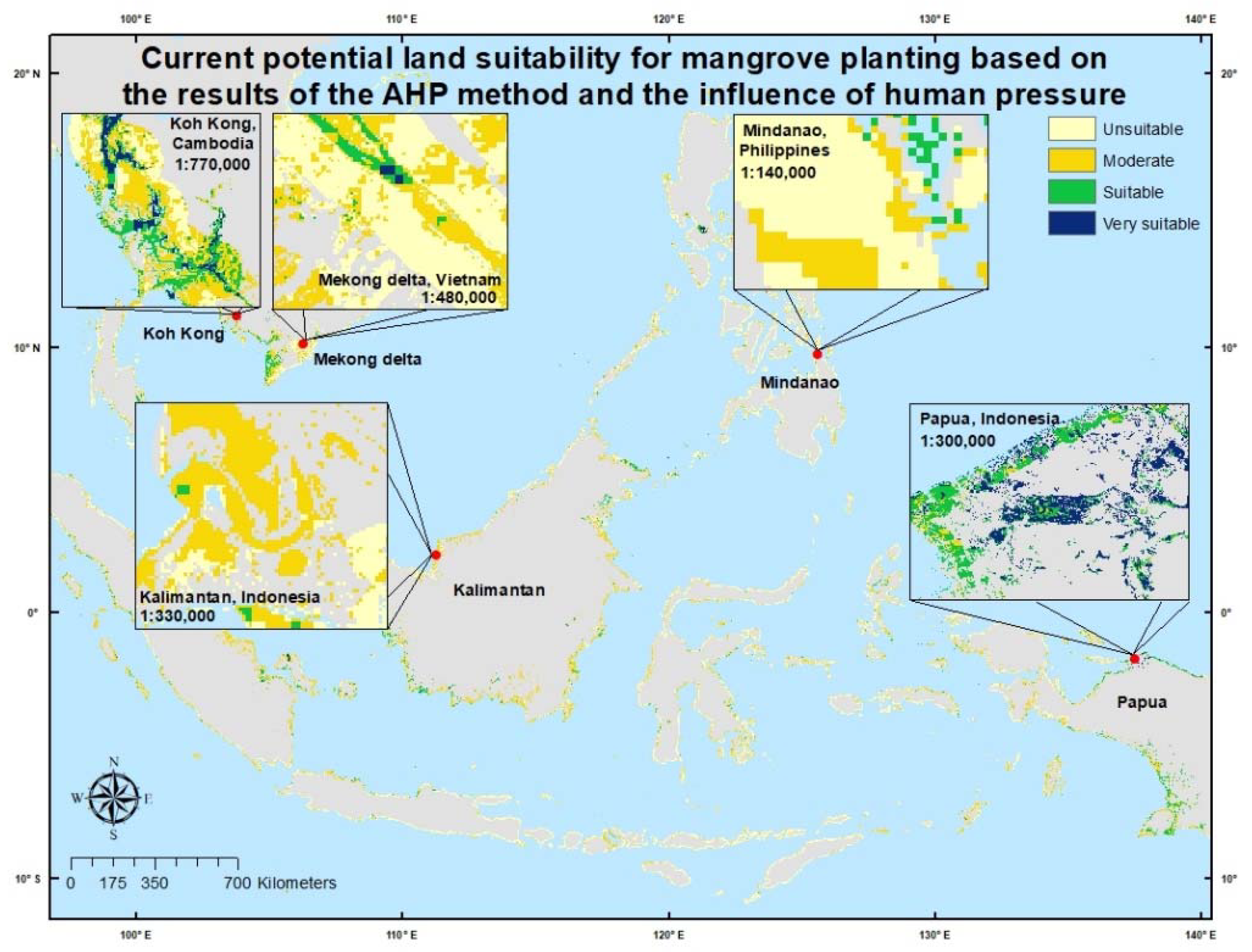
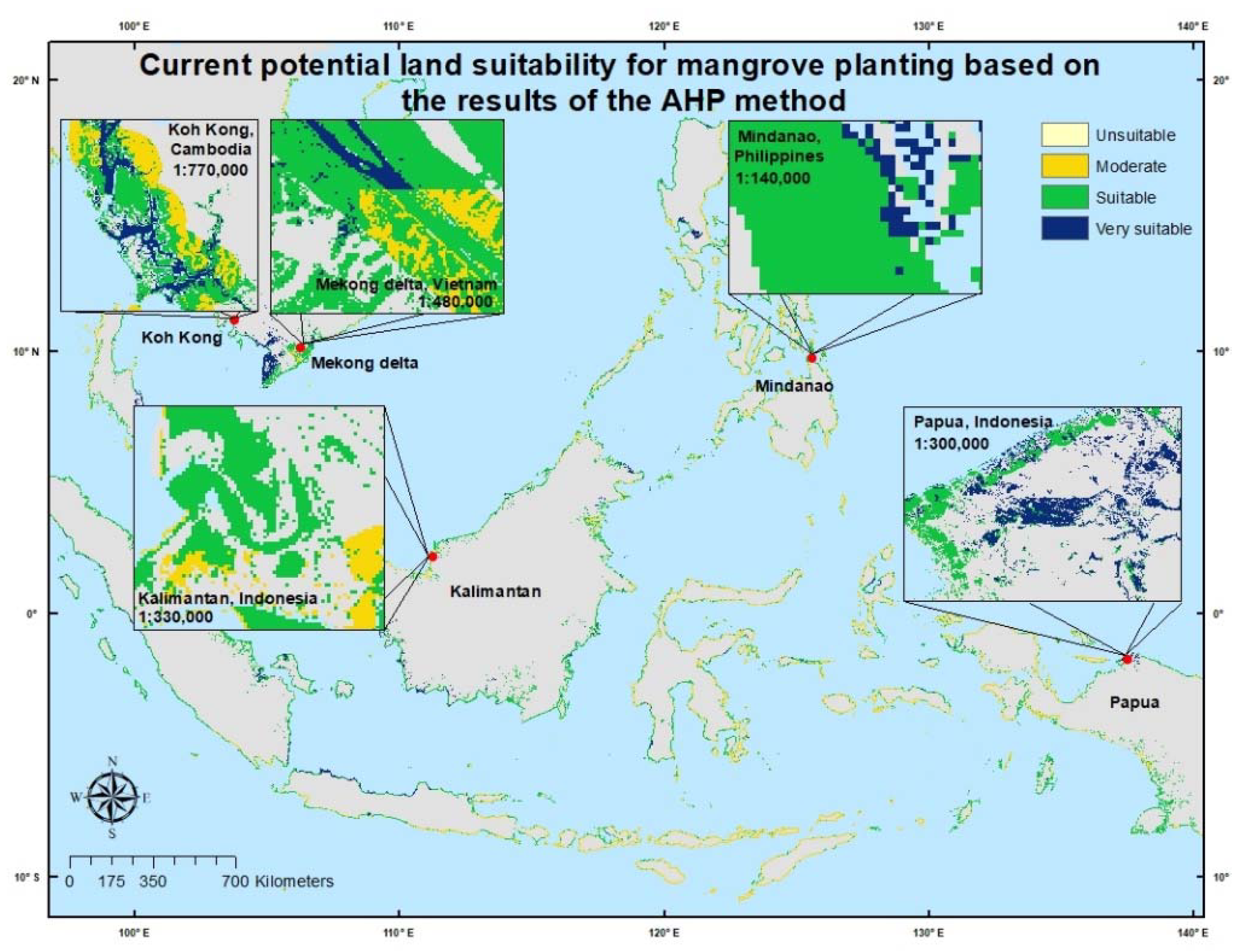
This study produced a land suitability map for mangrove planting in Southeast Asia, using the AHP technique, with a 250-m spatial resolution. The potential land suitability area were divided into three classes (very suitable, suitable, and moderate). The detailed results are shown for a selected region of Southeast Asia in Figure 2.

According to the land suitability map for mangrove planting that was generated using the AHP technique (Figure 2), approximately 3,960,000 ha of land have the potential to be very suitable for mangrove planting in Southeast Asia. The land that was classified as suitable and moderate for mangrove planting extended over 27,791,000 ha and 16,357,000 ha, respectively. The country that had the greatest potential was Indonesia, as it accounted for 57.38% of the total land area, including the very suitable and suitable categories (approximately 18,220,000 ha). Indonesia was followed by the Philippines, Malaysia, Vietnam, Thailand, and Myanmar with areas of 4,483,000 ha (14.12%), 2,725,000 ha (8.58%), 2,637,000 ha (8.31%), 1,679,000 ha (5.29%), and 1,530,000 ha (4.82%), respectively. The countries with the least land potential for mangrove planting were Cambodia (1.06%), Brunei Darussalam (0.29%), and Singapore (0.15%).

The inclusion of the human pressure parameters resulted in a significant change in the potential land area that could be suitable for mangrove planting in Southeast Asia. Based on the land suitability map for mangrove planting that was generated using the AHP technique combined with the human pressure parameters (Figure 3), there were approximately 398,000 ha of land suitable for mangrove planting in Southeast Asia. The land that was classified as suitable and moderate for mangrove planting was 4,771,000 ha and 20,123,000 ha, respectively.

Additionally, the order of the countries with the highest land potential for mangrove planting changed. The country with the largest potential land area was still Indonesia, which accounted for 67.34% of the total land area, including land in the very suitable and suitable categories, which was approximately 2,926,000 ha. Indonesia was followed by Vietnam, the Philippines, Thailand, Malaysia, and Cambodia with areas of 457,000 ha (10.52%), 287,000 ha (6.62%), 234,000 ha (5.38%), 182,000 ha (4.18%), and 143,000 ha (3.29%), respectively. The countries with the smallest area of land for mangroves planting were Myanmar (2.57%), Brunei Darussalam (0.09%), and Singapore (0.02%).

3.2. Current Potential Land Suitability for Mangrove Planting without the AHP Method

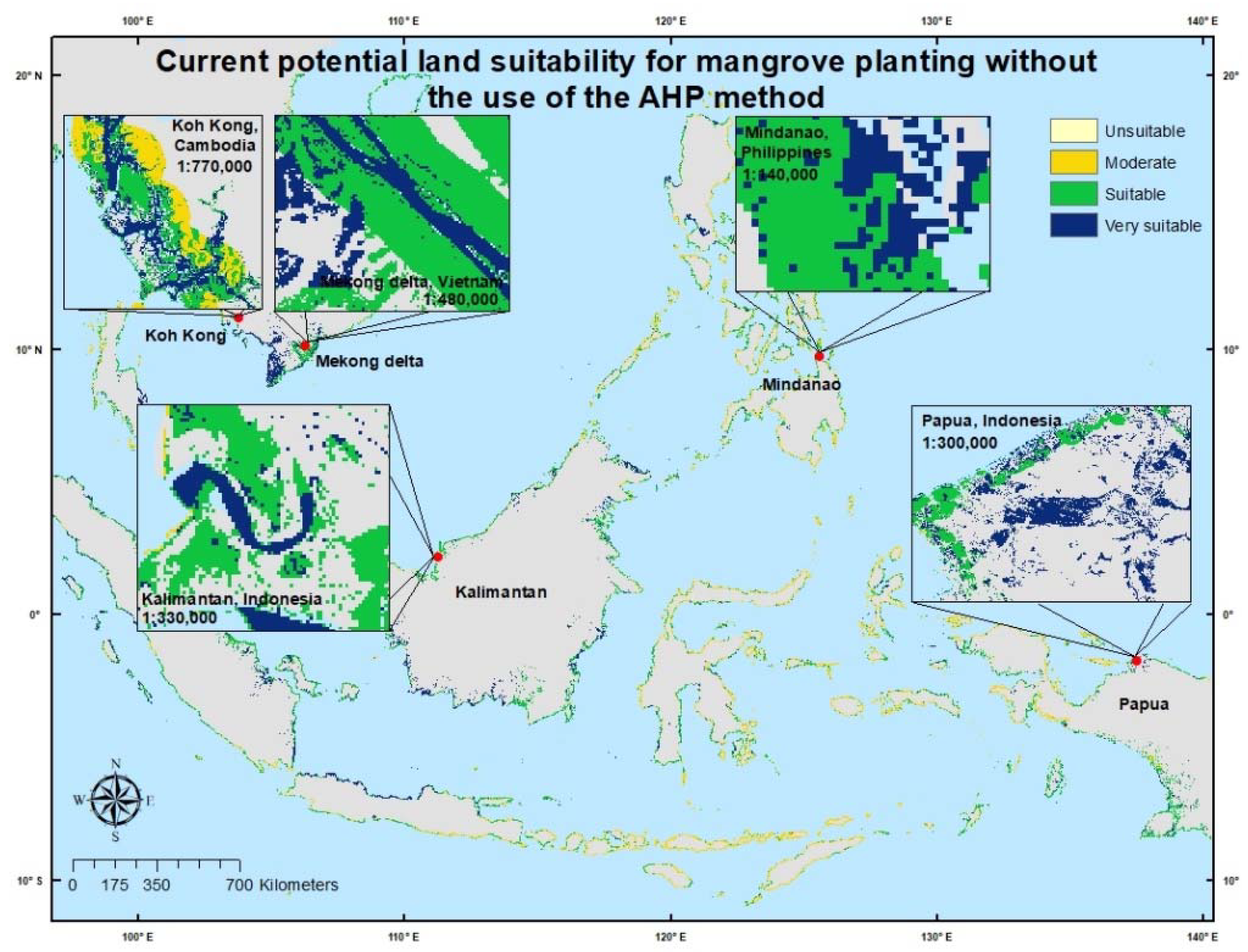
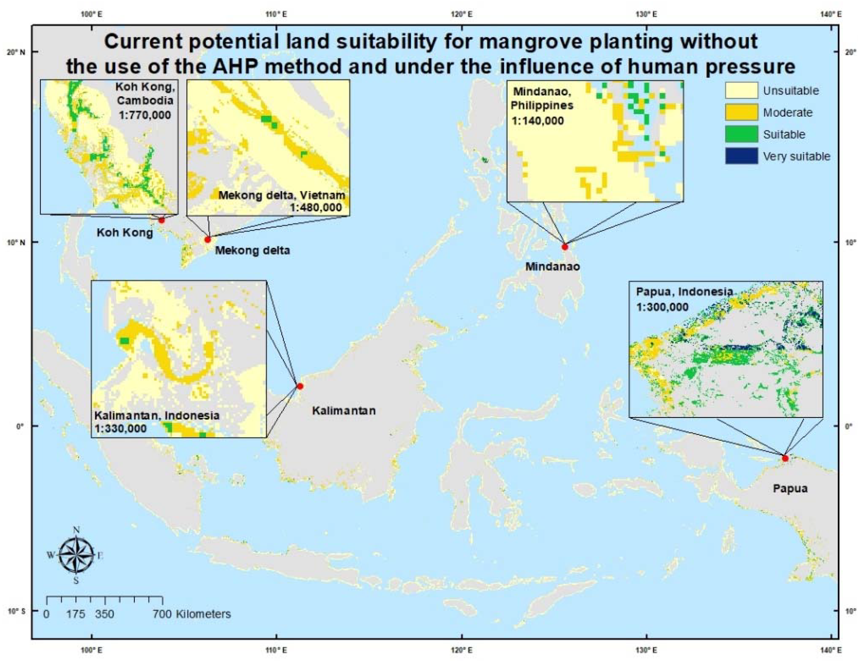
The differences in the potentially suitable land for mangrove planting with and without the use of the AHP technique (Figure 4 and Figure 5), which was used to determine the weight of each parameter, were compared. This comparative analysis aimed to determine the amount of influence the weighting produced by the AHP technique exerted on the potential suitability of the land for mangrove planting.

Based on the map of the land suitability potential without the use of the AHP technique (Figure 4), approximately 1,149,781 ha of land had the potential to be very suitable for planting mangroves in Southeast Asia. The land that was very suitable and suitable extended over 9,648,900 ha and 23,320,444 ha, respectively. The country with the greatest land potential for mangrove planting was Indonesia, as it accounted for 44.819% of the total land area, including very suitable and suitable categories of approximately 4,840,000 ha. Indonesia was followed by Myanmar, Vietnam, the Philippines, Thailand, and Malaysia with areas of 2,045,000 ha (18.940%), 1,331,000 ha (12.327%), 809,000 ha (7.494%), 781,000 ha (7.231%), and 753,000 ha (6.972%), respectively. Meanwhile, the countries with the least land potential for mangrove planting were Cambodia (1.956%), Brunei Darussalam (0.248%), and Singapore (0.014%).

In addition, this study mapped the potential land suitability for mangrove planting without using AHP, but considering the influence of the human pressure parameters (Figure 5). The resultant map of the land suitability potential showed that there appeared to be approximately 131,756 ha of potentially very suitable land in Southeast Asia. The very suitable and suitable land areas for mangrove planting were 939,231 ha and 6,988,350 ha, respectively. The country with the greatest land potential for mangrove planting was Indonesia, as it accounted for 59.326% of the total land area, including approximately 635,375 ha of land in the very suitable and suitable categories. The country with the second greatest land area suitable for mangrove planting was the Philippines with 118,806 ha (11.093%). The Philippines was followed by Vietnam, Thailand, Cambodia, and Malaysia with 104,063 ha (9.716%), 92,600 ha (8.646%), 55,025 ha (5.138%), and 36,488 ha (3.407%), respectively. The countries with the least land potential for mangrove planting were Myanmar (2.652%), Singapore (0.015%), and Brunei Darussalam (0.007%).

It is evident from the results that the analysis without the use of the AHP technique resulted in smaller areas of suitable and very suitable land (

Table 4. Areas of land classified as very suitable, suitable, and moderate in terms of planting mangroves in Southeast Asia both with and without the use of the analytic hierarchy process (AHP).

Weighting Technique	Country	Very Suitable (ha)	Suitable (ha)	Moderate (ha)
With AHP	Brunei Darussalam	0	4.050	26.388
	Indonesia	163.738	2762.350	12,741.319
	Cambodia	20.106	122.694	180.519
	Myanmar	1.006	110.638	1445.525
	Malaysia	769	180.975	1332.781
	Philippines	44.194	243.256	1752.450
	Singapore	100	694	11.138
	Thailand	60.538	173.075	662.563
	Vietnam	1.750	455.238	872.931
Without AHP	Brunei Darussalam	0	75	11.388
	Indonesia	52.688	582.688	4826.194
	Cambodia	4.488	50.538	152.625
	Myanmar	0	28.400	378.800
	Malaysia	13	36.475	428.294
	Philippines	18.206	100.600	339.219
	Singapore	0	156	1.100
	Thailand	56.263	36.338	270.825
	Vietnam	100	103.963	579.906

). This was because each parameter had a different weighed value, and these weight differences caused the higher-weighted parameters to be more important than the lower-weighted parameters. The results of the AHP technique indicated that the geomorphological parameters had the highest weight, accounting for approximately 38% of the total weight, which were followed by the hydrodynamic parameters and accounted for 32% of the total weight. The parameter with the smallest weight was the climate, which accounted for 30% of the total weight. These results showed that the geomorphological parameters were more important than the hydrodynamic and climate parameters. However, the weights of each of these parameters added up to the weights of each sub-parameter, which means that an area that has a large geomorphological parameter value may be no more suitable for mangrove planting than areas with high hydrodynamic values. This proves that the weight of each sub-parameter can be influential on the selection of potentially suitable lands for mangrove planting.

The results of the AHP technique analysis showed that the tidal inundation sub-parameter had the greatest weight when compared with the other sub-parameters. This was approximately four times the value of the smallest weight. The greater weight of this sub-parameter suggests that an area with tidal inundation classified in the very suitable, suitable, or moderate categories for mangrove planting will be preferred over areas in which other sub-parameters may have greater weights, even if they are classified as very suitable. In addition to the tidal inundation sub-parameter, the air temperature sub-parameter played an important role in the selection of potentially suitable land for mangrove planting. The air temperature sub-parameter ranked second in terms of importance after the tidal inundation sub-parameter and its weight was approximately three times that of the smallest weight. This suggests that the air temperature sub-parameter should be prioritized over the other three sub-parameters when selecting land that is potentially suitable for mangrove planting. The elevation and precipitation sub-parameters had the same weight and were considered equally important. However, when compared with the tidal inundation and air temperature, they were less important. The sub-parameter with the smallest weight, according to the results of the AHP technique, was slope.

The analysis of the potential land suitability for mangrove planting without the use of the AHP technique considered all parameters and sub-parameters as equally important in the selection of potentially suitable land for mangrove planting. The equalization of the parameter and sub-parameter weights gave a less accurate selection of the potentially suitable land than when the AHP method was used. Inaccurate land selection may result in the use of unsuitable land for mangrove planting or growth.

3.3. Land Suitability for Mangrove Planting Using the AHP Method and Climate Models

Two climate models were used to predict the potential land suitability for mangrove planting in Southeast Asia in 2050 and 2070. These were the CNRM-CM5.1 and the MIROC5.

3.3.1. Land Suitability for Mangrove Planting in 2050 and 2070 Using the CNRM-CM5.1 Model and the AHP Method

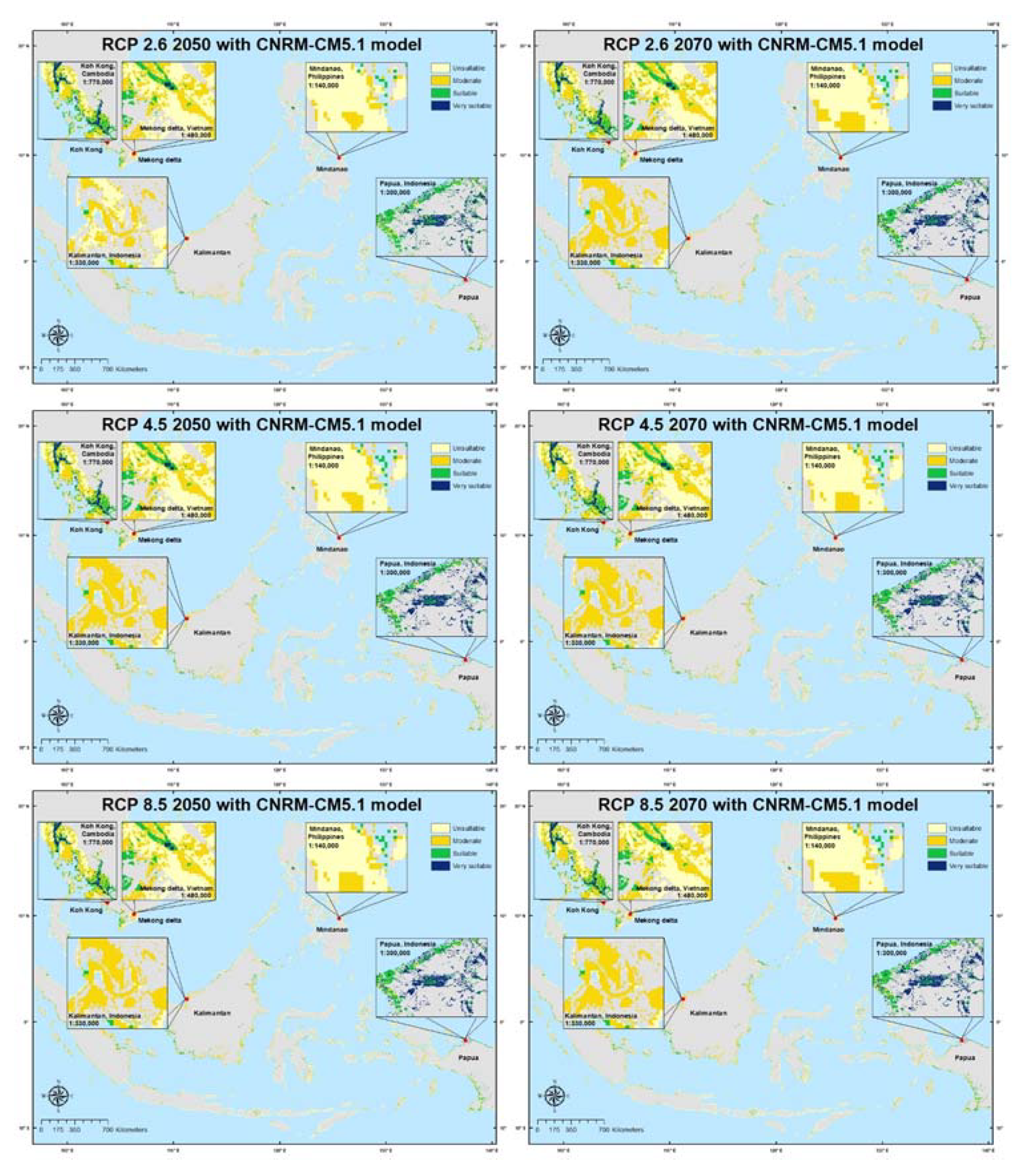
In the land suitability map for mangrove planting in 2050 constructed using the CNRM-CM5.1 model, the 2.6, 4.5, and 8.5 RCP scenarios were examined (Figure 6). There was a slight difference in the areas of the suitable land for mangrove planting among these three scenarios. RCP 8.5 resulted in the largest potential land area (324,125 ha), which was followed by RCP 4.5 (307,313 ha). RCP 2.6 resulted in the smallest suitable land area (264,906 ha). The difference in the land area of the very suitable category between RCP 8.5 and 2.6 was 59,219 ha.

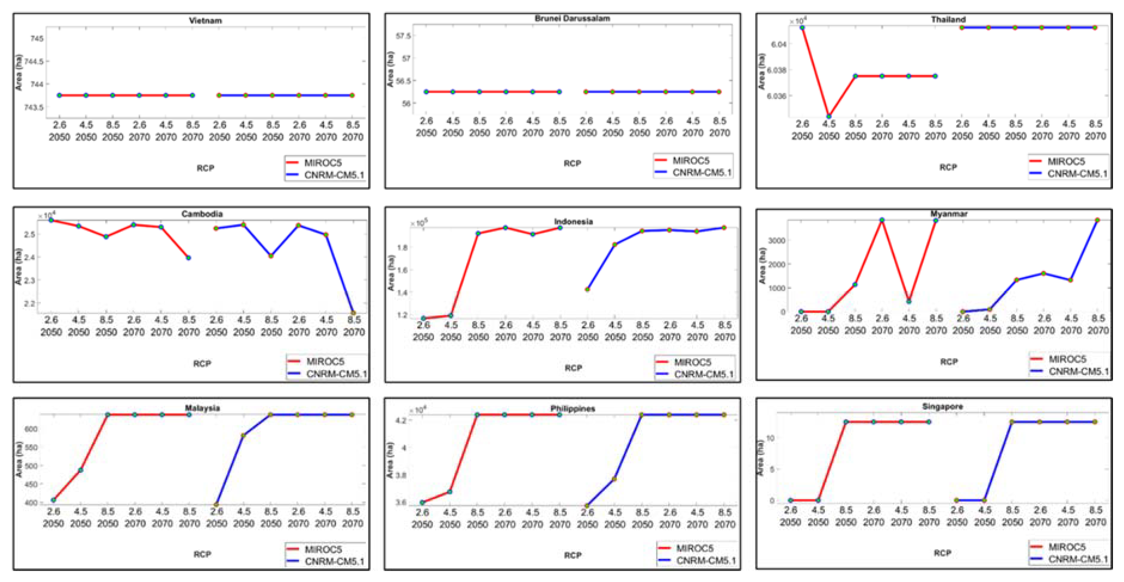
The results of the three RCPs were also different in terms of the area of the potential land area that was very suitable for mangrove planting in each country (Figure 7). Once again, Indonesia had the highest land suitability in all three RCPs. Additionally, Indonesia showed an increasing area of very suitable land from RCP 2.6 to 8.5 (52,181 ha). This increase was also observed for several other Southeast Asian countries, namely, the Philippines, Myanmar, and Malaysia, with increases of 6650 ha, 1331 ha, and 244 ha, respectively. However, Thailand, Vietnam, and Brunei Darussalam maintained the same area of very suitable potential land with all three RCPs. Singapore had the same potential land area with RCP 2.6 and 4.5, and it increased with RCP 8.5 by 13 ha. The suitable potential land area in Cambodia increased by 156 ha from RCP 2.6 to RCP 4.5. However, there was a drastic reduction of 1200 ha with RCP 8.5.

In contrast to 2050, for the three RCPs in 2070 (Figure 8 and Figure 9), the land area that was potentially very suitable for mangrove planting remained relatively similar for each RCP in most countries including Thailand, the Philippines, Vietnam, Malaysia, Brunei Darussalam, and Singapore. Indonesia experienced a decrease of 1219 ha in the potential land area from RCP 2.6 to RCP 4.5. However, the land area that was very suitable for mangrove planting in Indonesia increased by 3356 ha with RCP 8.5. Like Indonesia, the potential land area that was very suitable in Myanmar decreased by 281 ha from RCP 2.6 to RCP 4.5, and increased by 2519 ha with RCP 8.5. Conversely, in Cambodia, the very suitable potential land area decreased by 3813 ha from RCP 2.6 to RCP 8.5.

3.3.2. Potential Land Suitability for Mangrove Planting in 2050 and 2070 Using the MIROC5 Model and the AHP Method

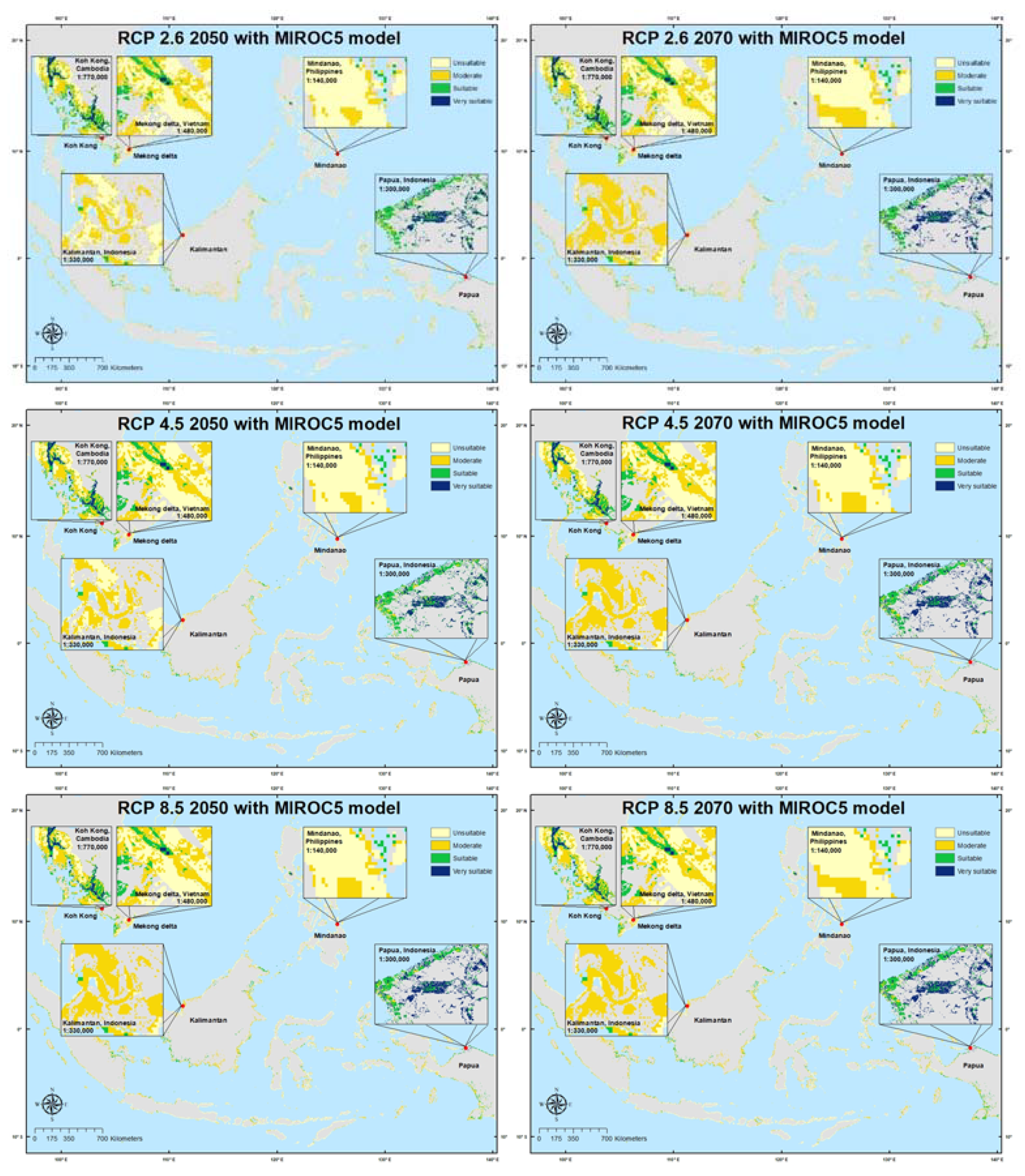
In the land suitability map constructed using the MIROC5 model 2050, the 2.6, 4.5, and 8.5 RCP scenarios were also assessed (Figure 8). There was a difference in the potential land area that was very suitable for mangrove planting among the three scenarios. The largest potential land area for mangrove planting in RCP 8.5 was 324,125 ha, whereas RCP 4.5 had a very suitable potential land area of 307,313 ha. RCP 2.6 had the least very suitable potential land area (264,906 ha). Therefore, the difference in the very suitable land area from RCP 8.5 to 2.6 was 82,838 ha.

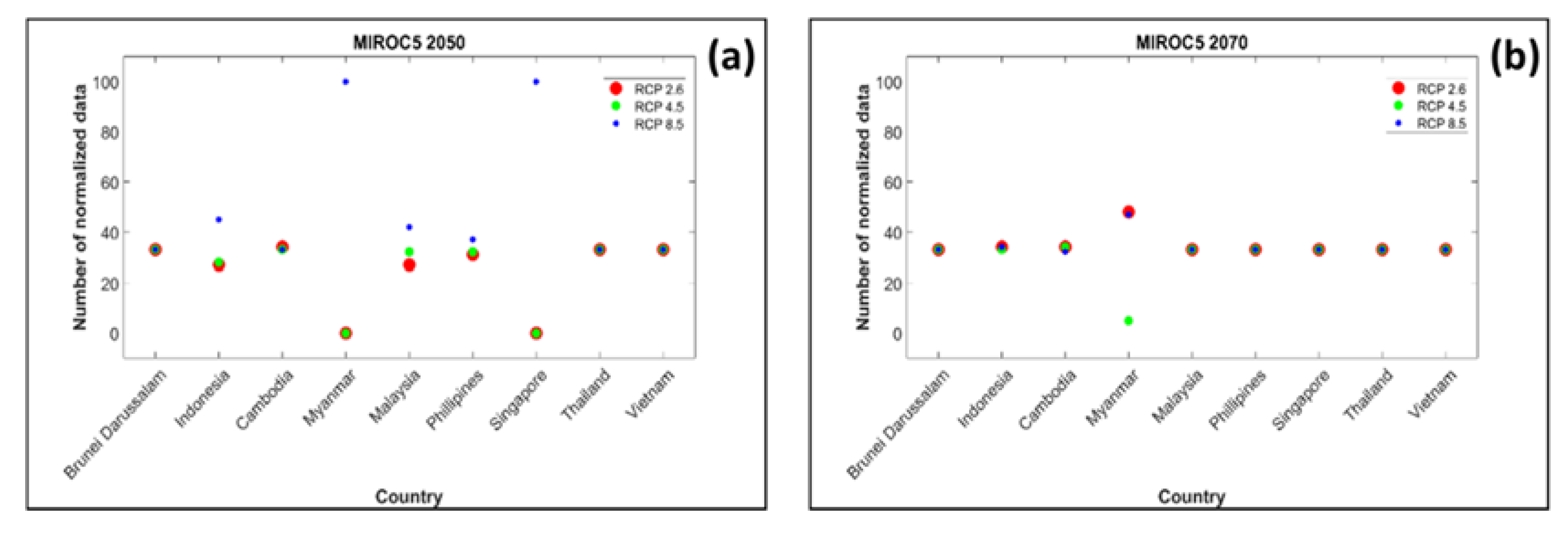
The three RCPs also differed in terms of the potential land area that was very suitable in each country (Figure 9). Indonesia had the largest potential land area suitable in all three RCPs, and it increased by 75,800 ha from RCP 2.6 to 8.5. An increase also occurred in several other Southeast Asian countries, namely, the Philippines, Myanmar, Malaysia, and Singapore. These experienced increases of 6413 ha, 1138 ha, 231 ha, and 13 ha, respectively. The area of the very suitable potential land in Vietnam and Brunei Darussalam remained the same in the three RCPs. The very suitable potential land area in Thailand decreased by 69 ha from RCP 2.6 to 4.5 and then increased by 3 ha with RCP 8.5. The suitable potential land area in Cambodia decreased by 719 ha from RCP 2.6 to RCP 8.5.

There were differences in the potentially suitable land area for mangrove planting (Figure 8). The largest area of potential very suitable land was found with RCP 2.6, which was 330,919 ha, whereas RCP 8.5 had the largest area of potential land area in the suitable category (329,381 ha). RCP 4.5 had the smallest land area in the very suitable category (321,506 ha) when compared with the other two RCPs. Therefore, there was a difference of 9413 ha in the very suitable land area from RCP 2.6 to RCP 4.5. Apart from the differences in the area of the very suitable potential land, the results of the three RCPs were relatively stable (Figure 8). The countries where the land area remained the same were Thailand, the Philippines, Vietnam, Malaysia, Brunei Darussalam, and Singapore. In contrast to the other countries, Indonesia experienced a drastic decrease of 5888 ha in a very suitable land area from RCP 2.6 to RCP 4.5. However, it experienced an increase of 5813 ha in the very suitable land area in RCP 8.5. Therefore, the decrease from RCP 2.6 to RCP 8.5 was 75 ha.

4. Discussion

4.1. Comparison of Our Results with Those of Other Studies

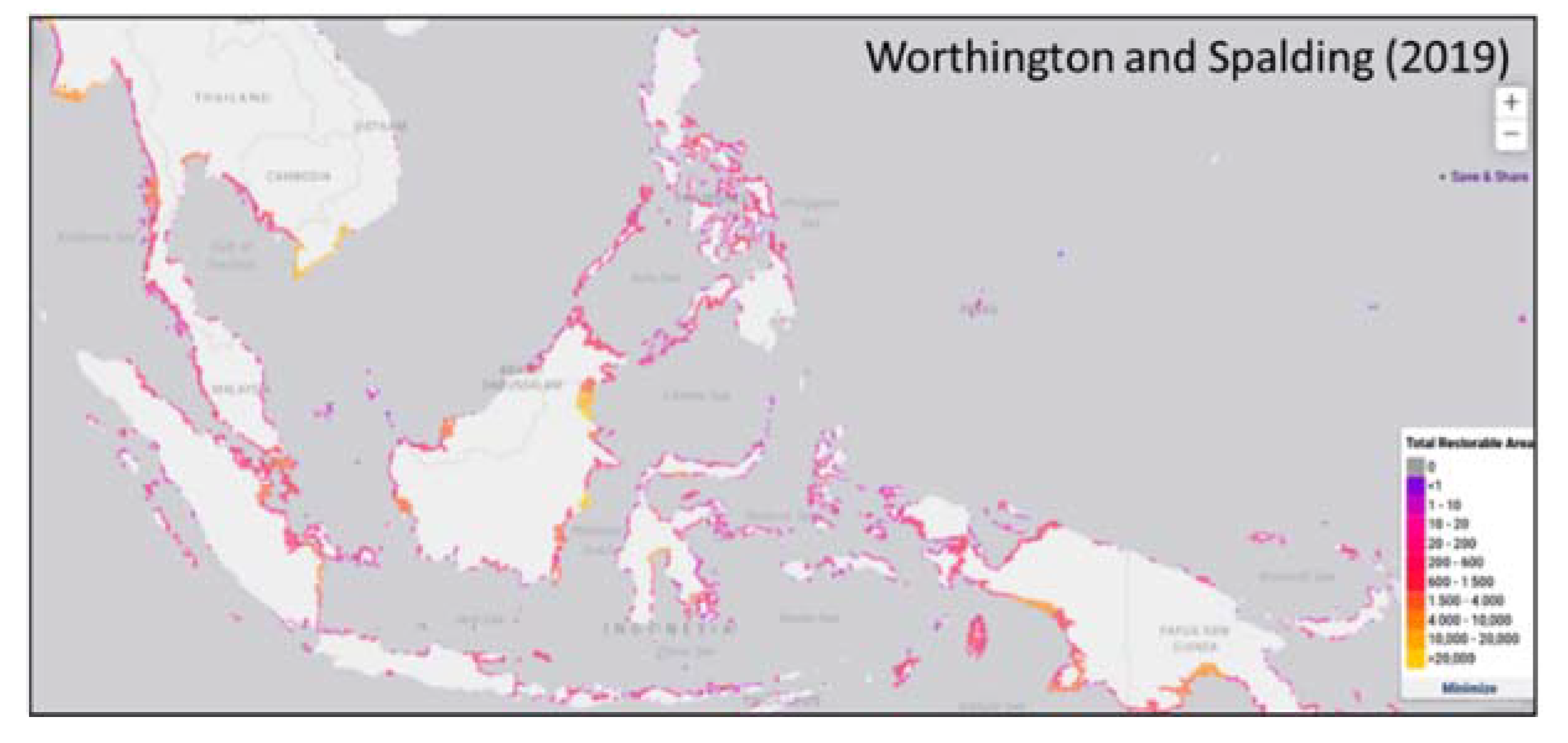
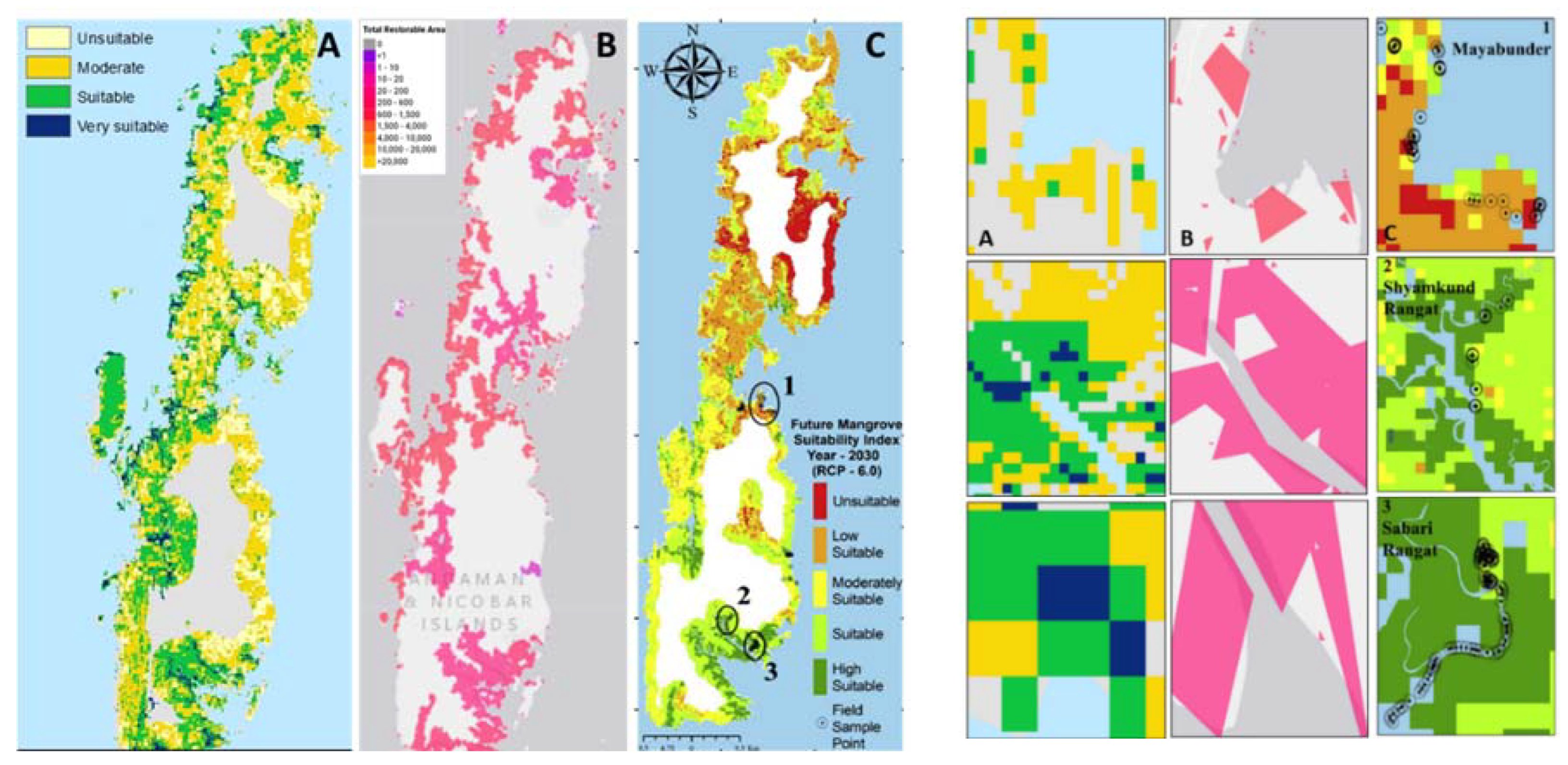
An additional feature of this study was the comparison of the results of the potential land suitability for mangroves that were obtained (with or without the use of the AHP method) with the results of Worthington and Spalding (2019, [102]) (Figure 10). The results of Worthington and Spalding (2019, [102]) showed that the total area with restoration potential was 303,708 ha. According to our results, the total area with the greatest potential (very suitable) to plant mangroves (with the use of the AHP technique) was 398,000 ha. Without the use of the AHP technique, this area was reduced to 131,756 ha.

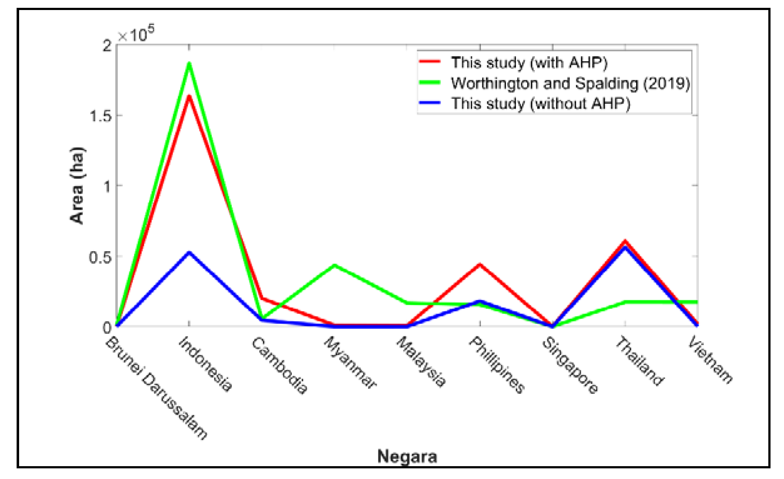
In addition, there were differences in the area of land that was determined to be very suitable for mangrove planting in each country (Figure 11). The sequence of countries obtained in this investigation that had the potential for mangrove planting is also different from the previously reported results of Worthington and Spalding (2019, [102]). In this investigation, the sequence of countries, in order from most suitable to least suitable, was Indonesia, Thailand, the Philippines, Cambodia, Vietnam, Myanmar, Malaysia, Singapore, and Brunei Darussalam. The corresponding sequence of the countries obtained without the use of the AHP technique was Thailand, Indonesia, the Philippines, Cambodia, Vietnam, Malaysia, Myanmar, Brunei Darussalam, and Singapore. According to the results of Worthington and Spalding (2019, [102]), the countries with the highest potentials for mangrove restoration were Indonesia, Myanmar, Thailand, Vietnam, Malaysia, the Philippines, Cambodia, Brunei Darussalam, and Singapore in order of potential. The differences were caused by the variations in the use of environmental parameters during data processing.

In addition, in this study, human pressure parameters were included. Therefore, an area that was classified as very suitable was selected not only because of the suitability of the environmental parameters but also because of the low human pressure parameter values. A high human pressure parameter value in a country was caused by high population growth and the GDP. In such a scenario, a larger land area will be required for the construction of socio-economic facilities. The results of this study showed that there were some countries with a smaller land area that were very suitable for mangrove planting when compared with other countries, which may have had larger mangrove areas.

In this study, all parameters were derived from remote sensing data and included environmental (hydrodynamic and geomorphology), climate, and human pressure parameters. However, the parameters used by Worthington and Spalding (2019, [102]) were tidal range, sea level rise, projected future sea level rise, sediment change, average size of mangrove loss, and proximity of the lost area to the remaining mangrove forest.

4.2. Comparison RCPs Scenario in Terms of the Potential Land Suitability for Mangrove Planting in the Future

In this study, two global climate models were used (namely, the CNRM-CM5.1 and the MIROC5) to predict the potential land suitability for mangrove planting in 2050 and 2070 with the RCP 2.6, 4.5, and 8.5. The different uses of the models created a number of different models of potential land suitability for mangrove planting. As shown in Figure 12, RCP 8.5 had the most suitable potential land area. This was due to the fact that its temperature increases were greater than those for the other RCPs (from 18.5 °C to 30.5 °C). In RCP 2.6 and RCP 4.5, the temperature increase was slightly lesser than that in RCP 8.5, from 18 °C to 29.9 °C, and 18.2 °C to 30.1 °C, respectively. Mangroves live and grow optimally at temperatures of 28 °C to 30 °C. This means that most Southeast Asian countries will have very suitable land area for the mangrove in RCP 8.5 in 2050. In contrast, mangrove land suitability predictions for 2070 showed that the majority of Southeast Asian countries maintained the same area across the three RCPs. This occurred because, in 2070, the lowest temperature was predicted to occur in RCP 4.5 (18.5–30.4 °C). RCP 8.5 was predicted to have the highest temperature in 2070, which ranged from 19.2 °C to 31.3 °C. On the other hand, RCP 2.6 had an intermediate temperature between RCP 4.5 and RCP 8.5 (18.5–30.5 °C). The temperature increase from RCP 2.6 to RCP 8.5 both in 2050 and 2070 means that the majority of Southeast Asian countries would have the same pattern in terms of very suitable land area for mangroves planting (Figure 13). Furthermore, the increased air temperature in 2050 and 2070 were not predicted across the temperature limits required for mangrove survival.

According to Duke et al. [45], mangroves will thrive with precipitation levels of 1400 to 3750 mm per year. According to the climate model data of MIROC5 and CNRM-CM5.1 in 2050 and 2070, the amount of precipitation per year in Southeast Asia will range from 0–1257 mm. For RCP 8.5 in 2070, the MIROC5 and CNRM-CM5.1 models had the highest precipitation values (12.574 and 988 mm per year, respectively). The increase in precipitation will also increase the number of areas suitable for planting mangroves in 2070, especially for RCP 8.5. This is consistent with the findings of Eslami-Andargoli et al. (2009, [39]), which increased precipitation, would result in the migration of mangrove forests in land and, consequently, increase the number of areas suitable for planting mangroves. However, the increasing number of inland mangrove areas with RCP 8.5 in 2070 can result in changes to the zonation of mangrove species [17,44,45]. An increase in precipitation could also reduce salinity [44,103,104]. Furthermore, each mangrove species has different hydrodynamic, geomorphological, and climatic criteria. Thus, if there is an increase in precipitation and temperature, some mangrove species would not survive and would eventually become extinct. At the same time, several surviving mangrove species would increase peat production due to decreased salinity and increased freshwater retention [105,106].

4.3. Uncertainties in Selecting Land Suitable for Mangrove Replanting

In this study, hydrodynamic, geomorphological, climatic, and socio-economic remote sensing data were used to produce maps of mangrove land suitability. The use of remote sensing data creates uncertainties related to the selection of the most suitable sites for mangrove planting and restoration. This is due to several reasons. First, the data used had different spatial resolutions. This can affect the interpretation of the suitability of the land for mangrove planting. Second, there were many parameters that affected the suitability of the land in terms of mangrove planting. However, most of these parameters have no available data. Some data were available, but their spatial resolutions were so coarse that they could not be used in this study. Owing to the limitations in the availability of these data, several other land suitability parameters were selected for this study. The parameters chosen had a higher level of importance in terms of the suitability of the land for mangrove planting than that of the other parameters. The AHP method was used to determine the importance level of each parameter. The determination of the level of importance for each parameter in the context of the AHP method resulted from expert judgment. However, some experts had conflicting opinions even though the results of the experts’ consistency assessments were consistent among the parameters. For example, expert A said that the tidal inundation parameter was the most influential parameter for selecting land suitable for mangrove planting, whereas expert B said that the most important parameter was slope. Both experts assigned values to each parameter consistently using the same rationale. This situation can also affect the land suitability results. Finally, the maps that predict the mangrove land suitability for 2050 and 2070 were created based on the assumption that hydrodynamic, geomorphological, and socio-economic parameters had fixed values based on the current situation even though this may not be the case. Furthermore, the sea-level rise parameters was not considered in this study. However, the sea-level rise is the most pertinent from global warming because it can change the duration of the swamps, their frequency, and salinity [46,107]. Therefore, the predicted results for 2050 and 2070 may be less accurate.

Table A3 explains that the CI value of 0.034 meant that the value of the relationship for each different variable had a fairly different similarity index and was also represented as having been sampled from our domain. Then, the sensitivity test was used to test which variables had changed with the first weight and the AHP weight. After the reduction, the differences in the tidal inundation (0.29), slope (0.19), elevation (0.23), air temperature (0.24), and precipitation (0.21) were obtained. In line with this, the slope parameter had the smallest difference in sensitivity with the total difference in sensitivity ${\sum }_{i=1}^5(S_i)=1.16$. It can then be interpreted that the use and employment of AHP here was appropriate, as proven by the Wilcoxon Test, which is a non-parametric version of the Student’s t-test with value (W = 25) and p-value = 0.007937 less than the significance level α = 5%. The true location shift is not equal to 0. The weight is the most important aspect in determining model performance, after which it is then necessary to pay attention to the parameters that are significant for model construction. If the weight increases, it takes longer time for a model to reach the maximum solution or convergence. Meanwhile, the Wilcoxon value also proved that the weight obtained was correct.

In addition, the results of this study were compared with several similar studies, namely, by Chakraborty et al. (2019, [56]) and Worthington and Spalding (2019, [102]) (Figure 14). The land suitability of the mangrove in the study by Worthington and Spalding [102] focused on areas lost since 1996. Factors such as tidal ranges, recent sea-level rises, projections of future sea-level rises, and recent sediment changes were added. The time since loss, mean size of patch lost, and proximity of the area lost to the remaining mangrove forests were analyzed using the Delphi method. Meanwhile, the land suitability of mangrove in another study [56] was made based on the climatic, geomorphic, edaphic, and floral conditions and the human interface parameters that were analyzed using the AHP method in the Northern and Central Andaman regions. Although there are some differences in the parameters and the methods used, the results of the mangrove land suitability maps produced by the three studies are very similar. For example, the results of the three studies in the Mayabunder area indicated that this location was relatively unsuitable for mangrove planting, whereas, in the Shyamkund Rangat area, all three studies indicated that most of the area was suitable for mangrove planting. Another example is that all three studies indicated that the Sahari Rangat area was very suitable for planting mangroves (Figure 14). This proves that some of the same parameters used in these three studies have a significant role in selecting suitable locations for mangroves. In addition, there are similarities in several locations suitable for mangrove planting.

4.4. Possible Future Directions

The results of this study can be applied in future research both in the environmental and the socio-economic sectors. One of the applications of this study could be to identify suitable land for planting mangroves in Southeast Asia. The reference map of the mangrove land suitability can help select areas that will be subjected to restoration before field surveys are conducted. However, to restore these areas, consideration should be paid to other mangrove land suitability parameters that were not included in this analysis. This will ultimately help minimize failures when planting mangroves. Part of this application includes an effort to implement sustainable development goals (SDGs) 13 and 14 regarding climate change and protecting the marine ecosystem [108].

A range of other important parameters should be included in future studies that are related to the suitability of land for mangrove planting. For example, determining mangrove species that are suitable to plant in areas subjected to either restoration or rehabilitation is of importance. Sea-level rises are also a restoration consideration in many areas. In addition, parameters for the future population growth models can also be added as barriers for the suitability of the land for future mangrove planting. Another research direction that could be followed is the examination of how much carbon will be absorbed if a number of areas are subjected to restoration. The findings of these studies will help elucidate how much greenhouse gas emissions will be reduced if mangrove restoration is carried out in a number of areas. This can support the implementation of greenhouse gas emission reduction targets in accordance with the Paris agreement [109]. The prediction of future mangrove suitability areas in 2050 and 2070 could also be improved by considering long-term changes in the anthropogenic and naturogenic impact [110], such as in agriculture areas [111,112], urban areas [113], and aquaculture practices [114]. These products could be integrated as one input data to make future analyses more realistic. Improving pixel resolution should also be considered to improve future analyses. Several techniques such as a spectral mixture model [115,116] and climate model interpolation [117,118] are key for producing high resolution images of mangrove replanting sites.

5. Conclusions

A map of the land suitable for mangrove planting in Southeast Asia was produced with a spatial resolution of 250 m, and was divided into four scenarios. The first scenario included the land suitability map for mangrove planting with the use of the AHP method. The second scenario included the AHP method and the influence of human pressure parameters. In the third scenario, all parameters were assumed to have the same level of importance and did not use the AHP model. Finally, in the fourth scenario, it was assumed that all parameters had the same level of importance, and the influence of the human pressure parameters was considered, but the AHP method was not used. The first and the second scenarios showed that approximately 3,960,000 ha and 398,000 ha of land, respectively, appeared to have the potential to be very suitable for mangrove planting. In scenarios three and four, approximately 1,149,781 ha and 131,756 ha of land, respectively, appeared to have the potential to be suitable for mangrove planting. All four scenarios showed that the country with the largest land area suitable for mangrove planting was Indonesia, which accounted for approximately 50%–60% of the total land included in the very suitable category in Southeast Asia. Moreover, this study presented a potential land suitability map for mangrove planting for 2050 and 2070 using two climate models (CNRM-CM5.1 and MIROC5) for each year. Each climate model had three RCP scenarios (2.6, 4.5, and 8.5). The results from both models showed that RCP 8.5 resulted in the largest land area suitable for mangrove planting in 2050 in the majority of the Southeast Asian countries. In 2070, almost all Southeast Asian countries had the same land area suitable for mangrove planting with all three RCPs. Future research could use feature selection in machine learning to overcome the shortcomings of the AHP method.

References

1. Baran, E. A review of quantified relationships between mangroves and coastal resources. Phuket Mar. Biol. Cent. Res. Bull. 1999, 62, 57–64. [Google Scholar]
2. Barbier, E.B.; Edward, B. Valuing the environmental as input: Review of applications to mangrove-fishery linkages. Ecol. Econ. 2000, 35, 47–61. [Google Scholar] [CrossRef]
3. Nagelkerken, L.; Blaber, S.J.M.; Bouillon, S.; Green, P.; Haywood, M.; Kirton, L.G.; Meynecke, J.-O.; Pawlik, J.; Penrose, H.M. The habitat function of mangroves for terrestrial and marine fauna: A review. Aqua Bot. 2008, 89, 155–185. [Google Scholar] [CrossRef] [Green Version]
4. Cannicci, S.; Burrows, D.; Fratini, S.; Smith III, T.J.; Offenberg, J.; Dahdouh-Guebas, F. Faunal impact on vegetation structure and ecosystem function in mangrove forests: A review. Aqua Bot. 2008, 89, 186–200. [Google Scholar] [CrossRef]
5. Barbier, E.B.; Hacker, S.D.; Kebbedy, C.; Loch, E.W.; Stier, A.C.; Silliman, B.R. The value of estuarine and coastal ecosystem services. Ecol. Soc. Am. 2011, 81, 169–193. [Google Scholar] [CrossRef]
6. Kathiresan, K.; Rajendran, N. Coastal mangrove forests mitigated tsunami. Estuar. Coast. Shelf Sci. 2005, 65, 601–606. [Google Scholar] [CrossRef]
7. Dahdouh-Guebas, F.; Jayatissa, L.P.; Nitto, D.D.; Bosire, J.O.; Seen, D.L.; Koedam, N. How effective were mangroves as a defence against the recent tsunami? Curr. Biol. 2005, 15, 12. [Google Scholar] [CrossRef] [Green Version]
8. Donato, D.C.; Kauffman, J.B.; Murdiyarso, D.; Kurnianto, S.; Stidham, M.; Kanninen, M. Mangroves among the most carbon-rich forests in the tropics. Nat. Geosci. 2011, 4, 293–297. [Google Scholar] [CrossRef]
9. Robertson, A.I.; Duke, N.C. Mangrove fish-communities in tropical Queensland, Australia: Spatial and temporal patterns in densities, biomass and community structure. Mar. Biol. 1990, 104, 369–379. [Google Scholar] [CrossRef]
10. Paillon, C.; Wantiez, L.; Kulbicki, M.; Labonne, M.; Vigliola, L. Extent of mangrove nursery habitats determines the geographic distribution of coral reef fish in a South-Pacific Archipelago. PLoS ONE 2014, 9, e105158. [Google Scholar] [CrossRef]
11. Mcleod, E.; Chmura, G.L.; Bouillon, S.; Salm, R.; Björk, M.; Duarte, C.M.; Lovelock, C.E.; Schlesinger, W.H.; Silliman, B.R. A blueprint for blue carbon: Toward an improved understanding of the role of vegetated coastal habitats in sequestering CO2. Front. Ecol. Environ. 2011, 9, 552–560. [Google Scholar] [CrossRef] [Green Version]
12. Spalding, M.D.; Blasco, F.; Field, C.D. World Mangrove Atlas, 3rd ed.; The International Society for Mangrove Ecosystems: Okinawa, Japan, 1997; 178p. [Google Scholar]
13. Giri, C.; Ochieng, E.; Tieszen, L.L.; Zhu, Z.; Singh, A.; Loveland, T.; Masek, J.; Duke, N. Status and distribution of mangrove forests of the world using earth observation satellite data. Glob. Ecol. Biogeogr. 2011, 20, 154–159. [Google Scholar] [CrossRef]
14. Food and Agriculture Organization (FAO) of the United Nations. The world’s mangroves 1980–2005. FAO For. Pap. 2007, 153, 18–77. [Google Scholar]
15. Richards, D.R.; Friess, D.A. Rates and drives of mangrove deforestation in Southeast Asia, 2000–2012. Proc. Natl. Acad. Sci. USA 2016, 113, 344–349. [Google Scholar] [CrossRef] [PubMed] [Green Version]
16. Polidoro, B.A.; Carpenter, K.E.; Collins, L.; Duke, N.C.; Ellison, A.M.; Ellison, J.C.; Ellison, J.C.; Farnsworth, E.J.; Fernando, E.S.; Kathiresan, K.; et al. The loss of species: Mangrove extinction risk and geographic areas of global concern. PLoS ONE 2010, 5, e10095. [Google Scholar] [CrossRef]
17. Gilman, E.L.; Ellison, J.; Duke, N.C.; Field, C. Threats to mangroves from climate change and adaptation options: A review. Aqua Bot. 2008, 89, 237–250. [Google Scholar] [CrossRef]
18. Alongi, D.M. The impact of climate change on mangrove forests. Curr. Clim. Chang. Rep. 2015, 1, 30–39. [Google Scholar] [CrossRef]
19. Ward, R.D.; Friess, D.A.; Day, R.H.; Mackenzie, R.A. Impacts of climate change on mangrove ecosystems: A region by region overview. Ecosyst. Health Sustain. 2016, 2, 1–25. [Google Scholar] [CrossRef] [Green Version]
20. Riascos, J.M.; Cantera, J.R.; Blanco-Libreros, J.F. Growth and mortality of mangrove seedlings in the wettest neotropical mangrove forests during ENSO: Implications for vulnerability to climate change. Aquat. Bot. 2018, 147, 34–42. [Google Scholar] [CrossRef]
21. Aburto-oropeza, O.; Ezcurra, E.; Danemann, G.; Valdez, V.; Murray, J.; Sala, E. Mangroves in the Gulf of California increase fishery yields. Proc. Natl. Acad. Sci. USA 2007, 105, 10456–10459. [Google Scholar] [CrossRef] [Green Version]
22. Andradi-Brown, D.A.; Howe, C.; Mace, G.M.; Knight, A.T. Do mangrove forest restoration or rehabilitation activities return biodiversity to pre-impact levels? Environ. Evid. 2013, 2, 1–8. [Google Scholar] [CrossRef] [Green Version]
23. Elster, C. Reasons for reforestation success and failure with three mangrove species in Columbia. For. Ecol. Manag. 2000, 131, 201–214. [Google Scholar] [CrossRef]
24. Lewis, R.R., III. Ecological engineering for successful management and restoration of mangrove forests. Ecol. Eng. 2005, 24, 403–418. [Google Scholar] [CrossRef]
25. Primavera, J.H.; Esteban, J.M.A. A review of mangrove rehabilitation in the Philippines: Successes, failures and future prospects. Wetl. Ecol. Manag. 2008, 16, 345–358. [Google Scholar] [CrossRef]
26. Samson, M.S.; Rollon, R.N. Growth performance of planted mangrove in the Philippines: Revisiting forest management strategies. AMBIO 2008, 37, 234–240. [Google Scholar] [CrossRef]
27. Zaldívar-Jiménez, M.A.; Herrera-Silveira, J.A.; Teutli-Hernández, C.; Comín, F.A.; Andrade, J.L.; Molina, C.C.; Ceballos, R.P. Conceptual framework for mangrove restoration in the Yucatán Peninsula. Ecol. Restor. 2010, 28, 333–342. [Google Scholar] [CrossRef] [Green Version]
28. Winterwerp, J.C.; Erftemeijer, P.L.A.; Suryadiputra, N.; van Eijk, P.; Zhang, L. Defining eco-morphodynamic requirements for rehabilitating eroding mangrove-mud coasts. Wetlands 2013, 33, 515–526. [Google Scholar] [CrossRef]
29. Brown, B.; Fadillah, R.; Nurdin, Y.; Soulsby, I.; Ahmad, R. Community based ecological mangrove rehabilitation (CBEMR) in Indonesia. Surv. Perspect. Integr. Environ. Soc. 2014, 7, 1–11. [Google Scholar]
30. Kodikara, K.A.S.; Mukherjee, N.; Jayatissa, L.P.; Dahdouh-Guebas, F.; Koedam, N. Have mangrove restoration projects worked? An in-depth study in Sri Lanka. Restor. Ecol. 2017, 25, 705–716. [Google Scholar] [CrossRef]
31. Earlie, C.; Masselink, G.; Russell, P. The role of beach morphology on coastal cliff erosion under extreme waves. Earth Surf. Process Landf. 2018, 43, 1213–1228. [Google Scholar] [CrossRef] [Green Version]
32. Peng, Y.S.; Zhou, Y.W.; Hou, Y.W.; Chen, G.Z. The restoration of mangrove wetlands: A review. Acta Ecol. Sin. 2008, 28, 786–797. [Google Scholar]
33. Maslin, M.; Austin, P. Climate models at their limit? Nature 2012, 486, 183–184. [Google Scholar] [CrossRef] [PubMed]
34. Intergovermental Panel on Climate Change (IPCC). Climate change 2013: The physical science basis. In Contribution of Working Group I to the Fifth Assessment Report of the Intergovermental Panel on Climate Change; Cambridge University Press: Cambridge, UK; New York, NY, USA, 2013; 1535p. [Google Scholar]
35. Schewe, J.; Levermann, A. A statistically predictive model for future monsoon failure in India. Environ. Res. Lett. 2012, 7, 1–9. [Google Scholar] [CrossRef] [Green Version]
36. Ashfaq, M.; Shi, Y.; Tung, W.; Trapp, R.J.; Gao, X.; Pal, J.S.; Diffenbaugh, N.S. Suppression of South Asian summer monsoon precipitation in the 21st century. Geophys. Res. Lett. 2009, 26, L01704. [Google Scholar] [CrossRef] [Green Version]
37. Loo, Y.Y.; Billa, L.; Singh, A. Effect of climate change on seasonal monsoon in Asia and its impact on the variability of monsoon rainfall in Southeast Asia. Geosci. Front. 2015, 6, 817–823. [Google Scholar] [CrossRef] [Green Version]
38. Fischer, E.M.; Knutti, R. Detection of spatially aggregated changes in temperature and precipitation extremes. Geophys. Res. Lett. 2014, 41, 547–554. [Google Scholar] [CrossRef]
39. Eslami-Andargoli, L.; Dale, P.; Sipe, N.; Chaseling, J. Mangrove expansion and rainfall patterns in Moreton Bay, Southeast Queensland, Australia. Estuar. Coast. Shelf Sci. 2009, 85, 292–298. [Google Scholar] [CrossRef] [Green Version]
40. Gilman, E.; Ellison, J. Efficacy of alternative low-cost approach to mangrove restoration, American Samoa. Estuaries Coasts 2007, 30, 641–651. [Google Scholar] [CrossRef]
41. Bathiany, S.; Dakos, V.; Scheffer, M.; Lenton, T.M. Climate models predict increasing temperature variability in poor countries. Sci. Adv. 2018, 4, 1–10. [Google Scholar] [CrossRef] [Green Version]
42. Coumou, D.; Rahmstorf, S. A decade of seather extremes. Nat. Clim. Chang. 2012, 2, 491–496. [Google Scholar] [CrossRef]
43. Arnell, N.W. Climate change and global water resources: SRES emissions and socio-economic scenarios. Glob. Environ. Chang. 2004, 14, 31–51. [Google Scholar] [CrossRef]
44. Field, C. Impacts of expected climate change on mangroves. Hydrobiologia 1995, 295, 75–81. [Google Scholar] [CrossRef]
45. Duke, N.C.; Ball, M.C.; Ellison, J.C. Factors influencing biodiversity and distributional gradients in mangrove. Glob. Ecol. Biogeogr. 1998, 7, 27–47. [Google Scholar] [CrossRef] [Green Version]
46. Smith, T.J., III; Duke, N.C. Physical determinants of inter-estuary variation in mangrove species richness around the tropical coastline of Australia. J. Biogeogr. 1987, 14, 9–19. [Google Scholar] [CrossRef]
47. Ball, M.C.; Sobrado, M.A. Ecophysiology of mangroves: Challenges in linking physiological processes with patterns in forest structure. In Advances in Plant Physiological Ecology; Press, M.C., Scholes, J.D., Barker, M.G., Eds.; Blackwell Science: Oxford, UK, 2002; pp. 331–346. [Google Scholar]
48. Small, C.; Nicholls, R.J. A global analysis of human settlement in coastal zones. J. Coast. Res. 2003, 19, 584–599. [Google Scholar]
49. Balk, D.; Montgomery, M.R.; McGranahan, G.; Kim, D.; Mara, V.; Todd, M.; Buettner, T.; Dorelien, A. Mapping urban settlements and the risks of climate change in Africa, Asia and South America. Popul. Dyn. Clim. Chang. 2009, 80, 103. [Google Scholar]
50. McGranahan, G.; Balk, D.; Anderson, B. The rising tide: Assessing the risks of climate change and human settlements in low elevation coastal zones. Environ. Urban. 2007, 19, 17–37. [Google Scholar] [CrossRef]
51. Smith, K. We are sevel billion. Nat. Clim. Chang. 2011, 1, 331–335. [Google Scholar] [CrossRef]
52. Vo, Q.T.; Oppelt, N.; Leinenkugel, P.; Kuenzer, C. Remote sensing in mapping mangrove ecosystems-an object-based approach. Remote Sens. 2013, 5, 183–201. [Google Scholar] [CrossRef] [Green Version]
53. Zhen, J.; Liao, J.; Shen, G. Mapping mangrove forests of Dongzhaigang nature reserve in China using Landsat 8 and Radarsat-2 polimetric SAR data. Sensors 2018, 18, 4012. [Google Scholar] [CrossRef] [Green Version]
54. Liu, K.; Li, X.; Shi, X.; Wang, S. Monitoring mangrove forest changes using remote sensing and GIS data with decision-tree learning. Wetlands 2008, 28, 336–346. [Google Scholar] [CrossRef]
55. Fauzi, A.; Sakti, A.; Yayusman, L.; Harto, A.; Prasetyo, L.; Irawan, B.; Kamal, M.; Wikantika, K. Contextualizing mangrove forest deforestation in Southeast Asia using environmental and socio-economic data product. Forests 2019, 10, 952. [Google Scholar] [CrossRef] [Green Version]
56. Chakraborty, S.; Sahoo, S.; Majumdar, D.; Saha, S.; Roy, S. Future mangrove suitability assessment of Andaman to strengthen sustainable development. J. Clean. Prod. 2019, 234, 597–614. [Google Scholar] [CrossRef]
57. Monsef, H.A.; Hassan, M.A.A.; Shata, S. Using spatial data analysis for delineating existing mangroves stands and siting suitable locations for mangroves plantation. Comput. Electron. Agric. 2017, 141, 310–326. [Google Scholar] [CrossRef]
58. Wang, F. The use of artificial neural networks im a geographical information system for agricultural land-suitability assessment. Environ. Plan. 1994, 26, 265–284. [Google Scholar] [CrossRef]
59. Bagherzadeh, A.; Ghadiri, E.; Darban, A.R.S.; Gholizadeh, A. Land suitability modeling by parametric-based neural networks and fuzzy methods for soybean production in a semi-arid region. Modeling Earth Syst. Environ. 2016, 2, 1–11. [Google Scholar] [CrossRef] [Green Version]
60. Bojórquez-Tapia, L.A.; Diaz-Mondragón, S.; Ezcurra, E. GIS-based approach for participatory decision making and land suitability assessment. Int. J. Geogr. Inf. Sci. 2001, 15, 129–151. [Google Scholar] [CrossRef]
61. Joerin, F.; Thériault, M.; Musy, A. Using GIS and outranking multicriteria analysis for land-use suitability assessment. Int. J. Geogr. Inf. Sci. 2001, 15, 153–174. [Google Scholar] [CrossRef]
62. Kalogirou, S. Expert systems and GIS: An application of land suitability evaluation. Comput. Environ. Urban Syst. 2002, 26, 89–112. [Google Scholar] [CrossRef]
63. Shalaby, A.; Ouma, Y.O.; Tateishi, R. Land suitability assessment for perennial crops using remote sensing and geographic information system: A case study in northwestern Egypt. Arch. Agron. Soil Sci. 2006, 52, 243–261. [Google Scholar] [CrossRef]
64. Foshtomi, M.D.; Norouzi, M.; Rezaei, M.; Akef, M.; Akbarzadeh, A. Qualitative and economic land suitability evaluation for tea (Camellia sinesis L.). J. Biol. Environ. Sci. 2011, 5, 135–146. [Google Scholar]
65. Olayeye, A.O.; Akinbola, G.E.; Marake, V.M.; Molete, S.F.; Mapheshoane, B. Soil in suitability evaluation for irrigated lowland rice culture in Southwestern Nigeria: Management implication for sustainability. Commun. Soil Sci. Plant Anal. 2008, 39, 2920–2938. [Google Scholar] [CrossRef]
66. Chandio, I.A.; Matori, A.N.; Yusof, K.; Talpur, M.A.H.; Aminu, M. GIS-basedland suitability analysis of sustainable hillside development. Procedia Eng. 2014, 77, 87–94. [Google Scholar] [CrossRef] [Green Version]
67. Bandyopadhyay, S.; Jaiswal, R.K.; Hegde, V.S.; Jayaraman, V. Assessment of land suitability potentials for agriculture using a remote sensing and GIS based approach. Int. J. Remote Sens. 2009, 30, 879–895. [Google Scholar] [CrossRef]
68. Cengiz, T.; Akbulak, C. Application of analytical hierarchy process and geographic information systems in land-use suitability evaluation: A case study of Dȕmrek village (Canakkale, Turkey). Int. J. Sustain. Dev. World Ecol. 2009, 16, 286–294. [Google Scholar] [CrossRef]
69. Jafari, S.; Zaredar, N. Land suitability analysis using multi attributr decision making approach. Int. J. Environ. Sci. Dev. 2010, 1, 441–445. [Google Scholar] [CrossRef]
70. Chandio, I.A.; Matori, A.N.; Lawal, D.U.; Sabri, S. GIS- based land suitability analysis using AHP for public parks planning in Larkana City. Mod. Appl. Sci. 2011, 5, 177–189. [Google Scholar] [CrossRef] [Green Version]
71. Feizizadeh, B.; Blaschke, T. Land suitability analysis for Tabriz Country, Iran: A multi-criteria evaluation approach using GIS. J. Environ. Plan. Manag. 2012, 56, 1–23. [Google Scholar] [CrossRef]
72. Akinci, H.; Özalp, A.Y.; Turgut, B. Agricultural land use suitability analysis using GIS and AHP technique. Comput. Electron. Agric. 2013, 97, 71–82. [Google Scholar] [CrossRef]
73. García, J.L.; Alvarado, A.; Blanco, J.; Jiménez, E.; Maldonado, A.A.; Cortés, G. Multi-attribute evaluation and selection of sites for agricultural product warehouses based on an analytic hierarchy process. Comput. Electron. Agric. 2014, 100, 60–69. [Google Scholar] [CrossRef] [Green Version]
74. Yi, X.; Wang, L. Land suitability assessment on a watershed of Loess Plateau using the analytic hierarchy process. PLoS ONE 2013, 8, e69498. [Google Scholar] [CrossRef]
75. Parry, J.A.; Ganaie, S.A.; Bhat, M.S. GIS based land suitability analysis using AHP model for urban services planning in Srinagar and Jammu urban centers of J&K, India. J. Urban Manag. 2018, 7, 46–56. [Google Scholar]
76. Arulbalaji, P.; Padmalal, D.; Sreelash, K. GIS and AHP techniques based delineation of groundwater potential zones: A case study from Southern Western Ghats, India. Sci. Data 2019, 9, 1–17. [Google Scholar] [CrossRef] [PubMed]
77. Chen, Z.; Chen, T.; Qu, Z.; Yang, Z.; Ji, X.; Zhou, Y.; Zhang, H. Use of evidential reasoning and AHP to assess regional industrial safety. PLoS ONE 2018, 13, 1–21. [Google Scholar] [CrossRef] [PubMed] [Green Version]
78. Papathoma-Köhle, M.; Schlögl, M.; Fuchs, S. Vulnerability indicators for natural hazards: An innovative selection and weighting approach. Sci. Rep. 2019, 9, 1–14. [Google Scholar] [CrossRef] [PubMed]
79. Saaty, R.M. The analytic hierarchy process-what it is and how it is used. Math. Model. 1987, 9, 161–176. [Google Scholar] [CrossRef] [Green Version]
80. Egbert, G.D.; Bennett, A.F. TOPEX/POSEIDON tides estimated using a global inverse model. J. Geophys. Res. 1994, 99, 24821–24852. [Google Scholar] [CrossRef] [Green Version]
81. Egbert, G.D.; Erofeeva, S.Y. Efficient inverse modeling of barotropic ocean tides. Am. Meteorol. Soc. 2002, 19, 183–203. [Google Scholar] [CrossRef] [Green Version]
82. Yamazaki, D.; Ikeshima, D.; Tawatari, R.; Yamaguchi, T.; O’Loughlin, F.; Nael, C.J.; Sampson, C.C.; Kanae, S.; Bates, P.D. A high-accuracy map of global terrain elevations. Geophys. Res. Lett. 2017, 44, 5844–5853. [Google Scholar] [CrossRef] [Green Version]
83. Janowiak, J.E.; Joyce, R.J.; Yarosh, Y. A real-time global half-hourly pixel-resolution infrared dataset and its applications. Bull. Am. Meteorol. Soc. 2001, 82, 205–217. [Google Scholar] [CrossRef] [Green Version]
84. Saha, S.; Moorthi, S.; Pan, H.L.; Wu, X.; Wang, J.; Nadiga, S.; Tripp, P.; Kistler, R.; Woollen, J.; Behringer, D.; et al. The NCEP climate forecast system reanalysis. Am. Meteorol. Soc. 2010, 91, 1015–1057. [Google Scholar] [CrossRef]
85. Funk, C.; Peterson, P.; Landsfeld, M.; Pedreros, D.; Verdin, J.; Shukla, S.; Husak, G.; Rowland, J.; Harrison, L.; Hoell, A.; et al. The climate hazards infrared precipitation with stations-a new environmental record for monitoring extremes. Sci. Data 2015, 2, 1–21. [Google Scholar] [CrossRef] [PubMed] [Green Version]
86. Di Gregorio, A. UN Land Cover Classification System (LCCS)-Classification Concepts and User Manual for Software Version 2; Food Agriculture Organization of the United Nation: Rome, Italy, 2005. [Google Scholar]
87. Doxsey-Whitfield, E.; MacManus, K.; Adamo, S.B.; Pistolesi, L.; Squires, J.; Borkovska, O.; Baptista, S.R. Taking advantage of the improved availability of census data: A first look at the gridded population of the world, version 4. Pap. Appl. Geogr. 2015, 1, 226–234. [Google Scholar] [CrossRef]
88. Kummu, M.; Taka, M.; Guillaume, J.H.A. Data descriptor: Gridded global datasets for gross domestic product and human development index over 1990–2015. Sci. Data 2018, 5, 1–15. [Google Scholar] [CrossRef] [PubMed] [Green Version]
89. Román, M.O.; Wang, Z.; Sun, Q.; Kalb, V.; Miller, S.D.; Molthan, A.; Schultz, L.; Bell, J.; Stokes, E.C.; Pandey, B.; et al. NASA’s black marble nighttime lights product suite. Remote Sens. Environ. 2018, 210, 113–143. [Google Scholar] [CrossRef]
90. Voldoire, A.; Sanchez-Gomez, E.; Melia, D.S.; Decharme, B.; Cassou, C.; Senesi, S.; Valcke, S.; Beau, I.; Alias, A.; Chevallier, M.; et al. The CNRM-CM5.1 global climate model: Description and basic evaluation. Clim. Dyn. 2013, 40, 2091–2121. [Google Scholar] [CrossRef] [Green Version]
91. Kamworapan, S.; Surussavadee, C. Evaluation of CMIP5 global climate models for simulating climatological temperature and precipitation for Southeast Asia. Adv. Meteorol. 2019. [Google Scholar] [CrossRef]
92. Watanabe, M.; Suzuki, T.; O’ishi, R.; Komuro, Y.; Watanabe, S.; Emori, S.; Takemura, T.; Chikira, M.; Ogura, T.; Sekiguchi, M.; et al. Improved climate simulation by MIROC5: Mean states, variability, and climate sensitivity. J. Clim. 2010, 23, 6312–6335. [Google Scholar] [CrossRef]
93. Monsef, H.A.; Ayman, S.H.A.; Smith, S.E. Locating suitable mangrove plantation sites along the Saudi Arabia Red Sea Coast. J. Afr. Earth Sci. 2013, 83, 1–9. [Google Scholar] [CrossRef]
94. Duke, C.N. Mangrove floristics and biogeography. Trop. Mangrove Ecosyst. 1992, 41, 63–100. [Google Scholar]
95. Leong, R.C.; Friess, D.A.; Crase, B.; Lee, W.K.; Webb, E.L. High-resolution pattern of mangrove species distribution is controlled by surface elevation. Estuar. Coast. Shelf Sci. 2017, 202, 185–192. [Google Scholar] [CrossRef]
96. Suprakto, B.; Soemarno, M.; Arfianti, D. Development of mangrove conservation area based on land suitability and environmental carrying capacity (case study Probolinggo Coastal Area, East Java, Indonesia). Int. J. Ecosyst. 2014, 4, 107–118. [Google Scholar]
97. Clarke, L.D.; Hannon, N.J. The mangrove swamp and salt marsh communities of the Sydney District: II the holocoenotic complex with particular reference to physiography. J. Ecol. 1969, 57, 213–234. [Google Scholar] [CrossRef]
98. Primavera, J.H.; Savaris, J.D.; Bajoyo, B.; Coching, J.D.; Curnick, D.J.; Golbeque, R.; Guzman, A.T.; Henderin, J.Q.; Joven, R.V.; Loma, R.A.; et al. Manual on Community-Based Mangrove Rehabilitation-Mangrove Manual Series No.1; ZSL: London, UK, 2012; Volume viii, 240p. [Google Scholar]
99. New Country Classifications by inCome Level: 2019–2020. Available online: https://blogs.worldbank.org/opendata/new-country-classifications-income-level-2019-2020 (accessed on 18 December 2019).
100. Caraka, R.E.; Lee, Y.; Kurniawan, R.; Herliansyah, R.; Kaban, P.A.; Nasution, B.I.; Gio, P.U.; Chen, R.C.; Toharudin, T.; Pardamean, B. Impact of COVID-19 large scale restriction on environment and economy in Indonesia. Glob. J. Environ. Sci. Manag. 2020, 2, 65–84. [Google Scholar]
101. Woolson, R.F. Wilcoxon signed-rank test. Wiley Encycl. Clin. Trials 2007, 9, 1–3. [Google Scholar]
102. Worthington, T.; Spalding, M. Mangrove Restoration Potential: A global map highlighting a critical opportunity. 2018. Available online: https://doi.org/10.17863/CAM.39153 (accessed on 24 June 2020).
103. McKee, K. Soil physiochemical patterns and mangrove species distribution-reciprocal effercts? J. Ecol. 1993, 81, 477–487. [Google Scholar] [CrossRef]
104. Ellison, J. South Pacific mangroves may respond to predicted climate change and sea level rise. In Climate Change in the South Pacific: Impacts and Responses in Australia, New Zealand, and Small Islands States; Gillespie, A., Burns, W., Eds.; Kluwer Academic Publishers: Dordrecht, The Netherlands, 2000; Chapter 15; pp. 289–301. [Google Scholar]
105. Snedaker, S. Mangroves and climate change in the Florida and Caribbean region: Scenario and hypotheses. Hydrobiologia 1995, 295, 43–49. [Google Scholar] [CrossRef]
106. Snedaker, S. Impact on mangroves. In Climate Change in the Intra-American Seas: Implications of Future Climate Change on the Ecosystems and Socio-economic Structure of the Marine and Coastal Regimes of the Caribbean Sea, Gulf of Mexico, Bahamas and N. E. Coast of South America; Maul, G.A., Ed.; Edward Arnold: London, UK, 1993; pp. 282–305. [Google Scholar]
107. Krauss, K.W.; McKee, K.L.; Lovelock, C.E.; Cahoon, D.R.; Saintilan, N.; Reef, R.; Chen, L. How mangrove forests adjust to rising sea level. New Phytol. 2013, 202, 19–34. [Google Scholar] [CrossRef] [Green Version]
108. UN High Commissioner for Refugees (UNHCR). The Sustainable Development Goals and Addressing Statelessness, March 2017. Available online: https://www.refworld.org/docid/58b6e3364.html (accessed on 16 May 2020).
109. United Nations Framework Convention on Climate Change (UNFCCC). Paris Agreement. 12 December 2015. Available online: https://unfccc.int/files/essential_background/convention/application/pdf/english_paris_agreement.pdf (accessed on 24 June 2020).
110. Sakti, A.D.; Fauzi, A.I.; Wilwantikta, F.N.; Rajagukguk, Y.S.; Sudhana, S.A.; Yayusman, L.F.; Syahid, L.N.; Sritarapipat, T.; Principe, J.A.; Trang, N.T.Q.; et al. Multi-source remote sensing data product analysis: Investigating anthropogenic and naturogenic impacts on mangroves in Southeast Asia. Remote Sensing 2020, 12, 2720. [Google Scholar] [CrossRef]
111. Zabel, F.; Delzeit, R.; Schneider, J.M.; Seppelt, R.; Mauser, W.; Václavík, T. Global impacts of future cropland expansion and intensification on agricultural markets and biodiversity. Nat. Commun. 2019, 10, 2844. [Google Scholar] [CrossRef] [Green Version]
112. Sakti, A.D.; Takeuchi, W. A Data-Intensive Approach to Address Food Sustainability: Integrating Optic and Microwave Satellite Imagery for Developing Long-Term Global Cropping Intensity and Sowing Month from 2001 to 2015. Sustainability 2020, 12, 3227. [Google Scholar] [CrossRef] [Green Version]
113. Zhou, Y.; Varquez, A.C.G.; Kanda, M. High-resolution global urban growth projection based on multiple applications of the SLEUTH urban growth model. Sci. Data 2019, 6, 34. [Google Scholar] [CrossRef] [PubMed]
114. Donchyts, G.; Baart, F.; Winsemius, H.; Gorelick, N.; Kwadijk, J.; Giesen, N. Earth’s surface water change over the past 30 years. Nat. Clim. Chang. 2016, 6, 810–813. [Google Scholar] [CrossRef]
115. Sakti, A.D.; Tsuyuki, S. Spectral Mixture Analysis of Peatland Imagery for Land Cover Study of Highly Degraded Peatland in Indonesia. In The International Archives of the Photogrammetry, Remote Sensing and Spatial Information Science; Copernicus Publications: Göttingen, Germany, 2015; Volume XL-7/W3. [Google Scholar]
116. Peddle, D.R.; Brunke, S.P.; Hall, F.G. A Comparison of Spectral Mixture Analysis and Ten Vegetation Indices for Estimating Boreal Forest Biophysical Information from Airborne Data. Can. J. Remote Sens. 2001, 27, 627–635. [Google Scholar] [CrossRef]
117. Tveito, O.E. The Developments in Spatialization of Meteorological and Climatological Elements. In Spatial Interpolation for Climate Data: The Use of GIS in Climatology and Meteorology; Dobesch, H., Dumolard, P., Dyras, L., Eds.; ISTE Ltd.: London, UK, 2007; pp. 73–86. [Google Scholar]
118. Szentimrey, T.; Bihari, Z.; Szalai, S. Comparison of Geostatistical and Meteorological Interpolation Methods (What is What?). In Spatial Interpolation for Climate Data: The Use of GIS in Climatology and Meteorology; Dobesch, H., Dumolard, P., Dyras, L., Eds.; ISTE Ltd.: London, UK, 2007; pp. 45–56. [Google Scholar]
Figure 1. Data-processing scheme of the land suitability analysis for mangrove planting. AHP: analytic hierarchy process. MIROC5: Model for Interdisciplinary Research on Climate 5. CNRM-CM5.1: Centre National de Recherches Météorologiques Climate model version 5.
Remotesensing 12 03734 g001
Figure 2. Map of land suitability for mangrove planting based on the results of the analytic hierarchy process (AHP) method.
Remotesensing 12 03734 g002
Figure 3. Map of land suitability for mangrove planting based on the results of the analytic hierarchy process (AHP) method and the application of the human pressure parameters.
Remotesensing 12 03734 g003
Figure 4. Map of the current potential land suitability for mangrove planting without the use of the analytic hierarchy process (AHP) method.
Remotesensing 12 03734 g004
Figure 5. Map of the current potential land suitability for mangrove planting without the use of the analytic hierarchy process (AHP) method, but with the influence of human pressure.
Remotesensing 12 03734 g005
Figure 6. Maps of the land suitability for mangrove planting in 2050 and 2070 using the Centre National de Recherches Météorologiques Climate model version 5 (CNRM-CM5.1) and the analytic hierarchy process (AHP) method with the application of human pressure parameters. RCP: representative concentration pathways.
Remotesensing 12 03734 g006
Figure 7. Comparison of the suitable land area for mangrove plating with the RCP 2.6, 4.5, and 8.5 scenarios in (a) 2050 and; (b) 2070. The data for each country were normalized using the Centre National de Recherches Météorologiques Climate model version 5 (CNRM-CM5.1) and by applying human pressure parameters with the analytic hierarchy process (AHP) method. RCP: representative concentration pathways.
Remotesensing 12 03734 g007
Figure 8. Map of land suitability for mangrove planting in 2050 and 2070 using the Model for Interdisciplinary Research on the Climate (MIROC5) and the analytical hierarchy process (AHP) method with the application of human pressure parameters. RCP: representative concentration pathways.
Remotesensing 12 03734 g008
Figure 9. Comparison of the suitable land areas with RCP 2.6, 4.5, and 8.5 in (a) 2050 and; (b) 2070. The data for each country were normalized using the Model for Interdisciplinary Research on the Climate (MIROC5) and by applying human pressure parameters with the analytical hierarchy process (AHP) method.
Remotesensing 12 03734 g009
Figure 10. Total restorable mangrove area [102].
Remotesensing 12 03734 g010
Figure 11. Comparison of the results of the land suitability for mangrove planting in Southeast Asia obtained from this study (with and without the use of the analytic hierarchy process (AHP) method) and the potential restoration results obtained from Worthington and Spalding (2019, [102]).
Remotesensing 12 03734 g011
Figure 12. The total area included in the very suitable category for nine Southeast Asian countries in 2050 and 2070 predictions for three representative concentration pathways (RCP), according to the Centre National de Recherches Météorologiques Climate model version 5 (CNRM-CM5.1) and the Model for Interdisciplinary Research on Climate (MIROC5).
Remotesensing 12 03734 g012
Figure 13. Comparison of the suitable land areas of RCP 2.6, 4.5, and 8.5 in 2050 and 2070. The data of each country were normalized based on the analytic hierarchy process (AHP) method, and the application of human pressure parameters with (a) the Centre National de Recherches Météorologiques Climate model version 5 (CNRM-CM5.1), (b) the Model for Interdisciplinary Research on Climate (MIROC5). RCP: representative concentration pathways.
Remotesensing 12 03734 g013
Figure 14. Comparison of land suitability for mangrove restoration in North and Middle Andaman obtained from: (A) this study, (B) [102], and (C) [56].
Remotesensing 12 03734 g014