Model Selection in Atmospheric Remote Sensing with an Application to Aerosol Retrieval from DSCOVR/EPIC, Part 1: Theory

Abstract

The retrieval of aerosol and cloud properties such as their optical thickness and/or layer/top height requires the selection of a model that describes their microphysical properties. We demonstrate that, if there is not enough information for an appropriate microphysical model selection, the solution’s accuracy can be improved if the model uncertainty is taken into account and appropriately quantified. For this purpose, we design a retrieval algorithm accounting for the uncertainty in model selection. The algorithm is based on (i) the computation of each model solution using the iteratively regularized Gauss–Newton method, (ii) the linearization of the forward model around the solution, and (iii) the maximum marginal likelihood estimation and the generalized cross-validation to estimate the optimal model. The algorithm is applied to the retrieval of aerosol optical thickness and aerosol layer height from synthetic measurements corresponding to the Earth Polychromatic Imaging Camera (EPIC) instrument onboard the Deep Space Climate Observatory (DSCOVR) satellite. Our numerical simulations show that the heuristic approach based on the thesolution minimizing the residual, which is frequently used in literature, is completely unrealistic when both the aerosol model and surface albedo are unknown.

1. Introduction

The limited information provided by satellite measurements does not allow for a complete determination of aerosol and cloud properties and, in particular, their microphysical properties. To deal with this problem, a set of models describing the microphysical properties is typically used. For example, the aerosol models implemented in the Moderate Resolution Imaging Spectroradiometer (MODIS) aerosol algorithm over land [1] consist of three spherical, fine-dominated types and one spheroidal, coarse-dominated type, while typical cloud models consist of water and ice clouds with a predefined particle shape and size. In this regard, a priori information such as the selection of a microphysical model is an essential part of the retrieval process. Standard retrieval algorithms usually ignore model uncertainty, i.e., a model is chosen from a given set of candidate models, and the retrieval is performed as if the selected model represents the true state. This approach is very risky and may result in large errors in the retrieved parameters if the model does not reflect the real scenario. An efficient way to quantify the uncertainty in model selection is the Bayesian approach and, in particular, Bayesian model selection and model averaging [2]. By model selection, we mean the specific problem of choosing the most suitable model from a given set of candidate models. In general, model selection is not a trivial task because for a given measurement, there will be several models that fit the data equally well. These tools were used, among others, in Refs. [3,4] to study uncertainty quantification in remote sensing of aerosols from Ozone Monitoring Instrument (OMI) data.

The key quantity in Bayesian model selection is relative evidence, which is a measure of how well the model fits the measurement. This is expressed in terms of the marginal likelihood, which is the integral over the state vector space of the a priori density times the likelihood density (see below). An accurate computation of the marginal likelihood is not a trivial task because some parameters characterizing the a priori and likelihood densities, e.g., the data error variance and the a priori state variance, are not precisely known and must be estimated. Moreover, the integral over the state vector space cannot be computed analytically because the likelihood density depends on the nonlinear forward model, for which an analytical representation is not available.

In this paper, we aim to eliminate the drawbacks of the Bayesian approach by using:

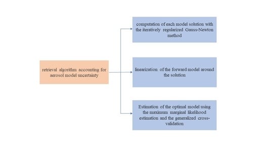
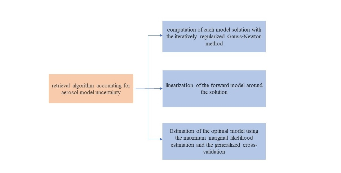
• an iteratively regularized Gauss–Newton method for computing the solution of each model and estimating the ratio of the data error variance and the a priori state variance;
• a linearization of the forward model around the solution for integrating the likelihood density over the state vector;
• parameter choice methods from linear regularization theory for estimating the optimal model and the data error variance.

The paper is organized as follows. In Section 2, we derive a scaled data model with white noise in order to simplify the subsequent analysis. Section 3 is devoted to a review of the Bayesian parameter estimation and model selection in order to describe the problem and clarify the nomenclature. In Section 4, we summarize the iteratively regularized Gauss–Newton method and emphasize some special features of this method, including the estimation of the ratio of the data error variance and the a priori state variance. In Section 5, we assume a linearization of the forward model around the solution and, under this assumption, extend some regularization parameter choice methods for linear problems (the maximum marginal likelihood estimation and the generalized cross-validation) for data error variance estimation and model selection. Section 6 summarizes the computational steps of the proposed retrieval algorithm. In Section 7, we apply the algorithm to the retrieval of aerosol optical thickness and aerosol layer height from the Earth Polychromatic Imaging Camera (EPIC)/Deep Space Climate Observatory (DSCOVR) measurements.

2. Data Model

Consider $N_{\mathrm{m}}$ microphysical models, and let ${\mathbf{F}}_m\left(\mathbf{x}\right)\in {\mathbb{R}}^M$ be the forward model corresponding to the model m for $m=1,\dots ,N_{\mathrm{m}}$. More specifically, in our analysis, ${\mathbf{F}}_m\left(\mathbf{x}\right)$ is the vector of the logarithms of the simulated radiances at all wavelengths ${\lambda }_i$, $i=1,\dots ,M$, i.e., ${\left[{\mathbf{F}}_m\left(\mathbf{x}\right)\right]}_i=ln{I}_m({\lambda }_i,\mathbf{x})$, and $\mathbf{x}\in {\mathbb{R}}^N$ is the state vector encapsulating the atmospheric parameters to be retrieved, e.g., aerosol optical thickness and layer height.

The nonlinear data model under examination consists of the equations:

$${\mathbf{y}}^{\delta }=\mathbf{y}+{\delta }_{\mathrm{mes}},$$

(1)

and:

$$\mathbf{y}={\mathbf{F}}_m\left(\mathbf{x}\right)+{\delta }_{\mathrm{aer}m}$$

(2)

where ${\mathbf{y}}^{\delta }\in {\mathbb{R}}^M$ is the measurement vector or the noisy data vector, $\mathbf{y}$ the exact data vector, ${\delta }_{\mathrm{mes}}\in {\mathbb{R}}^M$ the measurement error vector, and ${\delta }_{\mathrm{aer}m}\in {\mathbb{R}}^M$ the model error vector, i.e., the error due to an inadequate model. Defining the (total) data error vector by:

$${\delta }_m={\delta }_{\mathrm{mes}}+{\delta }_{\mathrm{aer}m},$$

the data model (1) and (2) becomes:

$${\mathbf{y}}^{\delta }={\mathbf{F}}_m\left(\mathbf{x}\right)+{\delta }_m.$$

(3)

In a deterministic setting, ${\delta }_m$ is characterized by the noise level ${\Delta }_m$ (defined as an upper bound for ${\delta }_m$, i.e., $\Vert {\delta }_m\Vert \le {\Delta }_m$), $\mathbf{x}$ is a deterministic vector, and we are faced with the solution of the nonlinear equation ${\mathbf{y}}^{\delta }={\mathbf{F}}_m\left(\mathbf{x}\right)$. In a stochastic setting, ${\delta }_m$ and $\mathbf{x}$ are random vectors, and the data model (3) is solved by means of a Bayesian approach.

Using the prewhitening technique, we transform the data model (3) into a model with white noise. For this purpose, we take:

• ${\delta }_{\mathrm{mes}}$ as a Gaussian random vector with zero mean and covariance matrix:

  $$\begin{array}{cc}\hfill {\mathbf{C}}_{\mathrm{mes}}& =\mathrm{diag}{\left({\sigma }_{\mathrm{mes}i}^2\right)}_M={\sigma }_{\mathrm{mes}}^2{\mathcal{C}}_{\mathrm{mes}},\hfill \\ \hfill {\mathcal{C}}_{\mathrm{mes}}& =\mathrm{diag}{\left(\frac{{\sigma }_{\mathrm{mes}i}^2}{{\sigma }_{\mathrm{mes}}^2}\right)}_M,{\sigma }_{\mathrm{mes}}^2=\frac{1}{M}\sum _{i=1}^M{\sigma }_{\mathrm{mes}i}^2,\hfill \end{array}$$

  and
• ${\delta }_{\mathrm{aer}m}$ as a Gaussian random vector with zero mean and covariance matrix:

  $${\mathbf{C}}_{\mathrm{aer}m}={\sigma }_{\mathrm{aer}m}^2{\mathbf{I}}_M.$$

If ${\delta }_{\mathrm{mes}}$ and ${\delta }_{\mathrm{aer}m}$ are independent random vectors, then ${\delta }_m$ is a Gaussian random vector with zero mean and covariance matrix:

$$\begin{array}{cc}\hfill {\mathbf{C}}_{\delta m}& ={\mathbf{C}}_{\mathrm{mes}}+{\mathbf{C}}_{\mathrm{aer}m}={\sigma }_m^2{\mathcal{C}}_{\delta m},\hfill \\ \hfill {\mathcal{C}}_{\delta m}& =w_{\mathrm{mes}m}{\mathcal{C}}_{\mathrm{mes}}+(1-w_{\mathrm{mes}m}){\mathbf{I}}_M,\hfill \end{array}$$

where:

$$\begin{array}{cc}\hfill {\sigma }_m^2& ={\sigma }_{\mathrm{mes}}^2+{\sigma }_{\mathrm{aer}m}^2\hfill \end{array}$$

is the variance of the data error vector and:

$$\begin{array}{cc}\hfill w_{\mathrm{mes}m}& ={\sigma }_{\mathrm{mes}}^2/{\sigma }_m^2\hfill \end{array}$$

is the weighting factor giving the contribution of ${\mathcal{C}}_{\mathrm{mes}}$ to the covariance matrix ${\mathcal{C}}_{\delta m}$. After these preliminary constructions, we introduce the scaled data model:

$${\overline{\mathbf{y}}}^{\delta }={\overline{\mathbf{F}}}_m\left(\mathbf{x}\right)+{\overline{\delta }}_m,$$

(4)

where:

$${\overline{\mathbf{y}}}^{\delta }=\mathbf{P}{\mathbf{y}}^{\delta },{\overline{\mathbf{F}}}_m\left(\mathbf{x}\right)=\mathbf{P}{\mathbf{F}}_m\left(\mathbf{x}\right),{\overline{\delta }}_m=\mathbf{P}{\delta }_m,$$

and:

$$\mathbf{P}={\mathcal{C}}_{\delta m}^{-1/2}=\mathrm{diag}{\left({\left[1-w_{\mathrm{mes}m}\left(1-\frac{{\sigma }_{\mathrm{mes}i}^2}{{\sigma }_{\mathrm{mes}}^2}\right)\right]}^{-1/2}\right)}_M$$

(5)

is the scaling matrix. Taking into account that:

$${\overline{\mathbf{C}}}_{\delta m}=\mathcal{E}\left\{{\overline{\delta }}_m{\overline{\delta }}_{mk}^T\right\}={\sigma }_m^2\mathbf{P}{\mathcal{C}}_{\delta m}{\mathbf{P}}^{\mathrm{T}}={\sigma }_m^2{\mathbf{I}}_M,$$

we see that by means of the prewhitening technique, the Gaussian random vector ${\delta }_m\sim \mathsf{N}(\mathbf{0},{\mathbf{C}}_{\delta m}={\sigma }_m^2{\mathcal{C}}_{\delta m})$ is transformed into the white noise ${\overline{\delta }}_m\sim \mathsf{N}(\mathbf{0},{\overline{\mathbf{C}}}_{\delta m}={\sigma }_m^2{\mathbf{I}}_M)$. Here and in the following, the notation $\mathsf{N}({\mathbf{x}}_{\mathrm{mean}},{\mathbf{C}}_{\mathrm{x}})$ stands for a normal distribution with mean ${\mathbf{x}}_{\mathrm{mean}}$ and covariance matrix ${\mathbf{C}}_{\mathrm{x}}$.

The following comments can be taken into consideration:

• In [3], the covariance matrix ${\mathbf{C}}_{\mathrm{aer}m}$ was estimated by empirically exploring a set of residuals of model fits to the measurements. Essentially, ${\mathbf{C}}_{\mathrm{aer}m}$ is assumed to be in the form:

  $${\left[{\mathbf{C}}_{\mathrm{aer}m}\right]}_{ij}=\left\{\begin{array}{c}{\sigma }_1^{2}exp[-{({\lambda }_i-{\lambda }_j)}^2/l^2],i\ne j\hfill \\ \\ {\sigma }_0^2+{\sigma }_1^2,i=j\hfill \end{array}\right.,$$

  (6)

  where ${\sigma }_0^2$, ${\sigma }_1^2$, and l (representing the non-spectral diagonal variance, the spectral variance, and the correlation length, respectively) are computed by means of an empirical semivariogram, i.e., the variances of the residual differences are calculated for each wavelength pair with the distance $d=|{\lambda }_i-{\lambda }_j|$, and a theoretical Gaussian variogram model is fitted to these empirical semivariogram values. As compared to Equation (6), in our analysis, we use the diagonal matrix approximation ${\mathbf{C}}_{\mathrm{aer}m}\approx {\sigma }_{\mathrm{aer}m}^2{\mathbf{I}}_M$ with ${\sigma }_{\mathrm{aer}m}^2={\sigma }_0^2+{\sigma }_1^2$.
• In principle, the scaling matrix $\mathbf{P}$ depends on the model error variance ${\sigma }_{\mathrm{aer}m}^2$ through the weighting factor $w_{\mathrm{mes}m}$. However, for ${\left[{\mathbf{F}}_m\left(\mathbf{x}\right)\right]}_i=ln{I}_m({\lambda }_i,\mathbf{x})$, we usually have ${\sigma }_{\mathrm{mes}i}^2\approx {\sigma }_{\mathrm{mes}}^2$ for all $i=1,\dots ,M$. In this case, it follows that ${\mathcal{C}}_{\mathrm{mes}}$, together with ${\mathcal{C}}_{\delta m}$ and $\mathbf{P}$, are close to the identity matrix. This result does not mean that in our model, ${\sigma }_{\mathrm{aer}m}^2$ does not play any role; ${\sigma }_{\mathrm{aer}m}^2$ is included in ${\sigma }_m^2$, which is the subject of an estimation process.

3. Bayesian Approach

In this section, we review the basics of Bayesian parameter estimation and model selection by following the analysis given in Refs. [2,3].

3.1. Bayesian Parameter Estimation

In statistical inversion theory, the state vector $\mathbf{x}$ is assumed to be a random vector, and in this regard, we take $\mathbf{x}\sim \mathsf{N}({\mathbf{x}}_{\mathrm{a}},{\mathbf{C}}_{\mathrm{x}})$, where ${\mathbf{x}}_{\mathrm{a}}$ is the a priori state vector, the best beforehand estimate of the solution, and:

$$\begin{array}{cc}\hfill {\mathbf{C}}_{\mathrm{x}}& =\mathrm{diag}{\left({\sigma }_{\mathrm{x}i}^2\right)}_N={\sigma }_{\mathrm{x}}^2{\mathcal{C}}_{\mathrm{x}},\hfill \\ \hfill {\mathcal{C}}_{\mathrm{x}}& =\mathrm{diag}{\left(\frac{{\sigma }_{\mathrm{x}i}^2}{{\sigma }_{\mathrm{x}}^2}\right)}_N,{\sigma }_{\mathrm{x}}^2=\frac{1}{N}\sum _{i=1}^N{\sigma }_{\mathrm{x}i}^2.\hfill \end{array}$$

Furthermore, the matrix $\mathbf{L}$ is defined through the Cholesky factorization:

$${\mathcal{C}}_{\mathrm{x}}^{-1}={\mathbf{L}}^{\mathrm{T}}\mathbf{L},\mathrm{that}\mathrm{is},\mathbf{L}=\mathrm{diag}{\left(\frac{{\sigma }_{\mathrm{x}}}{{\sigma }_{\mathrm{x}i}}\right)}_N,$$

and the parameter $\alpha$ is defined as:

$$\alpha =\frac{{\sigma }_m^2}{{\sigma }_{\mathrm{x}}^2}.$$

(7)

The data model (3) gives a relation between the three random vectors ${\overline{\mathbf{y}}}^{\delta }$, $\mathbf{x}$, and ${\delta }_m$, and therefore, their probability densities depend on each other. The following probability densities are relevant in Bayesian parameter estimation: (i) the a priori density $p(\mathbf{x}\mid m)$, which represents the conditional probability density of $\mathbf{x}$ given the model m before performing the measurement ${\overline{\mathbf{y}}}^{\delta }$, (ii) the likelihood density $p({\overline{\mathbf{y}}}^{\delta }\mid \mathbf{x},m)$, which represents the conditional probability density of ${\overline{\mathbf{y}}}^{\delta }$ given the state $\mathbf{x}$ and the model m, and (iii) the a posteriori density $p(\mathbf{x}\mid {\overline{\mathbf{y}}}^{\delta },m)$, which represents the conditional probability density of $\mathbf{x}$ given the data ${\overline{\mathbf{y}}}^{\delta }$ and the model m.

The Bayes theorem of inverse problems relates the a posteriori density to the likelihood density:

$$\begin{array}{cc}\hfill p(\mathbf{x}\mid {\overline{\mathbf{y}}}^{\delta },m)& =\frac{p({\overline{\mathbf{y}}}^{\delta }\mid \mathbf{x},m)p(\mathbf{x},m)}{p({\overline{\mathbf{y}}}^{\delta },m)}\hfill \\ \hfill & =\frac{p({\overline{\mathbf{y}}}^{\delta }\mid \mathbf{x},m)p(\mathbf{x}\mid m)}{p({\overline{\mathbf{y}}}^{\delta }\mid m)}.\hfill \end{array}$$

In Bayesian parameter estimation, the marginal likelihood density $p({\overline{\mathbf{y}}}^{\delta }\mid m)$, defined by:

$$p({\overline{\mathbf{y}}}^{\delta }\mid m)=\int p(\mathbf{x},{\overline{\mathbf{y}}}^{\delta }\mid m)\mathrm{d}\mathbf{x}=\int p({\overline{\mathbf{y}}}^{\delta }\mid \mathbf{x},m)p(\mathbf{x}\mid m)\mathrm{d}\mathbf{x},$$

(8)

plays the role of a normalization constant and is usually ignored. However, as we will see in the next section, this density is of particular importance in Bayesian model selection.

For $\mathbf{x}\sim \mathsf{N}({\mathbf{x}}_{\mathrm{a}},{\mathbf{C}}_{\mathrm{x}}={\sigma }_m^2{\left(\alpha {\mathbf{L}}^{\mathrm{T}}\mathbf{L}\right)}^{-1})$ and ${\overline{\delta }}_m\sim \mathsf{N}(\mathbf{0},{\overline{\mathbf{C}}}_{\delta m}={\sigma }_m^2{\mathbf{I}}_M)$, the probability densities $p(\mathbf{x}\mid m)$ and $p({\overline{\mathbf{y}}}^{\delta }\mid \mathbf{x},m)$ are given by:

$$\begin{array}{cc}\hfill p(\mathbf{x}\mid m)& =\frac{1}{\sqrt{{\left(2\pi {\sigma }_m^2\right)}^{N}det\left[{\left(\alpha {\mathbf{L}}^{\mathrm{T}}\mathbf{L}\right)}^{-1}\right]}}\hfill \\ \hfill & \times exp\left[-\frac{\alpha }{2{\sigma }_m^2}\Vert \mathbf{L}(\mathbf{x}-{\mathbf{x}}_{\mathrm{a}}){\Vert }^2\right]\hfill \end{array}$$

(9)

and:

$$\begin{array}{cc}\hfill p({\overline{\mathbf{y}}}^{\delta }\mid \mathbf{x},m)& =\frac{1}{\sqrt{{\left(2\pi {\sigma }_m^2\right)}^M}}exp\left[-\frac{1}{2{\sigma }_m^2}\Vert {\overline{\mathbf{y}}}^{\delta }-{\overline{\mathbf{F}}}_m\left(\mathbf{x}\right){\Vert }^2\right],\hfill \end{array}$$

(10)

respectively. The Bayes formula yields the following expression for the a posteriori density:

$$p(\mathbf{x}\mid {\overline{\mathbf{y}}}^{\delta },m)\propto exp\left[-\frac{1}{2}{V}_{\alpha }(\mathbf{x}\mid {\overline{\mathbf{y}}}^{\delta },m)\right],$$

(11)

where the a posteriori potential $V_{\alpha }(\mathbf{x}\mid {\overline{\mathbf{y}}}^{\delta },m)$ is defined by:

$$V_{\alpha }(\mathbf{x}\mid {\overline{\mathbf{y}}}^{\delta },m)=\frac{1}{{\sigma }_m^2}\left[{∥{\overline{\mathbf{y}}}^{\delta }-{\overline{\mathbf{F}}}_m\left(\mathbf{x}\right)∥}^2+\alpha {∥\mathbf{L}(\mathbf{x}-{\mathbf{x}}_{\mathrm{a}})∥}^2\right].$$

(12)

The maximum a posteriori estimator ${\widehat{\mathbf{x}}}_{m\alpha }^{\delta }$ maximizing the conditional probability density $p(\mathbf{x}\mid {\overline{\mathbf{y}}}^{\delta },m)$ also minimizes the potential $V_{\alpha }(\mathbf{x}\mid {\overline{\mathbf{y}}}^{\delta },m)$, i.e.,

$${\widehat{\mathbf{x}}}_{m\alpha }^{\delta }=arg\underset{\mathbf{x}}{min}{V}_{\alpha }(\mathbf{x}\mid {\overline{\mathbf{y}}}^{\delta },m).$$

(13)

3.2. Bayesian Model Selection

The relative evidence, also known as the a posteriori probability of the model m given the measurement ${\mathbf{y}}^{\delta }$, $p(m\mid {\overline{\mathbf{y}}}^{\delta })$, is used for model comparison. By taking into consideration the Bayes theorem, this conditional probability density is defined by:

$$p(m\mid {\overline{\mathbf{y}}}^{\delta })=\frac{p({\overline{\mathbf{y}}}^{\delta }\mid m)p\left(m\right)}{p\left({\overline{\mathbf{y}}}^{\delta }\right)}.$$

The mean formula:

$$p\left({\overline{\mathbf{y}}}^{\delta }\right)=\sum _{m=1}^{N_{\mathrm{m}}}p({\overline{\mathbf{y}}}^{\delta }\mid m)p\left(m\right)$$

and the assumption that all models are equally likely, i.e., $p\left(m\right)=1/N_{\mathrm{m}}$, yield:

$$\begin{array}{cc}\hfill p(m\mid {\overline{\mathbf{y}}}^{\delta })& =\frac{p({\overline{\mathbf{y}}}^{\delta }\mid m)}{{\sum }_{m=1}^{N_{\mathrm{m}}}p({\overline{\mathbf{y}}}^{\delta }\mid m)}.\hfill \end{array}$$

(14)

Intuitively, the model with the highest evidence is the best among all the models involved, and in this regard, we define the maximum solution estimate as:

$${\widehat{\mathbf{x}}}_{\max }^{\delta }={\widehat{\mathbf{x}}}_{m^{☆}\alpha }^{\delta },m^{☆}=arg\underset{m}{max}p(m\mid {\overline{\mathbf{y}}}^{\delta }).$$

(15)

In fact, we can compare the models to see if one of them clearly shows the highest evidence, or if there are several models with comparable values of evidence. When several models can provide equally good fits to the measurement, we can use the Bayesian model averaging technique to combine the individual a posteriori densities weighted by their evidence. Specifically, using the relation:

$$\begin{array}{cc}\hfill p(\mathbf{x},{\overline{\mathbf{y}}}^{\delta })& =\sum _{m=1}^{N_{\mathrm{m}}}p(\mathbf{x},{\overline{\mathbf{y}}}^{\delta },m)\hfill \\ \hfill & =\sum _{m=1}^{N_{\mathrm{m}}}p(\mathbf{x}\mid {\overline{\mathbf{y}}}^{\delta },m)p(m\mid {\overline{\mathbf{y}}}^{\delta })p\left({\overline{\mathbf{y}}}^{\delta }\right)\hfill \end{array}$$

on the one hand, and $p(\mathbf{x},{\overline{\mathbf{y}}}^{\delta })=p(\mathbf{x}\mid {\overline{\mathbf{y}}}^{\delta })p\left({\overline{\mathbf{y}}}^{\delta }\right)$, on the other hand, we are led to the Bayesian model averaging formula:

$$p_{\mathrm{mean}}(\mathbf{x}\mid {\overline{\mathbf{y}}}^{\delta })=\sum _{m=1}^{N_{\mathrm{m}}}p(\mathbf{x}\mid {\overline{\mathbf{y}}}^{\delta },m)p(m\mid {\overline{\mathbf{y}}}^{\delta }),$$

(16)

and, consequently, to the mean solution estimate:

$${\widehat{\mathbf{x}}}_{\mathrm{mean}}^{\delta }=\sum _{m=1}^{N_{\mathrm{m}}}{\widehat{\mathbf{x}}}_{m\alpha }^{\delta }p(m\mid {\overline{\mathbf{y}}}^{\delta }).$$

(17)

The above analysis shows that in Bayesian parameter estimation and model selection, we are faced with the following problems:

Problem 1.

From Equations (11)–(13), it is apparent that the computation of the estimator ${\widehat{\mathbf{x}}}_{m\alpha }^{\delta }$ requires the knowledge of the parameter $\alpha$, i.e., the ratio of the data error variance and the a priori state variance.

Problem 2.

From Equations (15) and (17), we see that the solution estimates ${\widehat{\mathbf{x}}}_{\max }^{\delta }$ and ${\widehat{\mathbf{x}}}_{\mathrm{mean}}^{\delta }$ are expressed in terms of relative evidence $p(m\mid {\overline{\mathbf{y}}}^{\delta })$, which in turn, according to Equation (14), is expressed in terms of the marginal likelihood density $p({\overline{\mathbf{y}}}^{\delta }\mid m)$. In view of Equation (8), the computation of the marginal likelihood density $p({\overline{\mathbf{y}}}^{\delta }\mid m)$ requires the knowledge of the likelihood density $p({\overline{\mathbf{y}}}^{\delta }\mid \mathbf{x},m)$, and therefore of Equation (10), of the data error variance ${\sigma }_m^2$.

Problem 3.

The dependency of the likelihood density $p({\overline{\mathbf{y}}}^{\delta }\mid \mathbf{x},m)$ on the nonlinear forward model ${\overline{\mathbf{F}}}_m\left(\mathbf{x}\right)$ does not allow an analytical integration in Equation (8).

4. Iteratively Regularized Gauss–Newton Method

In the framework of Tikhonov regularization, a regularized solution ${\mathbf{x}}_{m\alpha }^{\delta }$ to the nonlinear equation ${\overline{\mathbf{y}}}^{\delta }={\overline{\mathbf{F}}}_m\left(\mathbf{x}\right)$ is computed as the minimizer of the Tikhonov function:

$${\mathcal{F}}_{m\alpha }\left(\mathbf{x}\right)={∥{\overline{\mathbf{y}}}^{\delta }-{\overline{\mathbf{F}}}_m\left(\mathbf{x}\right)∥}^2+\alpha {∥\mathbf{L}(\mathbf{x}-{\mathbf{x}}_{\mathrm{a}})∥}^2,$$

(18)

that is,

$${\mathbf{x}}_{m\alpha }^{\delta }=arg\underset{\mathbf{x}}{min}{\mathcal{F}}_{m\alpha }\left(\mathbf{x}\right).$$

(19)

In classical regularization theory, the first term on the right-hand side of Equation (18) is the squared residual; the second one is the penalty term; while $\alpha$ and $\mathbf{L}$ are the regularization parameter and the regularization matrix, respectively. From Equations (12) and (18), we see that $V_{\alpha }(\mathbf{x}\mid {\overline{\mathbf{y}}}^{\delta },m)=(1/{\sigma }_m^2){\mathcal{F}}_{m\alpha }\left(\mathbf{x}\right)$, and from Equations (13) and (19), we deduce that ${\widehat{\mathbf{x}}}_{m\alpha }^{\delta }={\mathbf{x}}_{m\alpha }^{\delta }$. Thus, the maximum a posteriori estimate coincides with the Tikhonov solution, and therefore, the Bayesian parameter estimation can be regarded as a stochastic version of the method of Tikhonov regularization with an a priori chosen regularization parameter $\alpha$.

In the framework of Tikhonov regularization, the computation of the optimal regularization parameter is a crucial issue. With too little regularization, reconstructions deviate significantly from the a priori, and the solution is said to be under-regularized. With too much regularization, the reconstructions are too close to the a priori, and the solution is said to be over-regularized. In the Bayesian framework, the optimal regularization parameter is identified as the true ratio of the data error variance and the a priori state variance.

Several regularization parameter choice methods were discussed in [5]. These include methods with constant regularization parameters, e.g., the maximum likelihood estimation, the generalized cross-validation, and the nonlinear L-curve method. Unfortunately, at present, there is no fail-safe regularization parameter choice method that guarantees small solution errors in any circumstance, that is for any errors in the data vector.

An improvement of the problems associated with the regularization parameter selection is achieved in the framework of the so-called iterative regularization methods. These approaches are less sensitive to overestimates of the regularization parameter, but require more iteration steps to achieve convergence. A representative iterative approach is the iteratively regularized Gauss–Newton method.

At iteration step k of the iteratively regularized Gauss–Newton method, the forward model ${\overline{\mathbf{F}}}_m\left(\mathbf{x}\right)$ is linearized around the current iterate ${\mathbf{x}}_{mk}^{\delta }$,

$${\overline{\mathbf{F}}}_m\left(\mathbf{x}\right)\approx {\overline{\mathbf{F}}}_m\left({\mathbf{x}}_{mk}^{\delta }\right)+{\overline{\mathbf{K}}}_{mk}(\mathbf{x}-{\mathbf{x}}_{mk}^{\delta }),$$

where:

$${\overline{\mathbf{K}}}_{mk}=\frac{\partial {\overline{\mathbf{F}}}_m}{\partial \mathbf{x}}\left({\mathbf{x}}_{mk}^{\delta }\right)$$

is the Jacobian matrix at ${\mathbf{x}}_{mk}^{\delta }$, and the nonlinear equation ${\overline{\mathbf{F}}}_m\left(\mathbf{x}\right)={\overline{\mathbf{y}}}^{\delta }$ is replaced by its linearization:

$${\overline{\mathbf{K}}}_{mk}\mathbf{p}={\overline{\mathbf{y}}}_{mk}^{\delta },$$

(20)

where:

$$\mathbf{p}=\mathbf{x}-{\mathbf{x}}_{\mathrm{a}}$$

is the step vector with respect to the a priori and:

$${\overline{\mathbf{y}}}_{mk}^{\delta }={\overline{\mathbf{y}}}^{\delta }-{\overline{\mathbf{F}}}_m\left({\mathbf{x}}_{mk}^{\delta }\right)+{\overline{\mathbf{K}}}_{mk}({\mathbf{x}}_{mk}^{\delta }-{\mathbf{x}}_{\mathrm{a}})$$

is the linearized data vector at iteration step k.

Since the nonlinear problem is ill-posed, its linearization is also ill-posed. Therefore, the linearized Equation (20) is solved by means of Tikhonov regularization with the penalty term ${\alpha }_k{\Vert \mathbf{L}\mathbf{p}\Vert }^2$, where the regularization parameters ${\alpha }_k$ are the terms of a decreasing (geometric) sequence, i.e., ${\alpha }_k=q{\alpha }_{k-1}$ with $q<1$. Note that in the method of Tikhonov regularization, the regularization parameter $\alpha$ is kept constant during the iterative process. The Tikhonov function for the linearized equation takes the form:

$${\mathcal{F}}_{\mathrm{l}mk}\left(\mathbf{p}\right)={∥{\overline{\mathbf{y}}}_{mk}^{\delta }-{\overline{\mathbf{K}}}_{mk}\mathbf{p}∥}^2+{\alpha }_k{∥\mathbf{L}\mathbf{p}∥}^2,$$

and its minimizer is given by:

$${\mathbf{p}}_{mk}^{\delta }={\overline{\mathbf{K}}}_{mk}^{†}{\overline{\mathbf{y}}}_{mk}^{\delta },$$

where:

$${\overline{\mathbf{K}}}_{mk}^{†}={({\overline{\mathbf{K}}}_{mk}^{\mathrm{T}}{\overline{\mathbf{K}}}_{mk}+{\alpha }_k{\mathbf{L}}^{\mathrm{T}}\mathbf{L})}^{-1}{\overline{\mathbf{K}}}_{mk}^{\mathrm{T}}$$

is the regularized generalized inverse at ${\mathbf{x}}_{mk}^{\delta }$. The new iterate is computed as:

$${\mathbf{x}}_{mk+1}^{\delta }={\mathbf{x}}_{\mathrm{a}}+{\overline{\mathbf{K}}}_{mk}^{†}{\overline{\mathbf{y}}}_{mk}^{\delta }.$$

For the iterative regularization methods, the number of iteration steps k plays the role of the regularization parameter, and the iterative process is stopped after an appropriate number of steps $k^{☆}$ in order to avoid an uncontrolled expansion of errors in the data. In fact, a mere minimization of the residual $\Vert {\mathbf{r}}_{mk}^{\delta }\Vert$, where:

$${\mathbf{r}}_{mk}^{\delta }={\overline{\mathbf{y}}}^{\delta }-{\overline{\mathbf{F}}}_m\left({\mathbf{x}}_{mk}^{\delta }\right)$$

is the residual vector at ${\mathbf{x}}_{mk}^{\delta }$, leads to a semi-convergent behavior of the iterated solution: while the error in the residual decreases as the number of iteration steps increases, the error in the solution starts to increase after an initial decay. A widely used a posteriori choice for the stopping index $k^{☆}$ is the discrepancy principle. According to this principle, the iterative process is terminated after $k^{☆}$ steps such that:

$${∥{\mathbf{r}}_{m{k}^{☆}}^{\delta }∥}^2\le \eta {\Delta }_m^2<{∥{\mathbf{r}}_{mk}^{\delta }∥}^2,0\le k<k^{☆},$$

with $\eta >1$; hence, the regularized solution is ${\mathbf{x}}_{m{k}^{☆}}^{\delta }$. Since the noise level cannot be estimated a priori for many practical problems arising in atmospheric remote sensing, we adopt a practical approach. This is based on the observation that the squared residual $\Vert {\mathbf{r}}_{mk}^{\delta }{\Vert }^2$ decreases during the iterative process and attains a plateau at approximately ${\Delta }_m^2$. Thus, if the nonlinear residuals $\Vert {\mathbf{r}}_{mk}^{\delta }\Vert$ converge to $\Vert {\mathbf{r}}_{m\infty }^{\delta }\Vert$ within a prescribed tolerance, we use the estimate:

$${\Delta }_m^2=\Vert {\mathbf{r}}_{m\infty }^{\delta }{\Vert }^2.$$

The above heuristic stopping rule does not have any mathematical justification, but works sufficiently well in practice.

Since the amount of regularization is gradually decreased during the iterative processes, the iteratively regularized Gauss–Newton method can handle problems that practically do not require much regularization.

The numerical experiments performed in [5] showed that at the solution ${\mathbf{x}}_{m{k}^{☆}}^{\delta }$, (i) ${\alpha }_{k^{☆}-1}$ is close to the optimal regularization parameter, and (ii) ${\mathbf{x}}_{m{k}^{☆}}^{\delta }$ is close to the Tikhonov solution corresponding to the optimal regularization parameter. In this regard, we make the following assumptions:

• $\widehat{\alpha }={\alpha }_{k^{☆}-1}$ is an estimate for the optimal regularization parameter, and
• ${\mathbf{x}}_{m\widehat{\alpha }}^{\delta }={\mathbf{x}}_{m{k}^{☆}}^{\delta }$ is the minimizer of the Tikhonov function with regularization parameter $\widehat{\alpha }$, ${\mathcal{F}}_{m\widehat{\alpha }}\left(\mathbf{x}\right)$.

Some consequences of the second assumption are the following. The optimality condition $\nabla {\mathcal{F}}_{m\widehat{\alpha }}\left({\mathbf{x}}_{m\widehat{\alpha }}^{\delta }\right)=0$, yields:

$${\overline{\mathbf{K}}}_{m\widehat{\alpha }}^{\mathrm{T}}[{\overline{\mathbf{F}}}_m\left({\mathbf{x}}_{m\widehat{\alpha }}^{\delta }\right)-{\overline{\mathbf{y}}}^{\delta }]+\widehat{\alpha }\mathbf{L}{\mathbf{L}}^T({\mathbf{x}}_{m\widehat{\alpha }}^{\delta }-{\mathbf{x}}_{\mathrm{a}})=0$$

and further,

$${\mathbf{x}}_{m\widehat{\alpha }}^{\delta }={\mathbf{x}}_{\mathrm{a}}+{\overline{\mathbf{K}}}_{m\widehat{\alpha }}^{†}{\overline{\mathbf{y}}}_{m\widehat{\alpha }}^{\delta },$$

where ${\overline{\mathbf{K}}}_{m\widehat{\alpha }}={\overline{\mathbf{K}}}_{m{k}^{☆}}$,

$${\overline{\mathbf{y}}}_{m\widehat{\alpha }}^{\delta }={\overline{\mathbf{y}}}_{m{k}^{☆}}^{\delta }={\overline{\mathbf{y}}}^{\delta }-{\overline{\mathbf{F}}}_m\left({\mathbf{x}}_{m\widehat{\alpha }}^{\delta }\right)+{\overline{\mathbf{K}}}_{m\widehat{\alpha }}({\mathbf{x}}_{m\widehat{\alpha }}^{\delta }-{\mathbf{x}}_{\mathrm{a}}),$$

(21)

and:

$${\overline{\mathbf{K}}}_{m\widehat{\alpha }}^{†}={({\overline{\mathbf{K}}}_{m\widehat{\alpha }}^{\mathrm{T}}{\overline{\mathbf{K}}}_{m\widehat{\alpha }}+\widehat{\alpha }{\mathbf{L}}^{\mathrm{T}}\mathbf{L})}^{-1}{\overline{\mathbf{K}}}_{m\widehat{\alpha }}^{\mathrm{T}}.$$

(22)

Consequently, we see that:

$${\mathbf{p}}_{m\widehat{\alpha }}^{\delta }={\mathbf{x}}_{m\widehat{\alpha }}^{\delta }-{\mathbf{x}}_{\mathrm{a}}={\overline{\mathbf{K}}}_{m\widehat{\alpha }}^{†}{\overline{\mathbf{y}}}_{m\widehat{\alpha }}^{\delta }$$

(23)

is the minimizer of the Tikhonov function:

$${\mathcal{F}}_{\mathrm{l}m\widehat{\alpha }}\left(\mathbf{p}\right)={∥{\overline{\mathbf{y}}}_{m\widehat{\alpha }}^{\delta }-{\overline{\mathbf{K}}}_{m\widehat{\alpha }}\mathbf{p}∥}^2+\widehat{\alpha }{∥\mathbf{L}\mathbf{p}∥}^2,$$

and that the residual vector of the linear equation ${\overline{\mathbf{y}}}_{m\widehat{\alpha }}^{\delta }={\overline{\mathbf{K}}}_{m\widehat{\alpha }}\mathbf{p}$ is equal to the nonlinear residual vector at the solution, i.e.,

$${\overline{\mathbf{y}}}_{m\widehat{\alpha }}^{\delta }-{\overline{\mathbf{K}}}_{m\widehat{\alpha }}{\mathbf{p}}_{m\widehat{\alpha }}^{\delta }={\overline{\mathbf{y}}}^{\delta }-{\overline{\mathbf{F}}}_m\left({\mathbf{x}}_{m\widehat{\alpha }}^{\delta }\right)={\mathbf{r}}_{m\widehat{\alpha }}^{\delta }.$$

(24)

In summary, in the iteratively regularized Gauss–Newton method:

• the computation of the regularized solution ${\mathbf{x}}_{m\widehat{\alpha }}^{\delta }$ depends only on the initial value ${\alpha }_1$ and the ratio q of the geometric sequence ${\alpha }_k,$ which determine the rate of convergence, and
• the regularization parameter at the solution is an estimate for the optimal regularization parameter, and so, for the ratio of the data error variance and the a priori state variance.

Taking these results into account, we may conclude that the iteratively regularized Gauss–Newton method gives a solution to Problem 1 of the Bayesian parameter estimation.

5. Parameter Estimation and Model Selection

In this section, we address Problems 2 and 3 related to Bayesian model selection.

To solve Problem 3, we suppose that the forward model can be linearized around the solution ${\mathbf{x}}_{m\widehat{\alpha }}^{\delta }$ [6]. In other words, in the first-order Taylor expansion:

$${\overline{\mathbf{F}}}_m\left(\mathbf{x}\right)={\overline{\mathbf{F}}}_m\left({\mathbf{x}}_{m\widehat{\alpha }}^{\delta }\right)+{\overline{\mathbf{K}}}_{m\widehat{\alpha }}(\mathbf{x}-{\mathbf{x}}_{m\widehat{\alpha }}^{\delta })+{\overline{\mathbf{R}}}_m(\mathbf{x},{\mathbf{x}}_{m\widehat{\alpha }}^{\delta })$$

(25)

the remainder term ${\overline{\mathbf{R}}}_m(\mathbf{x},{\mathbf{x}}_{m\widehat{\alpha }}^{\delta })$ can be neglected. As a result, the nonlinear data model ${\overline{\mathbf{y}}}^{\delta }={\overline{\mathbf{F}}}_m\left(\mathbf{x}\right)+{\overline{\delta }}_m$ becomes the linear model:

$${\overline{\mathbf{y}}}_{m\widehat{\alpha }}^{\delta }={\overline{\mathbf{K}}}_{m\widehat{\alpha }}\mathbf{p}+{\overline{\delta }}_m,$$

(26)

where ${\overline{\mathbf{y}}}_{m\widehat{\alpha }}^{\delta }$ is given by Equation (21), $\mathbf{p}=\mathbf{x}-{\mathbf{x}}_{\mathrm{a}}\sim \mathsf{N}(\mathbf{0},{\mathbf{C}}_{\mathrm{x}}={\sigma }_m^2{\left(\widehat{\alpha }{\mathbf{L}}^{\mathrm{T}}\mathbf{L}\right)}^{-1})$ and ${\overline{\delta }}_m\sim \mathsf{N}(\mathbf{0},{\overline{\mathbf{C}}}_{\delta m}={\sigma }_m^2{\mathbf{I}}_M)$. The direct consequences of dealing with the linear model (26) are the following results:

• the a posteriori density $p(\mathbf{x}\mid {\overline{\mathbf{y}}}^{\delta },m)$ can be expressed as a Gaussian distribution:

  $$p(\mathbf{x}\mid {\overline{\mathbf{y}}}^{\delta },m)\propto exp\left[-\frac{1}{2}{(\mathbf{x}-{\mathbf{x}}_{m\widehat{\alpha }}^{\delta })}^{\mathrm{T}}{\widehat{\mathbf{C}}}_{\mathrm{x}m}^{-1}(\mathbf{x}-{\mathbf{x}}_{m\widehat{\alpha }}^{\delta })\right],$$

  where:

  $${\widehat{\mathbf{C}}}_{\mathtt{x}m}={\sigma }_m^2{({\overline{\mathbf{K}}}_{m\widehat{\alpha }}^{\mathrm{T}}{\overline{\mathbf{K}}}_{m\widehat{\alpha }}+\widehat{\alpha }{\mathbf{L}}^{\mathrm{T}}\mathbf{L})}^{-1}.$$

  (27)

  is the a posteriori covariance matrix, and
• as shown in Appendix A, the marginal likelihood density $p({\overline{\mathbf{y}}}^{\delta }\mid m)$ can be computed analytically; the result is:

  $$\begin{array}{cc}\hfill p({\overline{\mathbf{y}}}^{\delta }\mid m)& =\sqrt{\frac{\det ({\mathbf{I}}_M-{\widehat{\mathbf{A}}}_{m\widehat{\alpha }})}{{\left(2\pi {\sigma }_m^2\right)}^M}}\hfill \\ \hfill & \times exp\left[-\frac{1}{2{\sigma }_m^2}{\overline{\mathbf{y}}}_{m\widehat{\alpha }}^{\delta \mathrm{T}}({\mathbf{I}}_M-{\widehat{\mathbf{A}}}_{m\widehat{\alpha }}){\overline{\mathbf{y}}}_{m\widehat{\alpha }}^{\delta }\right],\hfill \end{array}$$

  (28)

  where ${\widehat{\mathbf{A}}}_{m\widehat{\alpha }}={\overline{\mathbf{K}}}_{m\widehat{\alpha }}{\overline{\mathbf{K}}}_{m\widehat{\alpha }}^{†}$ is the influence matrix at the solution ${\mathbf{x}}_{m\widehat{\alpha }}^{\delta }$.

The replacement of the nonlinear data model by a linear data model will also enable us to deal with Problem 2. More specifically, for this purpose, we will adapt some regularization parameter choice methods for linear problems, i.e., maximum marginal likelihood estimation [7,8,9] and generalized cross-validation [10,11], to model selection. Furthermore, estimates for the data error variance ${\sigma }_m^2$ delivered by these methods will be used to compute the marginal likelihood density and, therefore, the relative evidence.

In Appendix B, it is shown that:

• in the framework of maximum marginal likelihood estimation, the data error variance can be estimated by:

  $${\widehat{\sigma }}_{\mathrm{L}m}^2=\frac{1}{M}{\overline{\mathbf{y}}}_{m\widehat{\alpha }}^{\delta \mathrm{T}}({\mathbf{I}}_M-{\widehat{\mathbf{A}}}_{m\widehat{\alpha }}){\overline{\mathbf{y}}}_{m\widehat{\alpha }}^{\delta },$$

  (29)

  and the model with the smallest value of the marginal likelihood function, defined by:

  $$\lambda \left(m\right)=\frac{{\overline{\mathbf{y}}}_{m\widehat{\alpha }}^{\delta \mathrm{T}}({\mathbf{I}}_M-{\widehat{\mathbf{A}}}_{m\widehat{\alpha }}){\overline{\mathbf{y}}}_{m\widehat{\alpha }}^{\delta }}{\sqrt[M]{\det ({\mathbf{I}}_M-{\widehat{\mathbf{A}}}_{m\widehat{\alpha }})}},$$

  (30)

  is optimal.
• in the framework of generalized cross-validation, the data error variance can be estimated by:

  $${\widehat{\sigma }}_{\mathrm{G}m}^2=\frac{\Vert {\mathbf{r}}_{m\widehat{\alpha }}^{\delta }{\Vert }^2}{\left[\mathrm{trace}({\mathbf{I}}_M-{\widehat{\mathbf{A}}}_{m\widehat{\alpha }})\right]},$$

  (31)

  and the model with the smallest value of the generalized cross-validation function, defined by:

  $$\upsilon \left(m\right)=\frac{\Vert {\mathbf{r}}_{m\widehat{\alpha }}^{\delta }{\Vert }^2}{{\left[\mathrm{trace}(\mathbf{I}-{\widehat{\mathbf{A}}}_{m\widehat{\alpha }})\right]}^2},$$

  (32)

  is optimal.

Denoting by $p_{\mathrm{L}}({\overline{\mathbf{y}}}^{\delta }\mid m)$ and $p_{\mathrm{G}}({\overline{\mathbf{y}}}^{\delta }\mid m)$ the marginal likelihoods corresponding to ${\widehat{\sigma }}_{\mathrm{L}m}^2$ and ${\widehat{\sigma }}_{\mathrm{G}m}^2$, respectively, we define:

• the relative evidence of an approach based on marginal likelihood and the computation of the data error variance in the framework of the Maximum Marginal Likelihood Estimation (MLMMLE) by:

  $$\begin{array}{cc}\hfill p_{\mathrm{MLMMLE}}(m\mid {\mathbf{y}}^{\delta })& =\frac{p_{\mathrm{L}}({\overline{\mathbf{y}}}^{\delta }\mid m)}{{\sum }_{m=1}^{N_{\mathrm{m}}}{p}_{\mathrm{L}}({\overline{\mathbf{y}}}^{\delta }\mid m)},\hfill \end{array}$$

  (33)
• the relative evidence of an approach based on the marginal likelihood and computation of the data error variance in the framework of the Generalized Cross-Validation (MLGCV) by:

  $$\begin{array}{cc}\hfill p_{\mathrm{MLGCV}}(m\mid {\mathbf{y}}^{\delta })& =\frac{p_{\mathrm{G}}({\overline{\mathbf{y}}}_m^{\delta }\mid m)}{{\sum }_{m=1}^{N_{\mathrm{m}}}{p}_{\mathrm{G}}({\overline{\mathbf{y}}}_m^{\delta }\mid m)}.\hfill \end{array}$$

  (34)

Note that for the data error variance estimate (29), the marginal likelihood density becomes:

$$p_{\mathrm{L}}({\overline{\mathbf{y}}}^{\delta }\mid m)=\frac{c_M}{\sqrt{{\left[\lambda \left(m\right)\right]}^M}},$$

with:

$$c_M=\sqrt{{\left(\frac{M}{2\pi }\right)}^M}exp\left(-\frac{M}{2}\right).$$

On the other hand, the statements (30) and (32) are equivalent to (cf. Equation (15)):

$${\widehat{\mathbf{x}}}_{\max }^{\delta }={\mathbf{x}}_{m^{☆}\widehat{\alpha }}^{\delta },m^{☆}=arg\underset{m}{max}\frac{1}{\lambda \left(m\right)},$$

(35)

and:

$${\widehat{\mathbf{x}}}_{\max }^{\delta }={\mathbf{x}}_{m^{☆}\widehat{\alpha }}^{\delta },m^{☆}=arg\underset{m}{max}\frac{1}{v\left(m\right)},$$

(36)

respectively. Deviating from a stochastic interpretation of the relative evidence and regarding this quantity in a deterministic setting merely as a merit function characterizing the solution ${\mathbf{x}}_{m\widehat{\alpha }}^{\delta }$ , we define:

• the relative evidence of an approach based on Maximum Marginal Likelihood Estimation (MMLE) by:

  $$p_{\mathrm{MMLE}}(m\mid {\mathbf{y}}^{\delta })=\frac{1/\lambda \left(m\right)}{{\sum }_{m=1}^{N_{\mathrm{m}}}1/\lambda \left(m\right)},$$

  (37)
• the relative evidence of an approach based on Generalized Cross-Validation (GCV) by:

  $$p_{\mathrm{GCV}}(m\mid {\mathbf{y}}^{\delta })=\frac{1/\upsilon \left(m\right)}{{\sum }_{m=1}^{N_{\mathrm{m}}}1/\upsilon \left(m\right)}.$$

  (38)

Note that $p_{\mathrm{MMLE}}(m\mid {\mathbf{y}}^{\delta })$ and $p_{\mathrm{GCV}}(m\mid {\mathbf{y}}^{\delta })$ do not depend on the data error variance ${\sigma }_m^2$. Note also that ${\widehat{\sigma }}_{\mathrm{G}m}^2$ is defined in terms of the square residual:

$$\begin{array}{cc}\hfill \Vert {\mathbf{r}}_{m\widehat{\alpha }}^{\delta }{\Vert }^2& =\Vert {\overline{\mathbf{y}}}_{m\widehat{\alpha }}^{\delta }-{\overline{\mathbf{K}}}_{m\widehat{\alpha }}{\mathbf{p}}_{m\widehat{\alpha }}^{\delta }{\Vert }^2=\Vert ({\mathbf{I}}_M-{\widehat{\mathbf{A}}}_{m\widehat{\alpha }}){\overline{\mathbf{y}}}_{m\widehat{\alpha }}^{\delta }{\Vert }^2,\hfill \end{array}$$

while, according to Equation (29), ${\widehat{\sigma }}_{\mathrm{L}m}^2$ is defined in terms of the quantity ${\overline{\mathbf{y}}}_{m\widehat{\alpha }}^{\delta \mathrm{T}}({\mathbf{I}}_M-{\widehat{\mathbf{A}}}_{m\widehat{\alpha }}){\overline{\mathbf{y}}}_{m\widehat{\alpha }}^{\delta }$. The same difference exists between the numerators of the cross-validation function $v\left(m\right)$ and the marginal likelihood function $\lambda \left(m\right)$ (see Equations (32) and (30)).

6. Algorithm Description

An algorithmic implementation of the iteratively regularized Gauss–Newton method in connection with model selection is as follows:

• compute the scaling matrix $\mathbf{P}$ by means of Equation (5) and the scaled data vector ${\overline{\mathbf{y}}}^{\delta }=\mathbf{P}{\mathbf{y}}^{\delta }$;
• given the current iterate ${\mathbf{x}}_{mk}^{\delta }$ at step k, compute the forward model ${\mathbf{F}}_m\left({\mathbf{x}}_{mk}^{\delta }\right)$, the Jacobian matrix ${\mathbf{K}}_{mk}$, and the scaled quantities ${\overline{\mathbf{F}}}_m\left({\mathbf{x}}_{mk}^{\delta }\right)=\mathbf{P}{\mathbf{F}}_m\left({\mathbf{x}}_{mk}^{\delta }\right)$ and ${\overline{\mathbf{K}}}_{mk}=\mathbf{P}{\mathbf{K}}_{mk}$;
• compute the linearized data vector:

  $${\overline{\mathbf{y}}}_{mk}^{\delta }={\overline{\mathbf{y}}}^{\delta }-{\overline{\mathbf{F}}}_m\left({\mathbf{x}}_{mk}^{\delta }\right)+{\overline{\mathbf{K}}}_{mk}({\mathbf{x}}_{mk}^{\delta }-{\mathbf{x}}_{\mathrm{a}});$$
• compute the singular value decomposition of the quotient matrix ${\overline{\mathbf{K}}}_{mk}{\mathbf{L}}^{-1}=\mathbf{U}\mathsf{\Gamma }{\mathbf{V}}^{\mathrm{T}}$, where $\mathsf{\Gamma }=\mathrm{diag}{\left({\gamma }_{mi}\right)}_M$ with ${\gamma }_{mi}=0$ for $i>N$ is a diagonal matrix containing the singular values ${\gamma }_{mi}$ in decreasing order and $\mathbf{U}=[{\mathbf{u}}_1,\dots ,{\mathbf{u}}_M]\in {\mathbb{R}}^{M\times M}$ and $\mathbf{V}=[{\mathbf{v}}_1,\dots ,{\mathbf{v}}_N]\in {\mathbb{R}}^{N\times N}$ are orthogonal matrices containing the left and right singular column vectors ${\mathbf{u}}_i$ and ${\mathbf{v}}_i$, respectively;
• if $k=1$, choose ${\alpha }_k=max(\sqrt{{\gamma }_{m1}{\gamma }_{mN}},{\alpha }_{min})$, where ${\gamma }_{m1}$ and ${\gamma }_{mN}$ are the largest and the smallest singular values, respectively; otherwise, set ${\alpha }_k=max(q{\alpha }_{k-1},{\alpha }_{min})$;
• compute the minimizer of the Tikhonov function for the linearized equation,

  $${\mathbf{p}}_{mk}^{\delta }=\sum _{i=1}^n\frac{{\gamma }_{mi}}{{\gamma }_{mi}^2+{\alpha }_k}\left({\mathbf{u}}_i^{\mathrm{T}}{\overline{\mathbf{y}}}_{mk}^{\delta }\right){\mathbf{v}}_i,$$

  and the new iterate, ${\mathbf{x}}_{mk+1}^{\delta }={\mathbf{p}}_{mk}^{\delta }+{\mathbf{x}}_{\mathrm{a}}$;
• compute the nonlinear residual vector at ${\mathbf{x}}_{mk+1}^{\delta }$,

  $${\mathbf{r}}_{mk+1}^{\delta }={\overline{\mathbf{y}}}^{\delta }-{\overline{\mathbf{F}}}_m\left({\mathbf{x}}_{mk+1}^{\delta }\right),$$

  and the residual $r_{k+1}=\Vert {\mathbf{r}}_{mk+1}^{\delta }{\Vert }^2$;
• compute the condition number $c_k={\gamma }_{m1}/{\gamma }_{mN}$, the scalar quantities:

  $$\begin{array}{cc}\hfill {\overline{y}}_k& =\sum _{i=1}^N\frac{{\alpha }_{k-1}}{{\gamma }_{mi}^2+{\alpha }_{k-1}}{\left({\mathbf{u}}_i^{\mathrm{T}}{\overline{\mathbf{y}}}_{mk}^{\delta }\right)}^2+\sum _{i=N+1}^M{\left({\mathbf{u}}_i^{\mathrm{T}}{\overline{\mathbf{y}}}_{mk}^{\delta }\right)}^2,\hfill \\ \hfill t_k& =M-N+\sum _{i=1}^N\frac{{\alpha }_{k-1}}{{\gamma }_{mi}^2+{\alpha }_{k-1}},\hfill \\ \hfill d_k& =\prod _{i=1}^N\frac{{\alpha }_{k-1}}{{\gamma }_{mi}^2+{\alpha }_{k-1}},\hfill \end{array}$$

  and the normalized covariance matrix:

  $$\begin{array}{cc}\hfill {\widehat{\mathcal{C}}}_{\mathtt{x}mk}& =\widehat{\mathbf{V}}\mathrm{diag}{\left(\frac{1}{{\gamma }_{mi}^2+{\alpha }_{k-1}}\right)}_N{\widehat{\mathbf{V}}}^{\mathrm{T}},\hfill \end{array}$$

  where $\widehat{\mathbf{V}}={\mathbf{L}}^{-1}\mathbf{V}$;
• if $r_{k+1}\ge r_k$, recompute ${\mathbf{x}}_{mk+1}^{\delta }$ by means of a step-length algorithm such that $r_{k+1}<r_k$; if the residual cannot be reduced, set $r_{\infty }=r_k$. and go to Step 12;
• compute the relative decrease in the residual ${▵}_r=(r_k-r_{k+1})/r_k$;
• if ${▵}_r>{\epsilon }_{\mathrm{R}}$, go to Step 1; otherwise set $r_{\infty }=r_{k+1}$, and go to Step 12;
• determine $k^{☆}$ such that $r_{k^{☆}}\le \eta r_{\infty }<r_k$, for all $0\le k<k^{☆}$;
• since $r_{k^{☆}}=\Vert {\mathbf{r}}_{m\widehat{\alpha }}^{\delta }{\Vert }^2$, ${\overline{y}}_{k^{☆}}={\overline{\mathbf{y}}}_{m\widehat{\alpha }}^{\delta T}({\mathbf{I}}_M-{\widehat{\mathbf{A}}}_{m\widehat{\alpha }}){\overline{\mathbf{y}}}_{m\widehat{\alpha }}^{\delta }$, $t_{k^{☆}}=\mathrm{trace}(\mathbf{I}-{\widehat{\mathbf{A}}}_{m\widehat{\alpha }})$, and $d_{k^{☆}}=\det ({\mathbf{I}}_M-{\widehat{\mathbf{A}}}_{m\widehat{\alpha }})$, compute the estimates:

  $$\begin{array}{cc}\hfill \lambda \left(m\right)& =\frac{{\overline{y}}_{k^{☆}}}{\sqrt[M]{d_{k^{☆}}}},v\left(m\right)=\frac{r_{k^{☆}}}{t_{k^{☆}}^2},\hfill \\ \hfill {\widehat{\sigma }}_{\mathrm{L}m}^2& =\frac{1}{M}{\overline{y}}_{k^{☆}},{\widehat{\sigma }}_{\mathrm{G}m}^2=\frac{r_{k^{☆}}}{t_{k^{☆}}},\hfill \end{array}$$

  the marginal likelihood:

  $$p_{\mathrm{X}}({\overline{\mathbf{y}}}^{\delta }\mid m)=\sqrt{\frac{d_{k^{☆}}}{{\left(2\pi {\widehat{\sigma }}_{\mathrm{Y}m}^2\right)}^M}}exp\left(-\frac{{\overline{y}}_{k^{☆}}}{2{\widehat{\sigma }}_{\mathrm{Y}m}^2}\right),$$

  where X stands for the character strings MLMMLE and MLGCV when the character variable Y takes the values L and G, respectively, and the covariance matrix,

  $${\widehat{\mathbf{C}}}_{\mathtt{x}m}={\widehat{\sigma }}_{\mathrm{Y}m}^2{\widehat{\mathcal{C}}}_{\mathtt{x}m{k}^{☆}};$$
• compute the relative evidence $p_{\mathrm{X}}(m\mid {\mathbf{y}}^{\delta })$, where X stands for the character strings MLMMLE, MLGCV, MMLE, and GCV by using Equations (33), (34), (37), and (38), respectively, for those situations;
• compute the maximum and mean solution estimates ${\widehat{\mathbf{x}}}_{\max }^{\delta }$ and ${\widehat{\mathbf{x}}}_{\mathrm{mean}}^{\delta }$ by using Equations (15) and (17), respectively, and the mean a posteriori density $p_{\mathrm{mean}}(\mathbf{x}\mid {\mathbf{y}}^{\delta })$ by using Equation (16).

The control parameters of the algorithm are: (i) the ratio q of the geometric sequence of regularization parameters, (ii) the minimum acceptable value of the regularization parameter ${\alpha }_{min}$, (iii) the tolerance ${\epsilon }_{\mathrm{R}}$ of the residual test convergence, and (iv) the tolerance $\eta$ of the discrepancy principle stopping rule.

We conclude our theoretical analysis with some comments:

• Another estimate for the data error variance is derived in Appendix C; this is given by:

  $${\widehat{\sigma }}_{\mathrm{R}m}^2=\frac{1}{M-N}\Vert {\mathbf{r}}_{m\widehat{\alpha }}^{\delta }{\Vert }^2.$$

  (39)
  If $\widehat{\alpha }\ll {\gamma }_{mi}^2$ for all $i=1,\dots ,N$, we can approximate (cf. Equation (A17)):

  $$\mathrm{trace}(\mathbf{I}-{\widehat{\mathbf{A}}}_{m\widehat{\alpha }})=M-N+\sum _{i=1}^M\frac{\widehat{\alpha }}{{\gamma }_{mi}^2+\widehat{\alpha }},\approx M-N,$$

  and in view of Equation (31), we deduce that ${\widehat{\sigma }}_{\mathrm{R}m}^2\approx {\widehat{\sigma }}_{\mathrm{G}m}^2$.
• If a model is far from reality, it is natural to assume that the model parameter errors are large or, equivalently, that the data error variance is large. This observation suggests that, in a deterministic setting, we may define the relative evidence as:

  $$p(m\mid {\mathbf{y}}^{\delta })=\frac{1/{\widehat{\sigma }}_{\mathrm{Y}m}^2}{{\sum }_{m=1}^{N_{\mathrm{m}}}1/{\widehat{\sigma }}_{\mathrm{Y}m}^2},$$

  (40)

  where the character variable Y takes the values R, L, or G. In this case, for ${\widehat{\sigma }}_{\mathrm{R}m}^2=\Vert {\mathbf{r}}_{m\widehat{\alpha }}^{\delta }{\Vert }^2/(M-N)$, the model with the smallest value of the squared residual is considered to be optimal.

7. Application to the EPIC Instrument

The Deep Space Climate Observatory (DSCOVR) flies in a Lissajous orbit about the first Earth-Sun Lagrange point (L${}_1$), which is 1.5 million kilometers from the Earth towards the Sun. The Earth Polychromatic Imaging Camera (EPIC) is one of the two Earth observing instruments on board DSCOVR. This instrument views the entire sunlit side of the Earth from sunrise to sunset in the backscattering direction (scattering angles between 168.5° and 175.5°) with 10 narrowband filters, ranging from 317.5 to 779.5 nm [12]. This unique Earth observing geometry of EPIC compared to other instruments in Sun-synchronous orbits, that rarely view Earth at such large scattering angles [13], makes it a suitable candidate for several climate science applications including the measurement of cloud reflectivity and aerosol optical thickness and layer height [14].

We apply the algorithm proposed in Section 6 to the retrieval of aerosol optical thickness and aerosol layer height by generating synthetic measurements corresponding to the EPIC instrument. Specifically, Channels 7 and 8 in the Oxygen B-band at 680 and 687.75 nm, respectively, and Channels 9 and 10 in the Oxygen A-band at 764 and 779.5 nm, respectively, are used in the retrieval. The linearized radiative transfer model is based on the discrete ordinates method with matrix exponential and uses the correlated k-distribution method in conjunction with the principal component analysis technique to speed up the computations [15,16].

We consider the aerosol models implemented in the Moderate Resolution Imaging Spectroradiometer (MODIS) aerosol retrieval algorithm over land [1]. There are three spherical, fine-dominated model types (non-absorbing, moderately absorbing, and absorbing) and one spheroid, coarse-dominated model type (dust). These aerosol models, which depend on location and season, are the result of a cluster analysis of the climatology of almucantar retrievals from global AERONET (AErosol RObotic NETwork) measurements [17]. Each model consists of two log-normal modes (accumulated and coarse). A single log-normal mode is described by the number size distribution:

$$\frac{\mathrm{d}N\left(r\right)}{\mathrm{d}lnr}=\frac{N_0}{\sqrt{2\pi }\sigma }exp\left[-\frac{{(lnr-ln{r}_{\mathrm{mod}})}^2}{2{\sigma }^2}\right],$$

where $r_{\mathrm{mod}}$ is the modal or median radius of the number size distribution, $\sigma$ is the standard deviation, and:

$$N_0={\int }_0^{\infty }\frac{\mathrm{d}N\left(r\right)}{\mathrm{d}lnr}\mathrm{d}lnr$$

is the total number of particles per cross-section of the atmospheric column.

Table 1. Optical properties of the aerosol models. For each model, the first and second lines are related to the accumulated and coarse modes, respectively. The complex refractive index of dust corresponds to the wavelengths 470 (1), 550 (2), 660 (3), and 2100 (4) nm. In the simulations, the values of the refractive index at $\lambda =660$ nm are assumed.

Model	${\mathit{r}}_{\mathbf{v}}\left(\mathsf{\mu }\mathbf{m}\right)$	$\mathit{\sigma }$	$\mathbf{m}=(\mathbf{Re}\left(\mathbf{m}\right),\mathbf{Im}\left(\mathbf{m}\right))$	${\mathit{V}}_0(\mathsf{\mu }{\mathbf{m}}^3/\mathsf{\mu }{\mathbf{m}}^2)$
$\begin{array}{c}1\\ \mathrm{Nonabs}.\end{array}$	$\begin{array}{c}0.160+0.0434\tau \\ 3.325+0.1411\tau \end{array}$	$\begin{array}{c}0.364+0.1529\tau \\ 0.759+0.0168\tau \end{array}$	$\begin{array}{c}(1.42,0.004-0.0015\tau )\\ (1.42,0.004-0.0015\tau )\end{array}$	$\begin{array}{c}0.1718{\tau }^{0.821}\\ 0.0934{\tau }^{0.639}\end{array}$
$\begin{array}{c}2\\ \mathrm{Modabs}.\end{array}$	$\begin{array}{c}0.145+0.0203\tau \\ 3.101+0.3364\tau \end{array}$	$\begin{array}{c}0.374+0.1365\tau \hfill \\ 0.729+0.098\tau \hfill \end{array}$	$\begin{array}{c}(1.43,0.008-0.002\tau )\\ (1.43,0.008-0.002\tau )\end{array}$	$\begin{array}{c}0.1642{\tau }^{0.775}\\ 0.1482{\tau }^{0.684}\end{array}$
$\begin{array}{c}3\\ \mathrm{Abs}.\end{array}$	$\begin{array}{c}0.134+0.0096\tau \\ 3.448+0.9489\tau \end{array}$	$\begin{array}{c}0.383+0.0794\tau \\ 0.743+0.0409\tau \end{array}$	$\begin{array}{c}(1.51,0.02)\\ (1.51,0.02)\end{array}$	$\begin{array}{c}0.1748{\tau }^{0.891}\\ 0.1043{\tau }^{0.682}\end{array}$
$\begin{array}{c}4\\ \mathrm{Dust}\end{array}$	$\begin{array}{c}0.1416{\tau }^{-0.052}\hfill \\ \\ \\ \\ \\ 2.2\hfill \\ \\ \\ \end{array}$	$\begin{array}{c}0.7561{\tau }^{0.148}\\ \\ \\ \\ \\ 0.554{\tau }^{-0.052}\\ \\ \\ \end{array}$	$\begin{array}{c}(1.48{\tau }^{-0.021},0.0025{\tau }^{0.132})\left(1\right)\\ (1.48{\tau }^{-0.021},0.002)\left(2\right)\\ (1.48{\tau }^{-0.021},0.0018{\tau }^{-0.08})\left(3\right)\\ (1.46{\tau }^{-0.040},0.0018{\tau }^{-0.30})\left(4\right)\\ \\ (1.48{\tau }^{-0.021},0.0025{\tau }^{0.132})\left(1\right)\\ (1.48{\tau }^{-0.021},0.002)\left(2\right)\\ (1.48{\tau }^{-0.021},0.0018{\tau }^{-0.08})\left(3\right)\\ (1.46{\tau }^{-0.040},0.0018{\tau }^{-0.30})\left(4\right)\end{array}$	$\begin{array}{c}0.0871{\tau }^{1.026}\\ \\ \\ \\ \\ 0.6786{\tau }^{1.057}\\ \\ \\ \end{array}$

displays the log-normal size parameters and the complex refractive indices $\mathrm{m}$ for the four aerosol models, where, for each log-normal mode,

$$r_{\mathrm{v}}=r_{\mathrm{mod}}exp(-3{\sigma }^2)$$

is the median radius of the volume size distribution:

$$\frac{\mathrm{d}V\left(r\right)}{\mathrm{d}lnr}=\frac{V_0}{\sqrt{2\pi }\sigma }exp\left[-\frac{{(lnr-ln{r}_{\mathrm{v}})}^2}{2{\sigma }^2}\right],$$

and:

$$V_0={\int }_0^{\infty }\frac{4\pi r^3}{3}\frac{\mathrm{d}N\left(r\right)}{\mathrm{d}lnr}\mathrm{d}lnr=N_0\frac{4\pi r_{\mathrm{mod}}^3}{3}exp\left(4.5{\sigma }^2\right)$$

is the volume of particles per cross-section of the atmospheric column.

In our numerical analysis, the state vector is $\mathbf{x}={[\tau ,H]}^{\mathrm{T}}$, where $\tau$ is the aerosol optical thickness and H the aerosol layer height. The true aerosol optical thicknesses to be retrieved are ${\tau }_{\mathrm{t}}=0.25$, 0.50, 0.75, 1.0, 1.25, and 1.5, while for the true aerosol layer height, we take $H_{\mathrm{t}}=1.0$, 1.5, 2.0, 2.5, and 3.0 km. The a priori values, which coincide with the initial guesses, are ${\tau }_{\mathrm{a}}=2.0$ and $H_{\mathrm{a}}=4$ km. A Lambertian surface is assumed, and if not stated otherwise, the surface albedo is $A=0.06$. We generate synthetic measurements by choosing the moderately absorbing aerosol model (Model 2) as the true or exact model. Specifically, we:

• compute the radiances for the moderately absorbing aerosol model and the true values ${\tau }_{\mathrm{t}}$ and $H_{\mathrm{t}}$, $I_{\mathrm{modabs}}({\lambda }_i,{\tau }_{\mathrm{t}},H_{\mathrm{t}})$;
• add the measurement noise ${\delta }_{\mathrm{Imes}}$,

  $$I_{\mathrm{modabs}}^{\delta }({\lambda }_i,{\tau }_{\mathrm{t}},H_{\mathrm{t}})=I_{\mathrm{modabs}}({\lambda }_i,{\tau }_{\mathrm{t}},H_{\mathrm{t}})+{\left[{\delta }_{\mathrm{Imes}}\right]}_i,$$

  where ${\delta }_{\mathrm{Imes}}\sim \mathsf{N}(\mathbf{0},{\mathbf{C}}_{\mathrm{Imes}})$, ${\mathbf{C}}_{\mathrm{Imes}}=\mathrm{diag}{\left({\sigma }_{\mathrm{Imes}i}^2\right)}_M$, and:

  $${\sigma }_{\mathrm{Imes}i}=\frac{I_{\mathrm{modabs}}({\lambda }_i,{\tau }_{\mathrm{t}},H_{\mathrm{t}})}{\mathrm{SNR}}\mathrm{with}\mathrm{SNR}=290,$$

  which is the maximum signal-to-noise ratio according to the EPIC camera specifications and
• in view of the approximation:

  $$\begin{array}{c}ln{I}_{\mathrm{modabs}}^{\delta }({\lambda }_i,{\tau }_{\mathrm{t}},H_{\mathrm{t}})\hfill \\ \approx ln{I}_{\mathrm{modabs}}({\lambda }_i,{\tau }_{\mathrm{t}},H_{\mathrm{t}})+\frac{{\left[{\delta }_{\mathrm{Imes}}\right]}_i}{I_{\mathrm{modabs}}({\lambda }_i,{\tau }_{\mathrm{t}},H_{\mathrm{t}})},\hfill \end{array}$$

  identify ${\left[{\mathbf{y}}^{\delta }\right]}_i=ln{I}_{\mathrm{modabs}}^{\delta }({\lambda }_i,{\tau }_{\mathrm{t}},H_{\mathrm{t}})$, ${\left[\mathbf{y}\right]}_i=ln{I}_{\mathrm{modabs}}({\lambda }_i,{\tau }_{\mathrm{t}},H_{\mathrm{t}})$, and:

  $${\left[{\delta }_{\mathrm{mes}}\right]}_i=\frac{{\left[{\delta }_{\mathrm{Imes}}\right]}_i}{I_{\mathrm{modabs}}({\lambda }_i,{\tau }_{\mathrm{t}},H_{\mathrm{t}})},$$

  implying:

  $${\sigma }_{\mathrm{mes}i}=\frac{{\sigma }_{\mathrm{Imes}i}}{I_{\mathrm{modabs}}({\lambda }_i,{\tau }_{\mathrm{t}},H_{\mathrm{t}})}=\frac{1}{\mathrm{SNR}}.$$

The above scheme yields ${\mathcal{C}}_{\delta m}={\mathbf{I}}_M$ and $\mathbf{P}={\mathbf{I}}_M$, showing that the regularized solution does not depend on the scaling matrix. Coming to the regularization matrix, we first note that the choice ${\sigma }_{\mathrm{x}i}={\epsilon }_{\mathrm{x}}{\left[{\mathbf{x}}_{\mathrm{a}}\right]}_i$ for some ${\epsilon }_{\mathrm{x}}$ gives:

$$\mathbf{L}=\mathrm{diag}{\left(\frac{{\sigma }_{\mathrm{x}}}{{\sigma }_{\mathrm{x}i}}\right)}_N=\mathrm{diag}{\left(\frac{\sqrt{{\sum }_{i=1}^N{\left[{\mathbf{x}}_{\mathrm{a}}\right]}_i^2}}{N{\left[{\mathbf{x}}_{\mathrm{a}}\right]}_i}\right)}_N.$$

However, to have a better control on the amount of regularization that is applied to each component of the state vector, we introduce the weight $w_{\mathrm{x}i}$ of component ${\left[\mathbf{x}\right]}_i$, and take:

$$\mathbf{L}=\mathrm{diag}{\left(w_{\mathrm{x}i}\frac{\sqrt{{\sum }_{i=1}^N{\left[{\mathbf{x}}_{\mathrm{a}}\right]}_i^2}}{N{\left[{\mathbf{x}}_{\mathrm{a}}\right]}_i}\right)}_N.$$

If $w_{\mathrm{x}i}\to \infty$, the component ${\left[\mathbf{x}\right]}_i$ is close to the a priori, while for $w_{\mathrm{x}i}\to 0$, the component ${\left[\mathbf{x}\right]}_i$ is practically unconstrained. In our simulations, we used $w_{\tau }=w_H=1.0$. What is left is the specification of the control parameters of the algorithm; these are $q=0.1$, ${\alpha }_{min}={10}^{-6}{\gamma }_{mN}$, where ${\gamma }_{mN}$ is the smallest singular value of the quotient matrix ${\overline{\mathbf{K}}}_{mk}{\mathbf{L}}^{-1}$ at $k=1$ (the first iteration step), ${\epsilon }_{\mathrm{R}}={10}^{-3}$, and $\eta =1.05$.

To analyze the accuracy of the aerosol retrieval we consider several test examples.

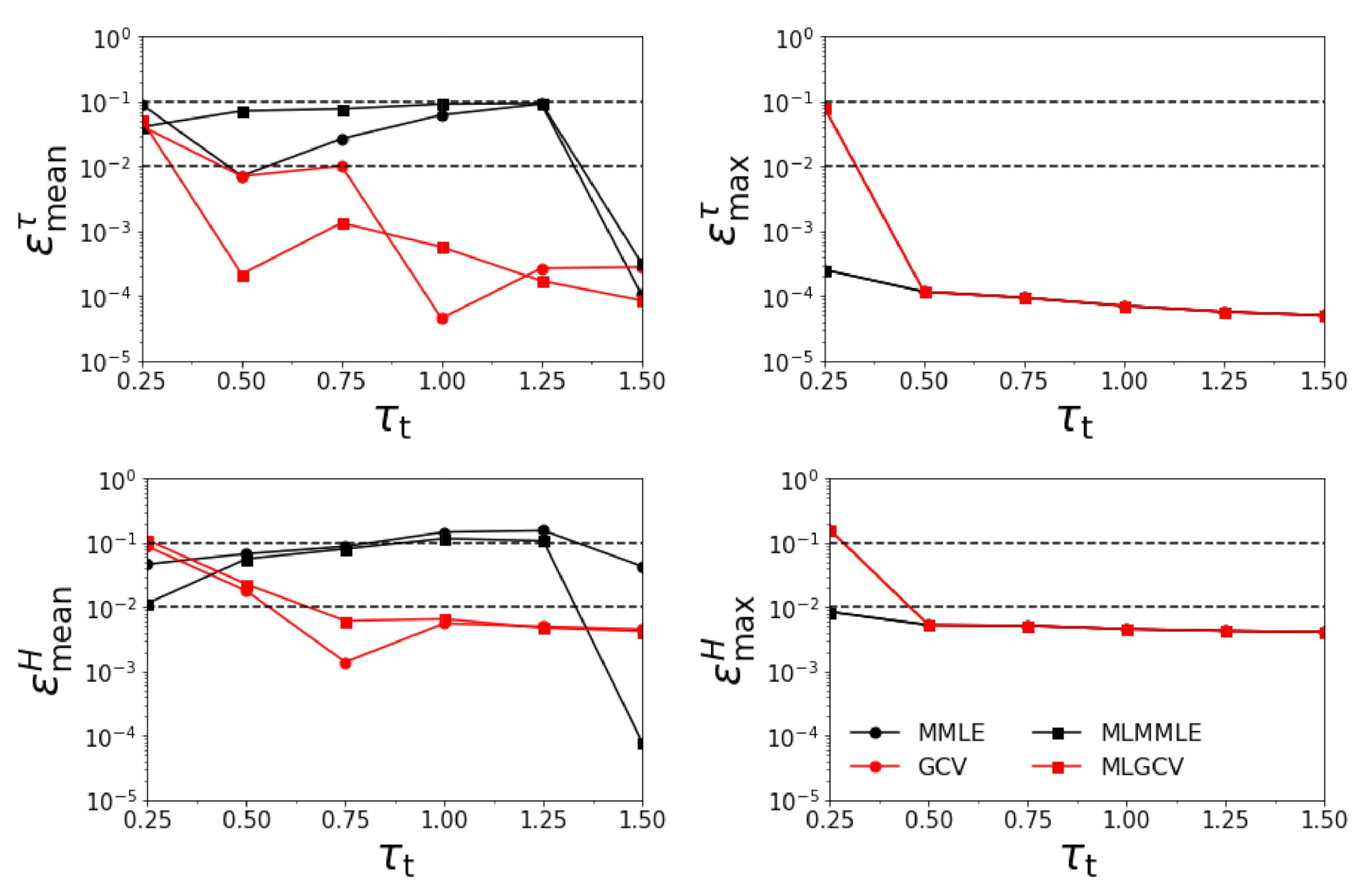
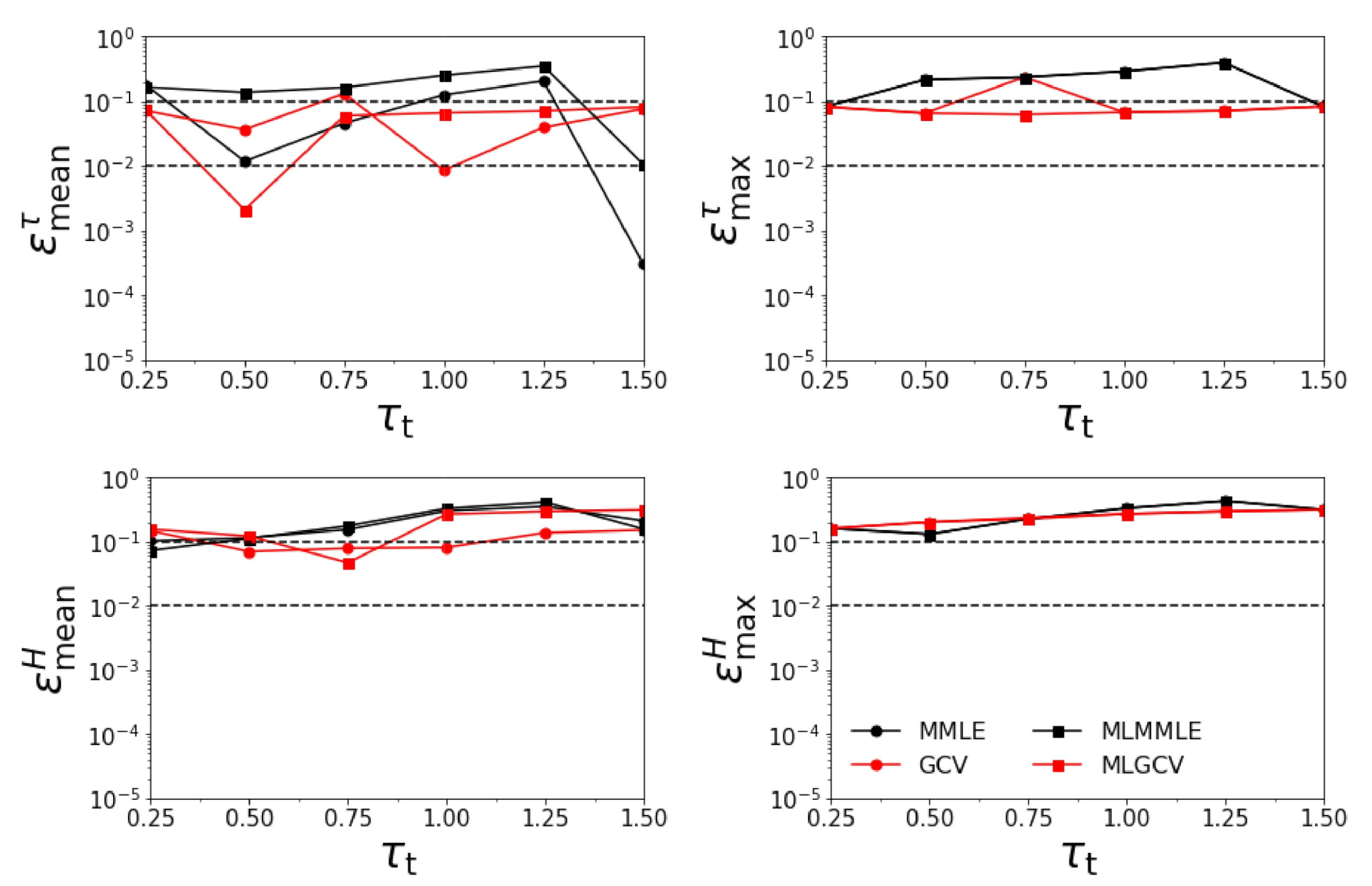
• Test Example 1

In the first example, we analyze the efficiency of the aerosol model selection by considering all models, i.e., we take m = 1, 2, 3, 4. Thus, the algorithm has the chance to identify the correct aerosol model. The solution accuracy is characterized by the relative errors:

$${\epsilon }_{\mathrm{mean}}^{\tau }=\frac{|{\tau }_{\mathrm{mean}}-{\tau }_{\mathrm{t}}|}{{\tau }_{\mathrm{t}}}\mathrm{and}{\epsilon }_{\mathrm{mean}}^H=\frac{|H_{\mathrm{mean}}-H_{\mathrm{t}}|}{{\tau }_{\mathrm{t}}}$$

corresponding to (cf. Equation (17)) ${\widehat{\mathbf{x}}}_{\mathrm{mean}}^{\delta }=[{\tau }_{\mathrm{mean}},H_{\mathrm{mean}}]$, and:

$${\epsilon }_{\max }^{\tau }=\frac{|{\tau }_{\max }-{\tau }_{\mathrm{t}}|}{{\tau }_{\mathrm{t}}}\mathrm{and}{\epsilon }_{\max }^H=\frac{|H_{\max }-H_{\mathrm{t}}|}{{\tau }_{\mathrm{t}}}$$

corresponding to (cf. Equation (15)) ${\widehat{\mathbf{x}}}_{\max }^{\delta }=[{\tau }_{\max },H_{\max }]$. In Figure 1 and Figure 2, we illustrate the variations of the relative errors with respect to ${\tau }_{\mathrm{t}}$ and $H_{\mathrm{t}}$, respectively, while in

Table 2. Average relative errors for the results plotted in Figure 1 and Figure 2. MMLE, Maximum Marginal Likelihood Estimation; GCV, Generalized-Cross Validation.

Method	Average Relative Error
	${\mathbf{\epsilon }}_{\mathrm{mean}\mathit{\tau }}^{\mathit{\tau }}$	${\mathbf{\epsilon }}_{\mathrm{mean}\mathit{\tau }}^{\mathit{H}}$	${\mathbf{\epsilon }}_{\mathrm{mean}\mathit{H}}^{\mathit{\tau }}$	${\mathbf{\epsilon }}_{\mathrm{mean}\mathit{H}}^{\mathit{H}}$
MMLE	0.046	0.091	0.027	0.102
MLMMLE	0.009	0.062	0.022	0.059
GCV	0.009	0.020	0.001	0.024
MLGCV	0.009	0.025	0.006	0.042

, we show the average relative errors:

$${\epsilon }_{\mathrm{mean}|\tau }^{\tau }=\frac{1}{N_{\tau }}\sum _{i=1}^{N_{\tau }}{\epsilon }_{\mathrm{mean}i}^{\tau }\mathrm{and}{\epsilon }_{\mathrm{mean}|\tau }^H=\frac{1}{N_{\tau }}\sum _{i=1}^{N_{\tau }}{\epsilon }_{\mathrm{mean}i}^H$$

over ${\tau }_{\mathrm{t}}$ for $N_{\tau }=6$, and:

$${\epsilon }_{\mathrm{mean}|H}^{\tau }=\frac{1}{N_H}\sum _{i=1}^{N_H}{\epsilon }_{\mathrm{mean}i}^{\tau }\mathrm{and}{\epsilon }_{\mathrm{mean}|H}^H=\frac{1}{N_H}\sum _{i=1}^{N_H}{\epsilon }_{\mathrm{mean}i}^H$$

over $H_{\mathrm{t}}$ for $N_H=5$. The following conclusions can be drawn:

• the relative errors ${\epsilon }_{\mathrm{mean}}^{\tau }$ and ${\epsilon }_{\mathrm{mean}}^H$ corresponding to the generalized cross-validation (GCV and MLGCV) are in general smaller than those corresponding to the maximum marginal likelihood estimation (MMLE and MLMMLE).
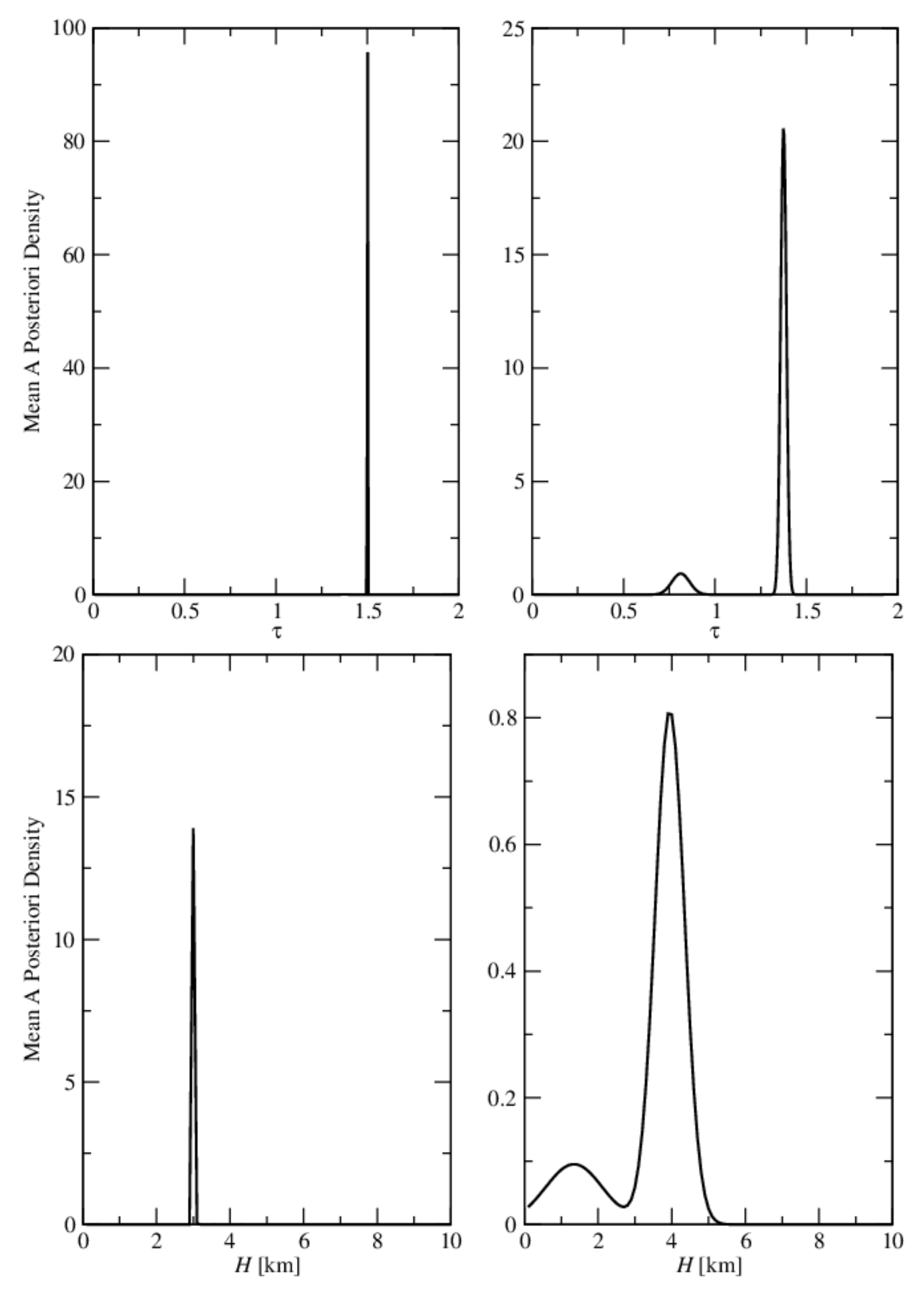
• the relative errors ${\epsilon }_{\max }^{\tau }$ and ${\epsilon }_{\max }^H$ are very small, and so, we deduce that the algorithm recognizes the exact aerosol model;
• the best method is GCV, in which case the average relative errors are ${\epsilon }_{\mathrm{mean}|\tau }^{\tau }=0.009$, ${\epsilon }_{\mathrm{mean}|\tau }^H=0.020$, ${\epsilon }_{\mathrm{mean}|H}^{\tau }=0.001$, and ${\epsilon }_{\mathrm{mean}|H}^H=0.024$;
• the aerosol optical thickness is better retrieved than the aerosol layer height.

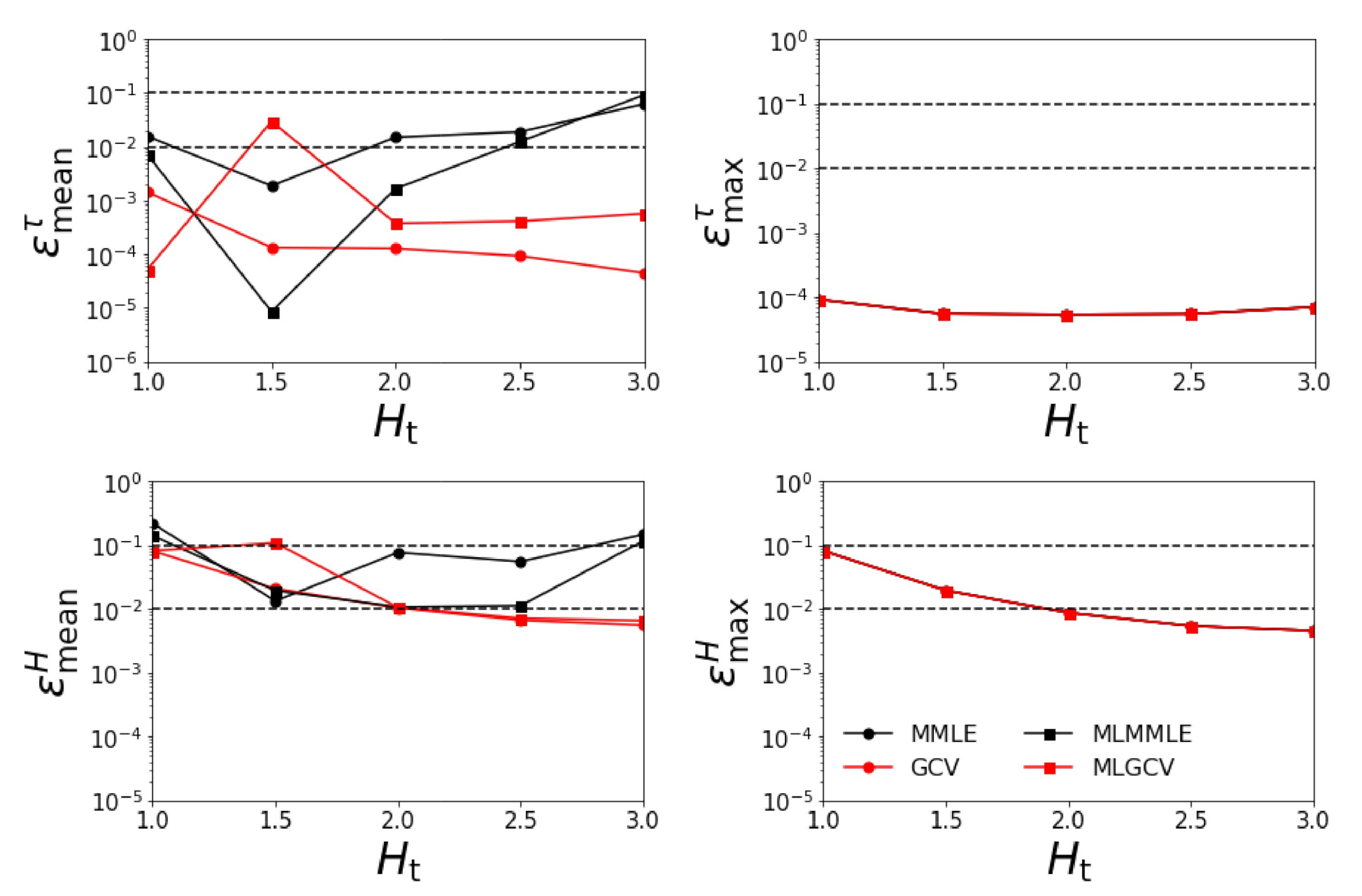
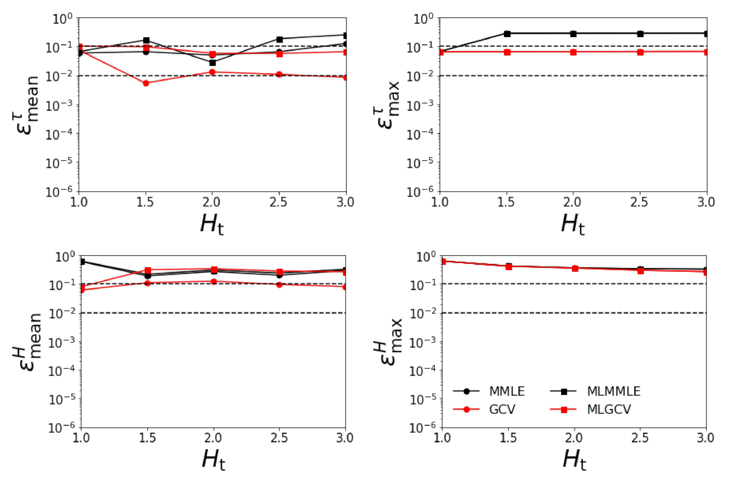
• Test Example 2

In the second example, we consider all aerosol models m except the exact one, i.e., we take $m=1,3,4$. In this more realistic scenario, the algorithm tries to find an aerosol model that is as close as possible to the exact one. The variations of the relative errors with respect to ${\tau }_{\mathrm{t}}$ and $H_{\mathrm{t}}$ are illustrated in Figure 3 and Figure 4, respectively, while the average relative errors are given in

Table 3. Average relative errors for the results plotted in Figure 3 and Figure 4.

Method	Average Relative Error
	${\mathbf{\epsilon }}_{\mathbf{mean}\mathit{\tau }}^{\mathit{\tau }}$	${\mathbf{\epsilon }}_{\mathbf{mean}\mathit{\tau }}^{\mathit{H}}$	${\mathbf{\epsilon }}_{\mathbf{mean}\mathit{H}}^{\mathit{\tau }}$	${\mathbf{\epsilon }}_{\mathbf{mean}\mathit{H}}^{\mathit{H}}$
MMLE	0.095	0.206	0.073	0.318
MLMMLE	0.180	0.210	0.139	0.348
GCV	0.060	0.111	0.022	0.096
MLGCV	0.059	0.200	0.076	0.259

. The following conclusions can be drawn:

• the relative errors ${\epsilon }_{\mathrm{mean}}^{\tau }$ and ${\epsilon }_{\mathrm{mean}}^H$ corresponding to the generalized cross-validation (GCV and MLGCV) are still smaller than those corresponding to the maximum marginal likelihood estimation (MMLE and MLMMLE).
• the relative errors ${\epsilon }_{\max }^{\tau }$ and ${\epsilon }_{\max }^H$ are extremely large, and so, we infer that the maximum solution estimate ${\widehat{\mathbf{x}}}_{\max }^{\delta }=[{\tau }_{\max },H_{\max }]$ is completely unrealistic;
• as before, the best method is GCV characterized by the average relative errors ${\epsilon }_{\mathrm{mean}|\tau }^{\tau }=0.060$, ${\epsilon }_{\mathrm{mean}|\tau }^H=0.111$, ${\epsilon }_{\mathrm{mean}|H}^{\tau }=0.022$, and ${\epsilon }_{\mathrm{mean}|H}^H=0.096$;
• the relative errors are significantly larger than those corresponding to the case when all four aerosol models are taken into account.

In Figure 5, we show the mean a posteriori density of $\tau$ and H computed by GCV for Test Examples 1 and 2. In Test Example 1, the a posteriori density is sharply peaked, indicating small errors in the retrieval, while in Test Example 2, the a posteriori density is wide and spread over all the aerosol models.

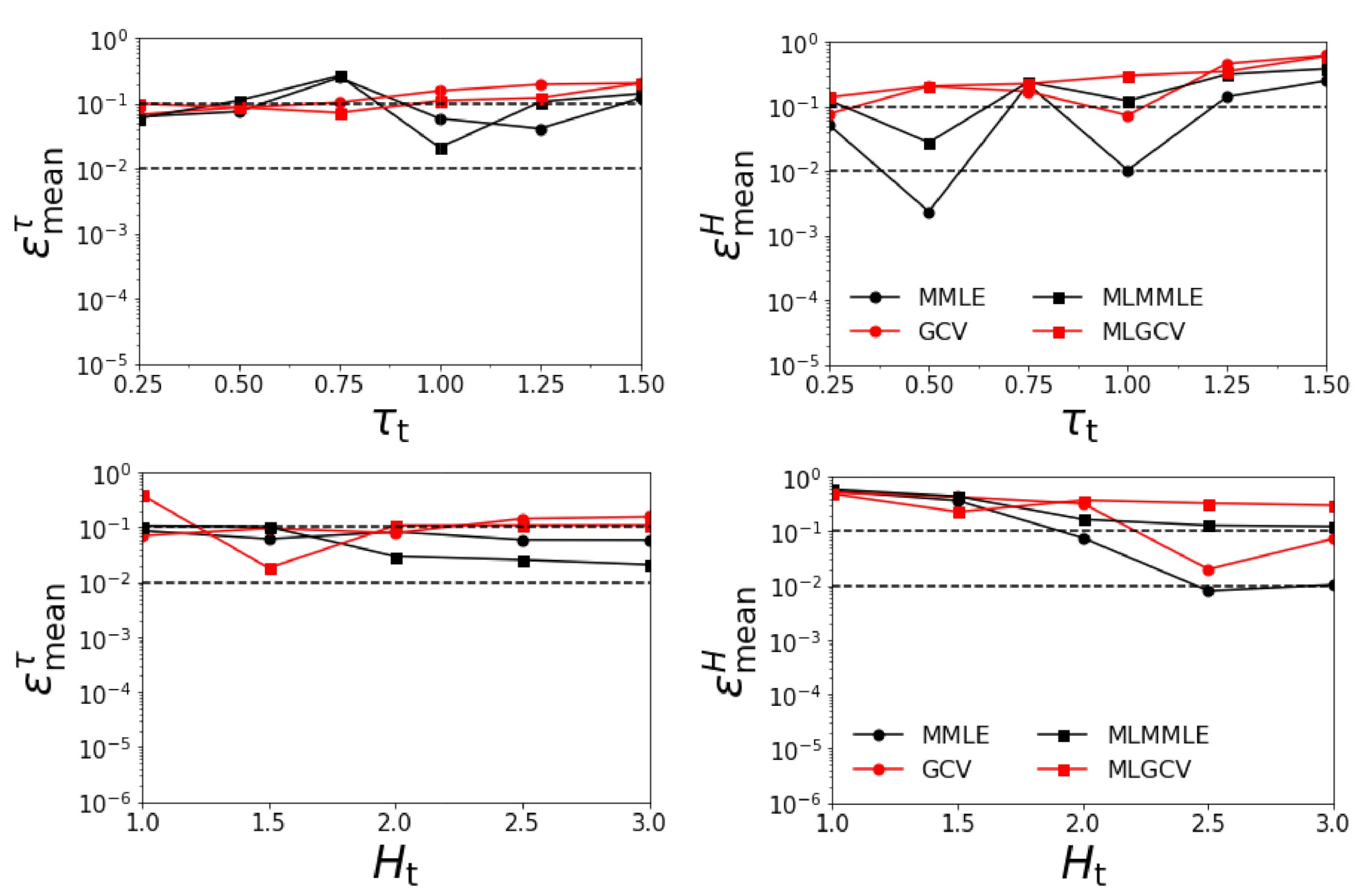
• Test Example 3

In the third series of our numerical experiments, we include the surface albedo in the retrieval. In fact, the surface albedo regarded as a model parameter can be (i) assumed to be known, (ii) included in the retrieval, or (iii) treated as a model uncertainty. The second situation, which leads to more accurate results, is considered here. In this case, however, the aerosol optical thickness and the surface albedo are strongly correlated (the condition number of ${\overline{\mathbf{K}}}_{mk}{\mathbf{L}}^{-1}$ at k = 1 is ${10}^3$–${10}^4$ times larger than for the case in which the surface albedo is not part of the retrieval). Since we are not interested in an accurate surface albedo retrieval, we chose the weight controlling the constraint of the surface albedo in the regularization matrix as $w_A={10}^3$. As $w_{\tau }=w_H=1.0$, this means that the surface albedo is tightly constrained to the a priori. We use the a priori and true values $A_{\mathrm{a}}=0.06$ and $A_{\mathrm{t}}=0.063$, respectively; thus, the uncertainty in the surface albedo with respect to the a priori is 5%. The synthetic measurements are generated with the true surface albedo of 0.063.

In Figure 6, we illustrate the variations of the relative errors ${\epsilon }_{\mathrm{mean}}^{\tau }$ and ${\epsilon }_{\mathrm{mean}}^H$ with respect to ${\tau }_{\mathrm{t}}$ and $H_{\mathrm{t}}$, when all four aerosol models are taken into account. The average relative errors are given in

Table 4. Average relative errors for the results plotted in Figure 6.

Method	Average Relative Error
	${\mathbf{\epsilon }}_{\mathbf{mean}\mathit{\tau }}^{\mathit{\tau }}$	${\mathbf{\epsilon }}_{\mathbf{mean}\mathit{\tau }}^{\mathit{H}}$	${\mathbf{\epsilon }}_{\mathbf{mean}\mathit{H}}^{\mathit{\tau }}$	${\mathbf{\epsilon }}_{\mathbf{mean}\mathit{H}}^{\mathit{H}}$
MMLE	0.042	0.046	0.018	0.042
MLMMLE	0.051	0.060	0.011	0.027
GCV	0.101	0.213	0.076	0.237
MLGCV	0.119	0.311	0.100	0.398

. The results show that:

• the relative errors ${\epsilon }_{\mathrm{mean}}^{\tau }$ and ${\epsilon }_{\mathrm{mean}}^H$ corresponding to generalized cross-validation (GCV and MLGCV) are in general larger than those corresponding to maximum marginal likelihood estimation (MMLE and MLMMLE);
• the best methods are MMLE and MLMMLE; the average relative errors given by MLMMLE are ${\epsilon }_{\mathrm{mean}|\tau }^{\tau }=0.051$, ${\epsilon }_{\mathrm{mean}|\tau }^H=0.060$, ${\epsilon }_{\mathrm{mean}|H}^{\tau }=0.011$, and ${\epsilon }_{\mathrm{mean}|H}^H=0.027$;
• the relative errors are significantly larger than those obtained in the first two test examples (when the surface albedo is known exactly).

Figure 7 illustrates the variations of the relative errors ${\epsilon }_{\mathrm{mean}}^{\tau }$ and ${\epsilon }_{\mathrm{mean}}^H$ with respect to ${\tau }_{\mathrm{t}}$ and $H_{\mathrm{t}}$, when all aerosol models except the exact one are considered. The corresponding average relative errors are given in

Table 5. Average relative errors for the results plotted in Figure 7.

Method	Average Relative Error
	${\mathbf{\epsilon }}_{\mathbf{mean}\mathit{\tau }}^{\mathit{\tau }}$	${\mathbf{\epsilon }}_{\mathbf{mean}\mathit{\tau }}^{\mathit{H}}$	${\mathbf{\epsilon }}_{\mathbf{mean}\mathit{H}}^{\mathit{\tau }}$	${\mathbf{\epsilon }}_{\mathbf{mean}\mathit{H}}^{\mathit{H}}$
MMLE	0.101	0.113	0.070	0.204
MLMMLE	0.117	0.203	0.057	0.291
GCV	0.136	0.269	0.109	0.274
MLGCV	0.116	0.307	0.147	0.346

. The results show that:

• as in the previous scenario, the relative errors ${\epsilon }_{\mathrm{mean}}^{\tau }$ and ${\epsilon }_{\mathrm{mean}}^H$ corresponding to generalized cross-validation (GCV and MLGCV) are in general larger than those corresponding to maximum marginal likelihood estimation (MMLE and MLMMLE).
• the best methods are MMLE and MLMMLE; the average relative errors delivered by MMLE are ${\epsilon }_{\mathrm{mean}|\tau }^{\tau }$ = 0.101, ${\epsilon }_{\mathrm{mean}|\tau }^H$ = 0.113, ${\epsilon }_{\mathrm{mean}|H}^{\tau }$ = 0.070, and ${\epsilon }_{\mathrm{mean}|H}^H$ = 0.204;
• the relative errors are the largest among all the test examples.

8. Conclusions

We designed a retrieval algorithm that takes into account uncertainty in model selection. The solution corresponding to a specific model is characterized by a metric called relative evidence, which is a measure of the fit between the model and the measurement. Based on this metric, the maximum solution estimate, corresponding to the model with the highest evidence, and the mean solution estimate, representing a linear combination of solutions weighted by their evidence, are introduced.

The retrieval algorithm is based on:

• an application of the prewhitening technique in order to transform the data model into a scaled model with white noise;
• a deterministic regularization method, i.e., the iteratively regularized Gauss–Newton method, in order to compute the regularized solution (equivalent to the maximum a posteriori estimate of the solution in a Bayesian framework) and to determine the optimal value of the regularization parameter (equivalent to the ratio of the data error and a priori state variances in a Bayesian framework);
• a linearization of the forward model around the solution in order to transform the nonlinear data model into a linear model and, in turn, facilitate an analytical integration of the likelihood density over the state vector;
• an extension of maximum marginal likelihood estimation and generalized cross-validation to model selection and data error variance estimation.

Essentially, the algorithm includes four selection models corresponding to:

• the two parameter choice methods used (maximum marginal likelihood estimation and generalized cross-validation) and
• the two settings in which the relative evidence is treated (stochastic and deterministic).

The algorithm is applied to the retrieval of aerosol optical thickness and aerosol layer height from synthetic measurements corresponding to the EPIC instrument. In the simulations, the aerosol models implemented in the MODIS aerosol algorithm over land are considered, and the surface albedo is either assumed to be known or included in the retrieval. The following conclusions are drawn:

• The differences between the results corresponding to the stochastic and deterministic interpretations of the relative evidence are not significant.
• If the surface albedo is assumed to be known, generalized cross-validation is superior to maximum marginal likelihood estimation; if the surface albedo is included in the retrieval, the contrary is true.
• The errors in the aerosol optical thickness retrieval are smaller than those in the aerosol layer height retrieval. In the most realistic situation, when the exact aerosol model and surface albedo are unknown, the average relative errors in the retrieved aerosol optical thickness are about 10%, while the corresponding errors in the aerosol layer height are about 20%.
• The maximum solution estimate is completely unrealistic when both the aerosol model and surface albedo are unknown.

References

- Levy, R.C.; Remer, L.A.; Dubovik, O. Global aerosol optical properties and application to Moderate Resolution Imaging Spectroradiometer aerosol retrieval over land. J. Geophys. Res. Atmos. 2007, 112. [Google Scholar] [CrossRef]
- Hoeting, J.A.; Madigan, D.; Raftery, A.E.; Volinsky, C.T. Bayesian Model averaging: A tutorial. Stat. Sci. 1999, 14, 382–401. [Google Scholar]
- Määttä, A.; Laine, M.; Tamminen, J.; Veefkind, J. Quantification of uncertainty in aerosol optical thickness retrieval arising from aerosol microphysical model and other sources, applied to Ozone Monitoring Instrument (OMI) measurements. Atmos. Meas. Tech. 2014, 7, 1185–1199. [Google Scholar] [CrossRef]
- Kauppi, A.; Kolmonen, P.; Laine, M.; Tamminen, J. Aerosol-type retrieval and uncertainty quantification from OMI data. Atmos. Meas. Tech. 2017, 10, 4079–4098. [Google Scholar] [CrossRef]
- Doicu, A.; Trautmann, T.; Schreier, F. Numerical Regularization for Atmospheric Inverse Problems; Springer: Berlin/Heidelberg, Germany, 2010. [Google Scholar] [CrossRef]
- Tarantola, A. Inverse Problem Theory and Methods for Model Parameter Estimation; Society for Industrial and Applied Mathematics (SIAM): Philadelphia, PA, USA, 2005. [Google Scholar] [CrossRef]
- Patterson, H.; Thompson, R. Recovery of inter-block information when block sizes are unequal. Biometrika 1971, 58, 545–554. [Google Scholar] [CrossRef]
- Smyth, G.K.; Verbyla, A.P. A conditional likelihood approach to residual maximum likelihood estimation in generalized linear models. J. R. Stat. Soc. Ser. Methodol. 1996, 58, 565–572. [Google Scholar] [CrossRef]
- Stuart, A.; Ord, J.; Arnols, S. Kendall’s Advanced Theory of Statistics. Volume 2A: Classical Inference and the Linear Model; Oxford University Press Inc.: Oxford, UK, 1999. [Google Scholar]
- Wahba, G. Practical approximate solutions to linear operator equations when the data are noisy. SIAM J. Numer. Anal. 1977, 14, 651–667. [Google Scholar] [CrossRef]
- Wahba, G. Spline Models for Observational Data; Society for Industrial and Applied Mathematics (SIAM): Philadelphia, PA, USA, 1990. [Google Scholar] [CrossRef]
- Marshak, A.; Herman, J.; Szabo, A.; Blank, K.; Carn, S.; Cede, A.; Geogdzhayev, I.; Huang, D.; Huang, L.K.; Knyazikhin, Y.; et al. Earth Observations from DSCOVR EPIC Instrument. Bull. Am. Meteorol. Soc. 2018, 99, 1829–1850. [Google Scholar] [CrossRef] [PubMed]
- Geogdzhayev, I.V.; Marshak, A. Calibration of the DSCOVR EPIC visible and NIR channels using MODIS Terra and Aqua data and EPIC lunar observations. Atmos. Meas. Tech. 2018, 11, 359–368. [Google Scholar] [CrossRef] [PubMed]
- Xu, X.; Wang, J.; Wang, Y.; Zeng, J.; Torres, O.; Reid, J.; Miller, S.; Martins, J.; Remer, L. Detecting layer height of smoke aerosols over vegetated land and water surfaces via oxygen absorption bands: Hourly results from EPIC/DSCOVR in deep space. Atmos. Meas. Tech. 2019, 12, 3269–3288. [Google Scholar] [CrossRef]
- García, V.M.; Sasi, S.; Efremenko, D.S.; Doicu, A.; Loyola, D. Radiative transfer models for retrieval of cloud parameters from EPIC/DSCOVR measurements. J. Quant. Spectrosc. Radiat. Transf. 2018, 213, 228–240. [Google Scholar] [CrossRef]
- García, V.M.; Sasi, S.; Efremenko, D.S.; Doicu, A.; Loyola, D. Linearized radiative transfer models for retrieval of cloud parameters from EPIC/DSCOVR measurements. J. Quant. Spectrosc. Radiat. Transf. 2018, 213, 241–251. [Google Scholar] [CrossRef]
- Holben, B.; Eck, T.; Slutsker, I.; Tanré, D.; Buis, J.; Setzer, A.; Vermote, E.; Reagan, J.; Kaufman, Y.; Nakajima, T.; et al. AERONET—A federated instrument network and data archive for aerosol characterization. Remote Sens. Environ. 1998, 66, 1–16. [Google Scholar] [CrossRef]