Classification of the Complex Agricultural Planting Structure with a Semi-Supervised Extreme Learning Machine Framework

Abstract

Many approaches have been developed to analyze remote sensing images. However, for the classification of large-scale problems, most algorithms showed low computational efficiency and low accuracy. In this paper, the newly developed semi-supervised extreme learning machine (SS-ELM) framework with k-means clustering algorithm for image segmentation and co-training algorithm to enlarge the sample sets was used to classify the agricultural planting structure at large-scale areas. Data sets collected from a small-scale area within the Hetao Irrigation District (HID) at the upper reaches of the Yellow River basin were used to evaluate the SS-ELM framework. The results of the SS-ELM algorithm were compared with those of the random forest (RF), ELM, support vector machine (SVM) and semi-supervised support vector machine (S-SVM) algorithms. Then the SS-ELM algorithm was applied to analyze the complex planting structure of HID in 1986–2010 by comparing the remote sensing estimated results with the statistical data. In the small-scale case, the SS-ELM algorithm performed better than the RF, ELM, SVM, and S-SVM algorithms. For the SS-ELM algorithm, the average overall accuracy (OA) was in a range of 83.00–92.17%. On the contrary, for the other four algorithms, their average OA values ranged from 56.97% to 92.84%. Whereas, in the classification of planting structure in HID, the SS-ELM algorithm had an excellent performance in classification accuracy and computational efficiency for three major planting crops including maize, wheat, and sunflowers. The estimated areas by using the SS-ELM algorithm based on the remote sensing images were consistent with the statistical data, and their difference was within a range of 3–25%. This implied that the SS-ELM framework could be served as an effective method for the classification of complex planting structures with relatively fast training, good generalization, universal approximation capability, and reasonable learning accuracy.

1. Introduction

The remote sensing image data provides material for the detailed interpretation of large-scale surface coverage [1,2]. Based on the remote sensing data and combined with the current classification and recognition algorithms of surface features, an effective inversion of surface coverage can be achieved to some extent [3,4,5]. Among them, the effective classification of surface vegetation can provide key basic information for identifying surface cover types and plant growth conditions over large scales and estimating regional evapotranspiration. All of the data are significant for regional crop management, crop yield estimation, and the protection of agroecosystems. For the classification of large-scale agricultural planting structure, the traditional manual investigation method is time-consuming, labor-intensive, and consumes an abundance of resources. The recently developed machine learning methods, i.e. decision trees, feature extraction, neural networks, SVM, etc., provide promising tools. However, the low resolution of early remote sensing data before 2000 is a big challenge for manually extracting reasonable samples, and the machine learning algorithms are not able to obtain reasonable results from huge amounts of data within a certain period. The algorithm of combining semi-supervised learning with the ELM is supposed to be useful to the classification of large-scale agricultural planting structure.

Recently, land-use scene classification by remote sensing image technology with classification algorithms [3,6] has attracted more attention for its broad application prospects in regional management. Satellite remote sensing [7,8] and unmanned aerial vehicles (UAVs) [4,9] image acquisition technologies are two typical ways, which have been widely applied in geology, hydrology, agriculture, and forestry and environmental monitoring, etc. Satellite remote sensing has made it possible to obtain large-area images efficiently. To make better use of the remote sensing image data, a variety of classification algorithms have been developed and applied to obtain the required information. In general, the classification algorithm is a significant information acquisition technique for hyperspectral imagery, which focuses on distinguishing physical objects.

The random forest (RF) [2,10], extreme-learning machine (ELM) [3,11,12], and the support vector machine (SVM) [13,14,15] have been widely applied due to their remarkable performance in remote sensing image classification. The semi-supervised extreme learning machine (SS-ELM) algorithm has been used in the detection of the industrial aluminum production cell and the optic disc [16,17]. They designed a semi-supervised based ELM algorithm which incorporates the graph Laplacian and ELM into a unified framework for handling the classification problem of a small number of labelled samples. With this SS-ELM method, the overall classification accuracy of the industrial and medical images was improved significantly [16,18]. However, it is unlikely for the SS-ELM with the graph Laplacian to construct a reasonable graph due to the low resolution of the remote sensing images and the amount of huge data in large-scale agricultural planting areas.

Most previous research focus on using supervised methods on a relatively small-scale or low-level images classification basis. For a large-scale region, it usually shows a complex pixel structure with multiple land cover types. The traditional supervised classification methods may encounter the problems of low classification accuracy and/or low computational efficiency, due to an insufficiently labeled sample set. Therefore, a more efficient algorithm with enlarged sample sets has become extremely pertinent. The semi-supervised learning (SSL) algorithm is an effective approach to overcome the problem of small-size labeled samples in high-dimensional data classification. The SSL algorithm can be divided into five types, i.e., (1) generative model [19], (2) self-training [20], (3) co-training [21], (4) transductive support vector machine (TSVM) [22], and (5) graph-based method [23]. The self-training and co-training algorithms have been widely used for acquiring enlarged sample datasets. The self-training algorithm uses the previous classification results to train the classifier iteratively. The co-training algorithm trains two classifiers with the labeled samples in two independent subsets. It selects the unlabeled samples with high reliability to train the other classifier separately. The SSL algorithm has been used in land cover or land use classification. For example, a self-training method was proposed using the support vector machine (SVM) based supervised learner and the minimum spanning tree (MST) based graph clustering, and it performed well in land-cover classification [24]. However, using the SSL algorithm still cannot obtain a large number of labeled samples for classifying large-scale agricultural planting structure and forest resources. The limited labeled samples may reduce the training accuracy of the algorithm. Moreover, it is a laborious task to train an effective classifier.

To our knowledge, using the SS-ELM framework for regional ground object recognition has not been well studied. Therefore, the objectives of the present research are (1) to evaluate the performance in accuracy and effectiveness of the SS-ELM algorithm compared with traditional classification algorithms using the visual interpretation data of a small-scale area with complex planting structures under different labeled sample sizes, and (2) to apply the SS-ELM algorithm in a large-scale agricultural area with Landsat images to obtain highly accurate vegetation recognition.

2. Research Area and Data

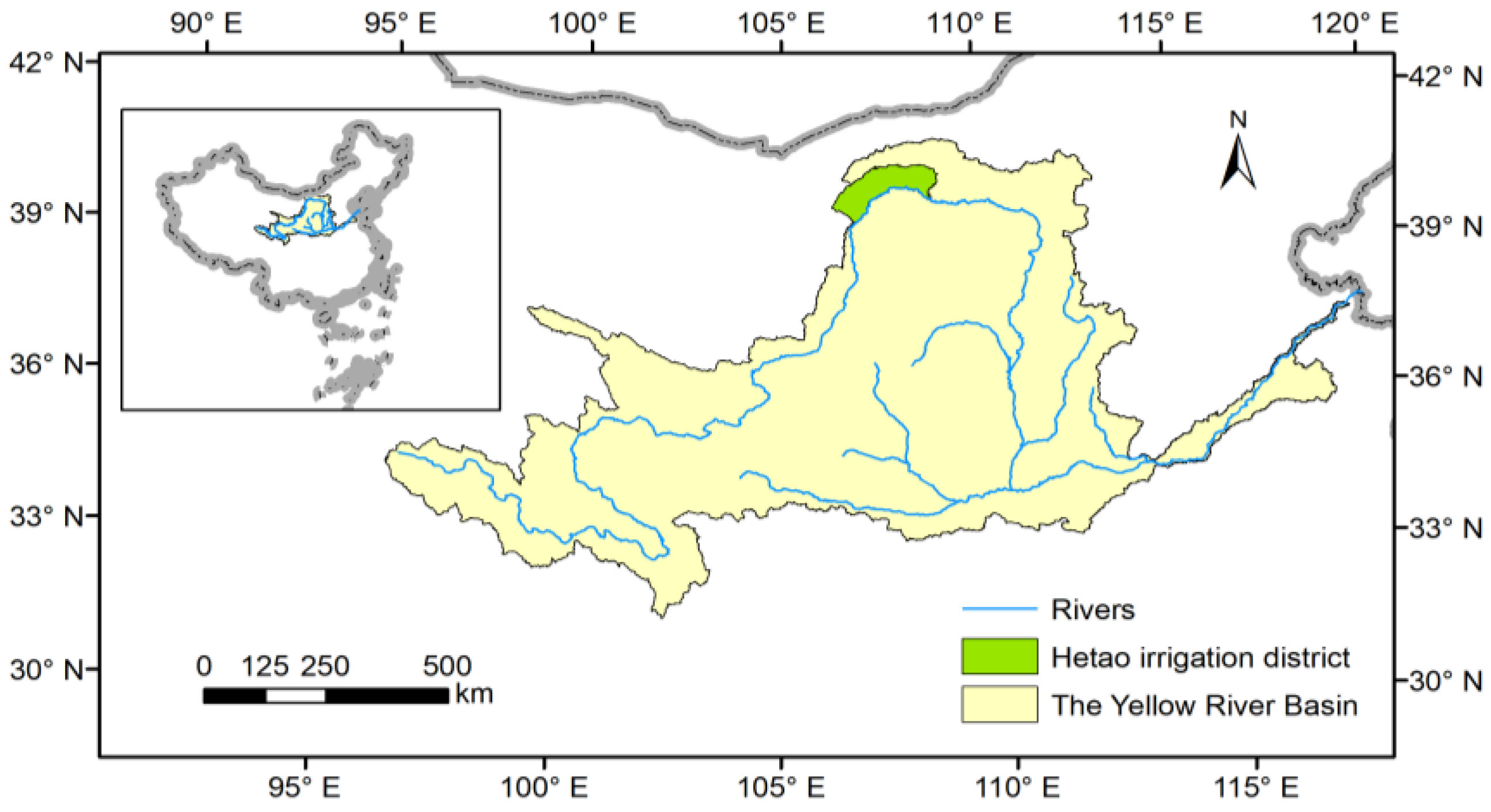
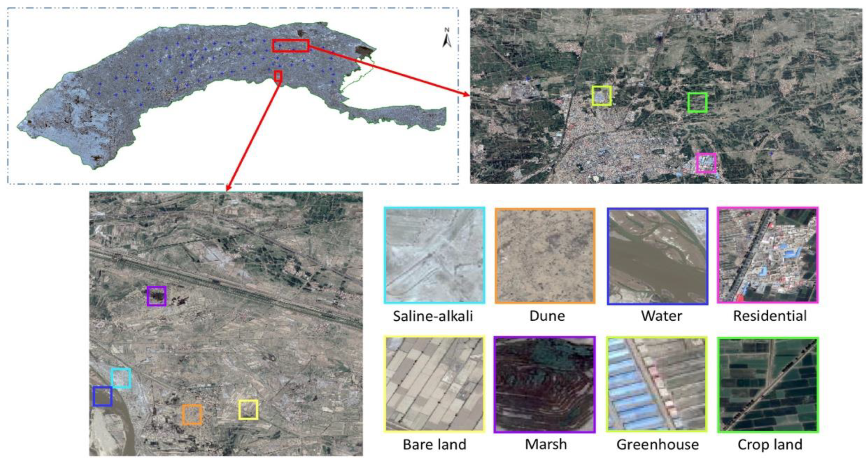
2.1. Research Area

The Hetao irrigation district (HID) located in the upper reaches of the Yellow River basin (latitude 40.1°N–41.4°N, longitude 106.1°N–109.4°E) was selected as the study area (see Figure 1). HID covers an area of 1.12 Mha, in which about 570,000 ha is irrigated farmland.

As shown in Figure 2, the land-use categories can be further classified as saline–alkali land, sand dune, waterbody, residential area, bare land, marsh, greenhouse, and cropland. All these land use categories had been segmented before the classification of cropping areas in Section 3.1. Maize, spring wheat, sunflowers, and horticulture crops, e.g., watermelons, tomatoes and peppers are the main crops grown in HID recently. The growing season of spring wheat begins in late March and ends in mid-July. The maize growing season is from late April to late September. Sunflowers and vegetables are both planted in late May and harvested in mid-September and late August, respectively. Meanwhile, the landscape is often divided into small farms with fragmented cropping patterns due to the smallholder policy of the farmland use rights.

2.2. Data and Preprocessing

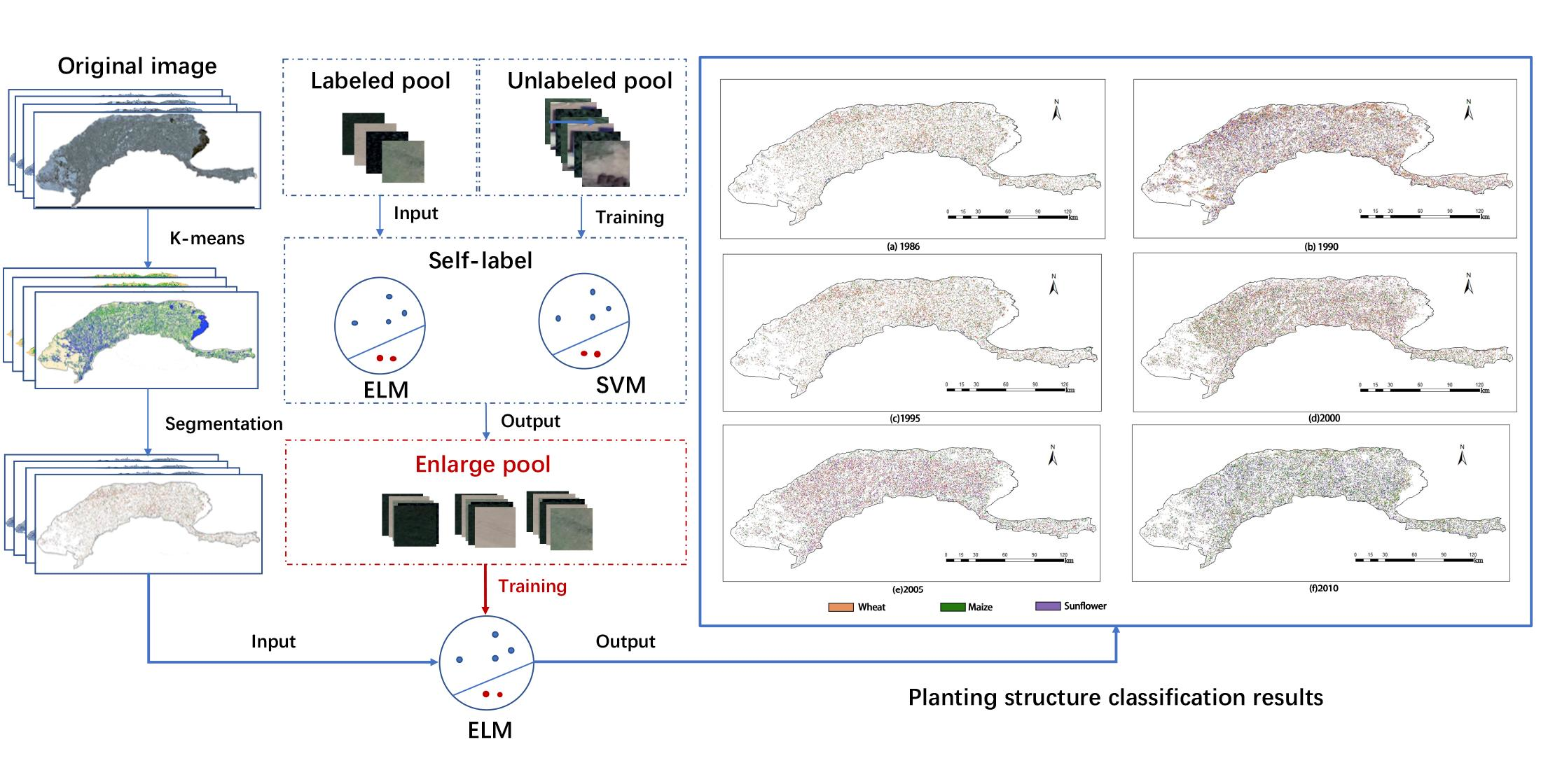
Twenty-four Landsat Thematic Mapper (TM) and Operational Land Imager (OLI) images covering HID from 1986 to 2010 (see

Table 1. Description of the 24 Landsat Thematic Mapper (TM) and Operational Land Imager (OLI) images of the study area (HID).

Year and Data Source	HID			Year and Data Source	HID
	Path/Row	Date	Cloud%		Path/row	Date	Cloud%
1986 Landsat TM	128/31	1986.08.09	1	2000 Landsat OLI	128/31	2000.09.24	0
	128/32	1986.08.09	0		128/32	2000.09.08	0
	129/31	1986.07.31	6		129/31	2000.09.24	0
	129/32	1986.07.31	1		129/32	2000.08.30	5.09
1990 Landsat TM	128/31	1990.09.05	9	2005 Landsat OLI	128/31	2005.10.24	0.07
	128/32	1990.06.01	0		128/32	2005.10.08	0.23
	129/31	1990.08.11	0		129/31	2005.09.13	0.02
	129/32	1990.07.10	1.69		129/32	2005.09.13	0.05
1995 Landsat TM	128/31	1995.09.19	0	2010 Landsat OLI	128/31	2010.08.19	0
	128/32	1995.09.19	0		128/32	2010.08.19	0.1
	129/31	1995.09.10	0.27		129/31	2010.08.26	0.19
	129/32	1995.09.26	0		129/32	2010.09.11	0

Note: HID represents the Hetao Irrigation District.

) were downloaded from https://earthexplorer.usgs.gov/. These images have six (for TM) or eight (for OLI) multispectral bands with the spatial resolution of 30 m × 30 m and one panchromatic band with the resolution of 15 m × 15 m. The L1T-level Landsat images (TM and OLI) were geometrically corrected by the system up to sub-pixel accuracy without further geometric correction. To obtain consistently geometrical data (TM and OLI) from different sensors, the relative radiation was normalized based on the enhanced thematic mapper plus (ETM+) images, and the normalization was carried out for OLI images in 2000–2010. Table 1 describes the 24 Landsat Thematic Mapper (TM) and Operational Land Imager (OLI) images used in this study. In the small-scale test case, the Google Earth’s historical images with a spatial resolution of 1.6 m were used to improve the fitting accuracy.

The statistical data of the planting area of the three crops from 1986 to 2010 are available at the Bayannur Agricultural Information Network (http://www.bmagri.gov.cn), Bayannur Statistics Bureau (http://tjj.bynr.gov.cn), and the Administration Bureau of the Hetao Irrigation District (http://www.zghtgq.com/).

The software ENVI 5.4 was employed for pre-processing the downloaded Landsat TM/OLI images, the preprocess includes band combination, atmospheric correction with the fast line-of-sight-atmospheric analysis of spectral hypercubes (FLAASH) tool, image mosaic, and image subset. The purpose of atmospheric correction is to eliminate the influence of atmosphere and illumination on the reflectance of ground objects and to obtain near-surface reflectance.

3. Methodology

To improve the accuracy and efficiency of the traditional supervised learning-based classification, a newly developed semi-supervised extreme learning machine (SS-ELM) classification method, which combines image segmentation with a new self-label algorithm, was used in the following classification. The classification method includes three steps: image segmentation with k-means, self-label, and planting structure classification (see Figure 3). First, the non-agricultural regions are segmented using k-means unsupervised learning algorithm. Then the co-training self-label algorithm based on the SVM and ELM classifiers is used to enlarge the sample set (see

Table 2. The procedure of the co-training self-label algorithm (CTSLAL).

1:	Input: labeled set L, unlabeled set U
2:	Output: enlarged set EL
3:	initializeEL = L; co-training labeled set CL as empty;
4:	clf_svm; clf_elm the independent classifiers are initially trained with L
5:	while length (EL) increases do processes the CL set until the sample number of EL doesn’t change
6:	clf_svm; clf_elm; update training (clf_svm; clf_elm; EL+L)
7:	Co_labeling (clf_svm; clf_elm; EL; CL)
8:	end while
9:	ReturnEL

). Finally, the enlarged sample set is used to perform the classification of agricultural planting structure in the large-scale area.

3.1. Image Segmentation with k-Means

The k-means clustering algorithm, also known as a kind of semi-supervised learning which is simple and fast. It is based on an iterative process that divides the image into different clusters [25,26,27]. The data points or pixels are grouped exclusively. In this case, if a data point belongs to a certain cluster, then it will not belong to any other clusters. Conventional k-means clustering is selected where the clusters are fully dependent on the selection of the initial centroid point [28,29]. The k-means algorithm assumes Euclidean distance based on the similarity and/or dissimilarity. The Euclidean distance of the k-means algorithm can be expressed as

$$D=\sqrt{{\displaystyle \sum }_{k=1}^n{\left(p_k-q_k\right)}^2}$$

(1)

where D is the Euclidean distance of the k-means algorithm, p_k and q_k are the k-th the pixel intensity of data objects p and q, respectively, and n is the number of clusters. Initial seed points for the k-means clustering are randomly chosen for the entire image, and the distances between all the pixels and seed points are calculated. Pixels with minimum distance to the respective seed point are clustered together. A new mean value is calculated in each iteration. The interaction continues until there is no change or variation in the mean value.

In this study, different k values have been tested, and a stable clustering result can be obtained for k = 25. Thus, 25 clusters are selected for the k-means segmentation. The pixels of each region in the segmented image is statistically analyzed. After that, the adjacent clusters of non-agricultural regions are combined, and then further image segmentation is performed.

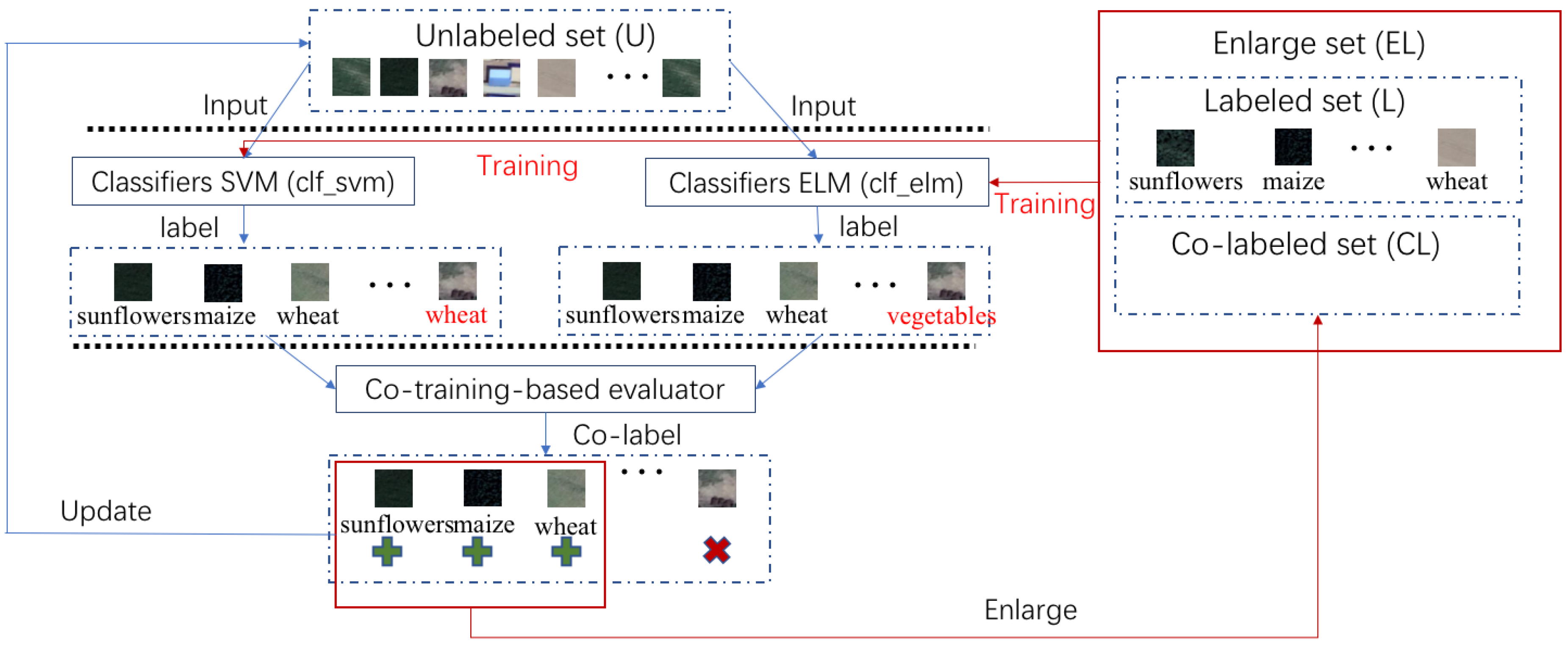
3.2. The Co-Training Self-Label Method

3.2.1. The ELM

The ELM has been widely adopted for various classifications, with its significant advantage of extremely fast training, learning accuracy, and good generalization [30]. The standard ELM has the structure of single-hidden layer feed-forward neural networks (SLFNs) [30], which contains input layer, hidden layer, and output layer. Implementing the ELM includes two steps, the first is to transform the input data into the hidden layer by using the ELM feature mapping, and the second step is to generate the results by using the ELM learning.

The relationship between output and input of the SLFNs with L hidden nodes can be expressed as follows:

$$f\left(x\right)=h\left(x\right)\beta ={\displaystyle \sum }_{i=1}^L{h}_i\left(x\right)\ast {\beta }_i={\displaystyle \sum }_{i=1}^L{G}_i\left(x,c_i,b_i\right)\ast {\beta }_i$$

(2)

where f (•) is the output of the neural network, x is the input of neural networks, β_i = [β₁, …, β_L]^T is the vector of the output weights between the hidden layer with L nodes to the output layer with m nodes, h(x) = [h₁(x), …, h_L(x)] is the output vector of the hidden layer, G_i(•) is the i-th hidden node activation function, c_i is the input weight vector connecting the input layer to the i-th hidden layer, and b_i is the bias weight of the i-th hidden layer. The different hidden neurons can adopt different activation functions, e.g., Fourier function, hard-limit function, and Gaussian function [31,32,33].

If different activation functions are selected, the resulting expressions are different. In this study, the following activation function was used:

$$G\left(x,c_i,b_i\right)=g\left(c_{i}x+b_i\right)$$

(3)

Different from the traditional learning algorithms, the ELM emphasizes that the hidden neurons should be fixed, and the ELM solutions aim to find the smallest training error and the smallest norm of output weights [33]:

$$Minimize:{\parallel \beta \parallel }_{s_1}^{{\sigma }_1}+C{\parallel H\beta -T\parallel }_{s_2}^{{\sigma }_2}$$

(4)

where σ₁ > 0, σ₂ > 0, s₁, s₂ = 0, 1/2, 1, 2, …, +∞. H is the hidden layer output matrix, which can be written as

$$H=\left[\begin{array}{c}h\left(x_1\right)\\ ⋮\\ h\left(x_n\right)\end{array}\right]=\left[\begin{array}{ccc}{h}_1\left(x_1\right)& \dots & h_L\left(x_1\right)\\ ⋮& \dots & \dots \\ h_1\left(x_n\right)& \cdots & h_L\left(x_n\right)\end{array}\right]$$

(5)

and n is the number of input nodes, m is the number of output nodes. T is the training data-target matrix, which can be expressed as

$$T=\left[\begin{array}{c}{t}_1^T\\ ⋮\\ t_n^T\end{array}\right]=\left[\begin{array}{ccc}{t}_{11}& \dots & t_{1m}\\ ⋮& \dots & \dots \\ t_{n1}& \cdots & t_{nm}\end{array}\right]$$

(6)

The output weight β is calculated by the following equation:

$$\widehat{\beta }=H^{†}T$$

(7)

where $H^{†}$ is the Moore–Penrose generalized inverse of matrix H.

With the aforementioned descriptions, fast and effective learning can be established. Given a training set,

Y = {(y_i, t_i)|y_i ∈ Rⁿ, t_i ∈ R^m, i = 1, …, n}

(8)

where Y is the training set, y_i is the training data which is the value of each band of an image pixel, and t_i is the class label of each sample, e.g., the label of vegetables, maize, wheat, and sunflowers, etc.

The flowchart of the ELM can be found in Figure 4, and the calculated process of the ELM training algorithm can be summarized as follows [33]:

• Randomly assign the hidden node parameters: the input weights c_i and biases b_i.
• Calculate output matrix H of the hidden layer with Equation (5).
• Obtain the output weight β with Equation (7).

3.2.2. The Co-Training Self-Label Algorithm

The co-training self-label algorithm (CTSLAL) is an effective solution for learning a significant number of unlabeled samples and obtaining sufficient training datasets for fully supervised learning. The detailed procedure of the CTSLAL is presented in Figure 5 and Table 2. The CTSLAL includes two main processes: training and labeling. In the training process, the labeled set is used as the initial training set to create the SVM and ELM classifier. Then, the enlarged labeled set is used as the training set to update the SVM and ELM classifiers. In the labeling stage, a proportion of unlabeled samples are fed to the pre-trained SVM and ELM classifiers to output the confidence in each category. The CTSLAL combines the SVM and ELM classification results to label the samples according to its most confident predictions. After enlarging the labeled sample set by CTSLAL, the training process continues.

The training and labeling processes are performed iteratively. In the beginning, labeled set (L) and unlabeled set (U) are used as the input, then an enlarged set (EL) can be obtained by combining the labeled samples (L) with the co-labeled set (CL). Both the classifier SVM (clf_svm) and the classifier ELM (clf_elm), and both the SVM evaluator and the ELM evaluator are initially trained with L, respectively. After training the two independent classifiers, a set of samples from U is learned by using the clf_svm and the clf_elm. Then two annotated sets can be obtained. The two annotated sets will be compared by using the co-training based evaluator, and the samples with the same label will be added to CL. EL will be updated accordingly. In the next loop, the clf_svm and the clf_elm are updated by training with the updated EL, and then continuously perform the labeling task by the co-training-based evaluator. The unlabeled samples are learned in this iterative manner. The rest unlabeled set will be continuously learnt until the number of samples in EL does not increase.

3.3. Evaluation and Application of the SS-ELM Method

To evaluate the performance and verify the effectiveness of the SS-ELM algorithm, an image collected from a small-scale area which is about 0.17% of the total area of HID, was used to perform the evaluation. This image has 12,593 × 12,030 pixels, including maize, sunflowers, wheat, vegetables, grove, bare land, and residential areas. The pixel size of the tested area is 1.6 m × 1.6 m. More specifically, the small-scale area was reclassified into seven categories, and 100,000 pixels were sampled randomly from each category for manual classification and marking. Six experiments were designed and conducted with the dataset of the image (see

Table 3. Labeled samples of the training set and test set for a small-scale area in Hetao Irrigation District, at the upper reaches of the Yellow River basin.

Classes	Samples of Training Set						Samples of Test Set
	Experiment 1	Experiment 2	Experiment 3	Experiment 4	Experiment 5	Experiment 6
Wheat	5100	1150	16	8	4	2	66,675
Maize	5700	1000	16	8	4	2	97,847
Vegetables	3450	1025	16	8	4	2	54,963
Sunflowers	6775	1000	16	8	4	2	49,516

). As shown in Table 3, the randomly selected samples of the test dataset were 66,675 for wheat, 97,847 for corn, 54,963 for vegetables, and 49,516 for sunflowers, respectively. The randomly selected samples of the training set were about 0.1% and 0.01% of the image pixel number for experiments 1 and 2, respectively. Whereas 16, 8, 4 and 2 samples were selected as the training set for experiments 3 to 6. After evaluation with data from the small-scale area, the proposed SS-ELM algorithm was used to classify the planting structure of HID. In the classification of the HID planting structure, the number of manually labeled samples for each category was 20, and the number of the unlabeled set was 15,000.

To evaluate the classification capability of the SS-ELM algorithm, the results of SS-ELM were compared with those of random forest (RF) [2,10], ELM [5,33,34,35,36], support vector machine (SVM) [22] and the semi-supervised support vector machine (S-SVM) [37] for each test. The overall accuracy (OA) [1,11] and the producer’s accuracy were used as the criteria to evaluate the performance and the effectiveness of the SS-ELM algorithm. OA accounts for the percentage of the properly classified samples over the total samples. Whereas the producer’s accuracy is the probability of a random sample on the ground being the same as the classification result.

If OA is greater than 80%, the classification results are considered reliable and reasonable [36]. After evaluation, the SS-ELM algorithm was then used for detecting the planting structures of typical years in HID, and the identified areas for each crop were compared against the statistical data.

4. Results and Discussion

4.1. Evaluation of the SS-ELM Framework

Table 4. Comparison of the classification accuracy of different algorithms (Average of 20 runs ± standard deviation).

Experiment	Classes	Indicator	RF	SVM	ELM	S-SVM	SS-ELM
1	Wheat	Producer’s accuracy (%)	91 ± 2.31	94.15 ± 2.09	94.35 ± 2.52	94.87 ± 4.43	94.20 ± 2.67
	Maize		98.05 ± 3.37	94.30 ± 4.99	97.01 ± 2.7	100.00 ± 0	98.08 ± 2.71
	Vegetables		19.40 ± 13.61	44.56 ± 13.04	55 ± 2.12	89.70 ± 1.40	80.76 ± 8.67
	Sunflowers		96.01 ± 3.48	96.54 ± 4.88	91.57 ± 4.13	94.22 ± 5.00	99.16 ± 1.18
		OA (%)	80.28 ± 4.71	85.82 ± 6.93	84.60 ± 3.68	92,84 ± 4.10	92.17 ± 2.89
2	Wheat	Producer’s accuracy (%)	88.41 ± 1.54	93.56 ± 3.42	93.43 ± 4.31	98.10 ± 1.61	94.46 ± 4.24
	Maize		90.19 ± 6.62	89.37 ± 4.83	92.08 ± 4.68	96.12 ± 3.35	91.40 ± 2.91
	Vegetables		34.61 ± 12.69	62.87 ± 16.86	56.01 ± 9.59	81.79 ± 8.26	67.28 ± 14.91
	Sunflowers		98.16 ± 3.18	97.69 ± 3.98	93.42 ± 5.88	94.33 ± 5.00	99.44 ± 0.96
		OA (%)	77.60 ± 7.44	85.83 ± 6.02	85,81 ± 2.21	90.65 ± 5.99	88.75 ± 2.40
3	Wheat	Producer’s accuracy (%)	80.31 ± 10.71	85.95 ± 4.08	90.60 ± 1.18	94.52 ± 3.05	96.83 ± 0.63
	Maize		86.22 ± 9.03	61.44 ± 17.09	65.54 ± 2.1	93.8 ± 1.24	96.12 ± 3.35
	Vegetables		20.59 ± 18.48	55.03 ± 12.76	66.74 ± 12.18	58.66 ± 9.61	77.08 ± 2.12
	Sunflowers		77.06 ± 13.17	89.65 ± 8.95	94.32 ± 4.91	99.10 ± 1.14	89.13 ± 9.41
		OA (%)	73.76 ± 2.32	77.76 ± 12.45	77.88 ± 9.28	85.35 ± 0.06	89.53 ± 4.05
4	Wheat	Producer’s accuracy (%)	63.32 ± 7.97	79.57 ± 10.88	82.82 ± 8.08	86.26 ± 6.30	91.92 ± 2.51
	Maize		97.15 ± 2.46	67.44 ± 27.40	84.52 ± 1.52	83.84 ± 13.99	94.48 ± 3.44
	Vegetables		25.25 ± 25.40	23.26 ± 33.35	35.75 ± 5.08	68.42 ± 7.00	72.29 ± 5.12
	Sunflowers		83.90 ± 27.78	99.02 ± 0.84	84.38 ± 1.40	80.70 ± 11.11	89.24 ± 2.07
		OA (%)	65.96 ± 4.46	71.48 ± 6.93	73.24 ± 11.58	82.54 ± 5.95	84.35 ± 7.16
5	Wheat	Producer’s accuracy (%)	73 ± 14.62	51.98 ± 22.55	84.08 ± 14.45	85.19 ± 4.45	87.43 ± 2.51
	Maize		70.14 ± 12.68	84.11 ± 17.51	79.56 ± 17,73	77.78 ± 3.32	87.98 ± 5.51
	Vegetables		18.34 ± 21.99	45.98 ± 4.25	27.79 ± 19.10	59.08 ± 10.53	60.18 ± 11.48
	Sunflowers		97.54 ± 2.1	76.17 ± 0.02	87.95 ± 11.88	82.45 ± 11.42	88.01 ± 6.61
		OA (%)	70.45 ± 2.55	70.15 ± 12.75	76.23 ± 2.98	80.25 ± 1.53	83.00 ± 0.84
6	Wheat	Producer’s accuracy (%)	51.44 ± 16.21	39.32 ± 16.76	77.12 ± 7.04	67.51 ± 12.81	88.44 ± 2.50
	Maize		78.60 ± 18.87	94.33 ± 5.13	80.90 ± 17.77	90.17 ± 10.18	84.43 ± 2.67
	Vegetables		10.75 ± 14.73	16.68 ± 7.00	27.94 ± 24.35	39.34 ± 23.40	56.44 ± 4.98
	Sunflowers		80.13 ± 11.34	56.65 ± 45.64	45.25 ± 14.02	98.00 ± 3.45	91.81 ± 1.09
		OA (%)	56.97 ± 10.25	58.43 ± 0.86	62.71 ± 9.08	72.51 ± 3.55	83.32 ± 0.27

Note: OA represents the overall accuracy. RF, SVM, ELM, S-SVM, SS-ELM represent random forest, support vector machine, extreme learning machine, semi-supervised support vector machine and semi-supervised extreme learning machine, respectively.

presents a comparison of the classification accuracy of different algorithms. As shown in Table 4, OA of the SS-ELM algorithm was with values of 83–89.53% for experiments 3–6, which were higher than the results of other classification algorithms. The OA values were greater than the criterion of 80% for a reasonable classification, indicating that the SS-ELM algorithm could obtain stable classification results with any samples of the training set. Moreover, increasing the samples of the training set could increase the classification accuracy of the SS-ELM algorithm. However, for the RF algorithm in experiments 2–6, its OA values were in the range of 56.97–73.76%, which were smaller than 80%, indicating that the RF algorithm could not obtain reasonable classification results. Furthermore, for the other three algorithms, when the samples of the training set reduced to a certain number, their classification results could not meet the accuracy requirements. For example, in experiments 3–6, the OA values of the SVM algorithm were smaller than 80%, respectively. The ELM algorithm also obtained similar results in experiments 3–6, and the S-SVM algorithm in experiment 6, respectively. In summary, the SS-ELM algorithm has the best performance for the classification of agricultural planting structure of small-size samples.

When the difference of the decision tree is obvious, the RF algorithm will show high classification accuracy for individual categories, e.g., maize and sunflowers. However, it cannot produce reasonable overall classification results because the vegetables were mistakenly classified as other crop categories. Furthermore, for the case with smaller numbers of data, the accuracy of the RF algorithm is extremely sensitive to sample selection, and improper selection of samples may result in poor classification.

For the different planting structures, the classification accuracy of vegetables was the lowest, which might be mainly due to the large differences in its internal sub-classes, e.g., tomatoes, green peppers, squash, etc. The images of some vegetable categories were similar to those of other crop categories such as maize, causing difficulty in classifying vegetables. In experiment 3, the OA values of vegetables were 20.59%, 55.03%, 66.74% and 58.66%, respectively for the RF, SVM, ELM, and S-SVM algorithms. In contrast, the OA value of the SS-ELM algorithm was 77.08%, indicating that the SS-ELM algorithm still had a certain recognition accuracy for vegetable categories.

The classification maps of different algorithms in experiment 4 are presented in Figure 6. Compared with the original map (see Figure 6a) and the map of the handcrafted classification (Figure 6b), it is obvious that the classification map obtained by the SS-ELM algorithm (see Figure 6g) was the smoothest and clearest. In contrast, the RF algorithm could not detect the vegetable categories (Figure 6c). Whereas the traditional algorithms SVM and ELM obtained maps with obvious large patch classification errors (see Figure 6d,e). The S-SVM algorithm could greatly improve the classification accuracy, but its images still had more noise and tiny speckles (see Figure 6f) in comparison with the classification result of the SS-ELM algorithm (see Figure 6g). Moreover, the classification maps obtained by the SS-ELM algorithm had much more obvious and clearer boundary pixels or different category boundaries. Thus, compared with other classification algorithms, the SS-ELM algorithm could obtain the most approximated maps to those of the handcrafted classification.

The classification maps of the SS-ELM algorithm for different samples of the training set are presented in Figure 7. It can be found that the maps in Figure 7a–c were visually more accurate than those in Figure 7d–f, where the original map in Figure 6b was used as the reference. The number of tiny speckles in the map gradually decreased as increasing the samples of the training set, and this indicated that a larger number of samples in the training set could obtain a higher classification accuracy.

The SS-ELM algorithm is superior to other traditional supervised algorithms, especially for the cases with small-size samples. A similar result was obtained by Huang et al. [30], who reported that the ELM algorithm could learn about a thousand times faster than the SVM algorithm. The main reason is that the SVM algorithm requires generating a large number of support vectors, which is difficult to implement in practical application. In contrast, the ELM algorithm only requires very few hidden nodes for the same application. Meanwhile, the SS-ELM algorithm uses k-means to segment the original image first, and then removes the calculations of non-agricultural land use with the advantages of unsupervised learning; thus, it can significantly reduce the amount of time. The RF algorithm has been proven with the problem of overfitting for classifications with noise and produces incredible weights for classifications with a large number of split variables [38]. Therefore, compared with the SVM algorithm and the ELM algorithm, the RF algorithm is difficult to be used for the classification of planting structure. The semi-supervised learning algorithm can improve the classification accuracy for the cases with small-size samples of the training set by enlarging the samples in the training set [8].

Figure 8 shows the comparison of the statistical data and the planting areas estimated by remote sensing. The root mean squared errors (RMSEs) between the estimated values and the statistical data were within 9 ha. The coefficient of determination (R²) for sunflowers, maize, and wheat, was 0.83, 0.87, and 0.95, respectively, implying the ideal estimations of the aforementioned crops. The R² of vegetables was only 0.56, indicating a relatively poor estimation for vegetables. Bias measures the average tendency of the estimated value to be larger or smaller than the statistical data. The bias of wheat and sunflowers were positive, indicating that the remote sensing overestimated the wheat and sunflowers planting areas. The bias of vegetables and maize, by contrast, were negative, suggesting that the remote sensing underestimated the vegetables and maize planting areas.

4.2. Application of the SS-ELM Algorithm for Detection of Cultivated Land Area and Planting Structure in a Large-Scale Agricultural Area

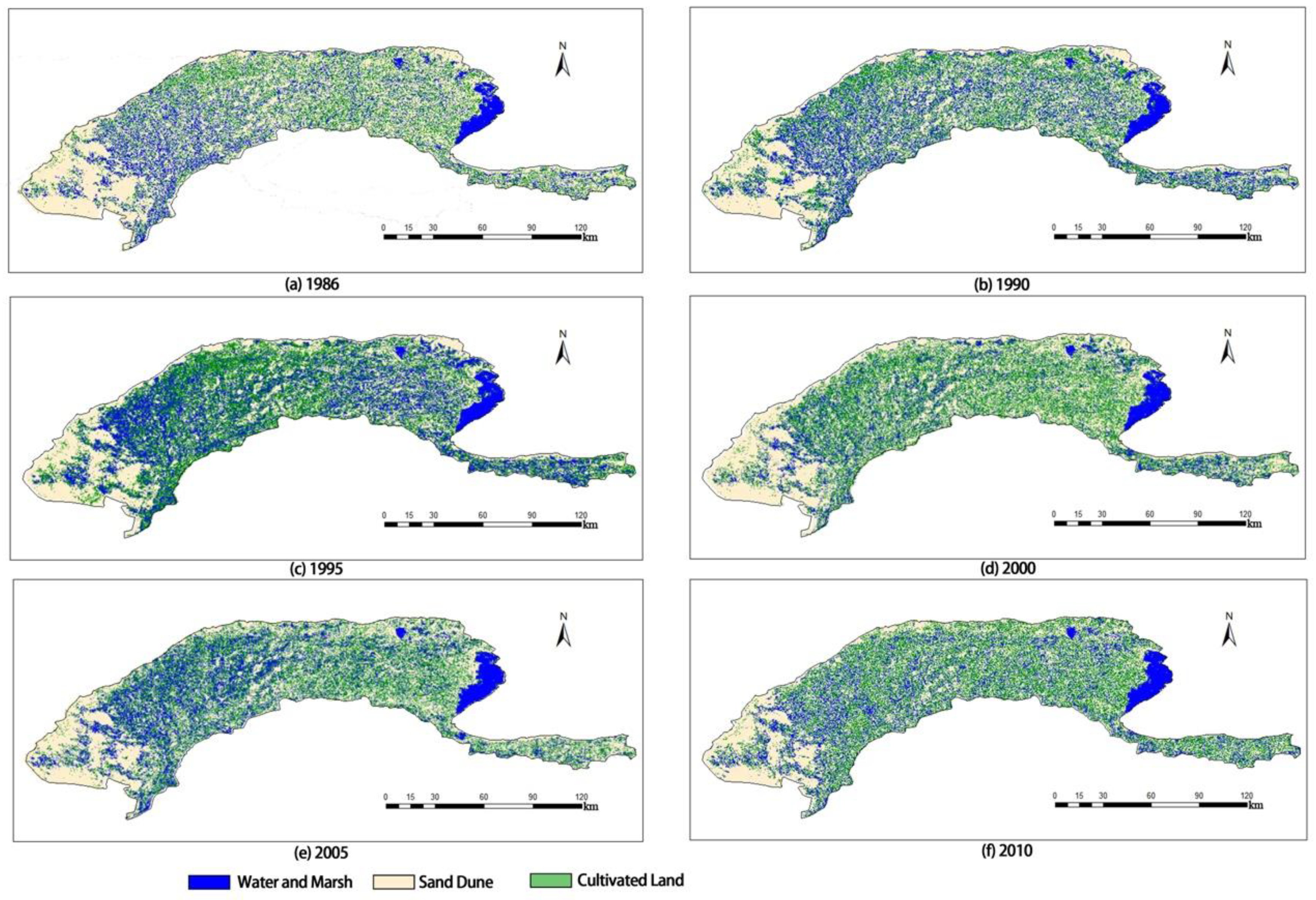
4.2.1. Detection of Cultivated Land Area

The classification maps of the total cultivated land area of HID in 1986, 1990, 1995, 2000, 2005, and 2010, respectively, are shown in Figure 9. These maps were obtained using the image segmentation method with the green pixel representing the cultivated land for agriculture. Based on the remote sensing estimation, the cultivated land area increased from 355,926 ha in 1986 to 553,923 ha in 2010, indicating approximately a onefold increase during this 24-year period. The fastest increasing stage for cultivated land was found in 1995–2000 with an increasing rate of 20,158.5 ha/year. In contrast, the sand dune (i.e. pale-yellow pixels in Figure 8) area decreased from 334,012 ha in 1986 to 233,230 ha in 2010, indicating a decrease of 30.17%. The most obvious decrease of sand dune area occurred in 2000–2005 with a decreasing area of 67,830 ha. Whereas the area of the water body and marsh (see the blue pixels in Figure 9) decreased from 231,519 ha in 1986 to 132,950 ha in 2010. Figure 10 shows the comparison of the statistical data and the cultivated land area estimated by remote sensing. It can be seen that the estimated area of the cultivated land had a similar increasing trend as the statistical data but showed smaller than the later one. This might be attributed to, first, the statistical data was slightly higher than the practical situation, and second, the Landsat data with a resolution of 30 × 30 m or 15 × 15 m might not fully capture the cultivation details.

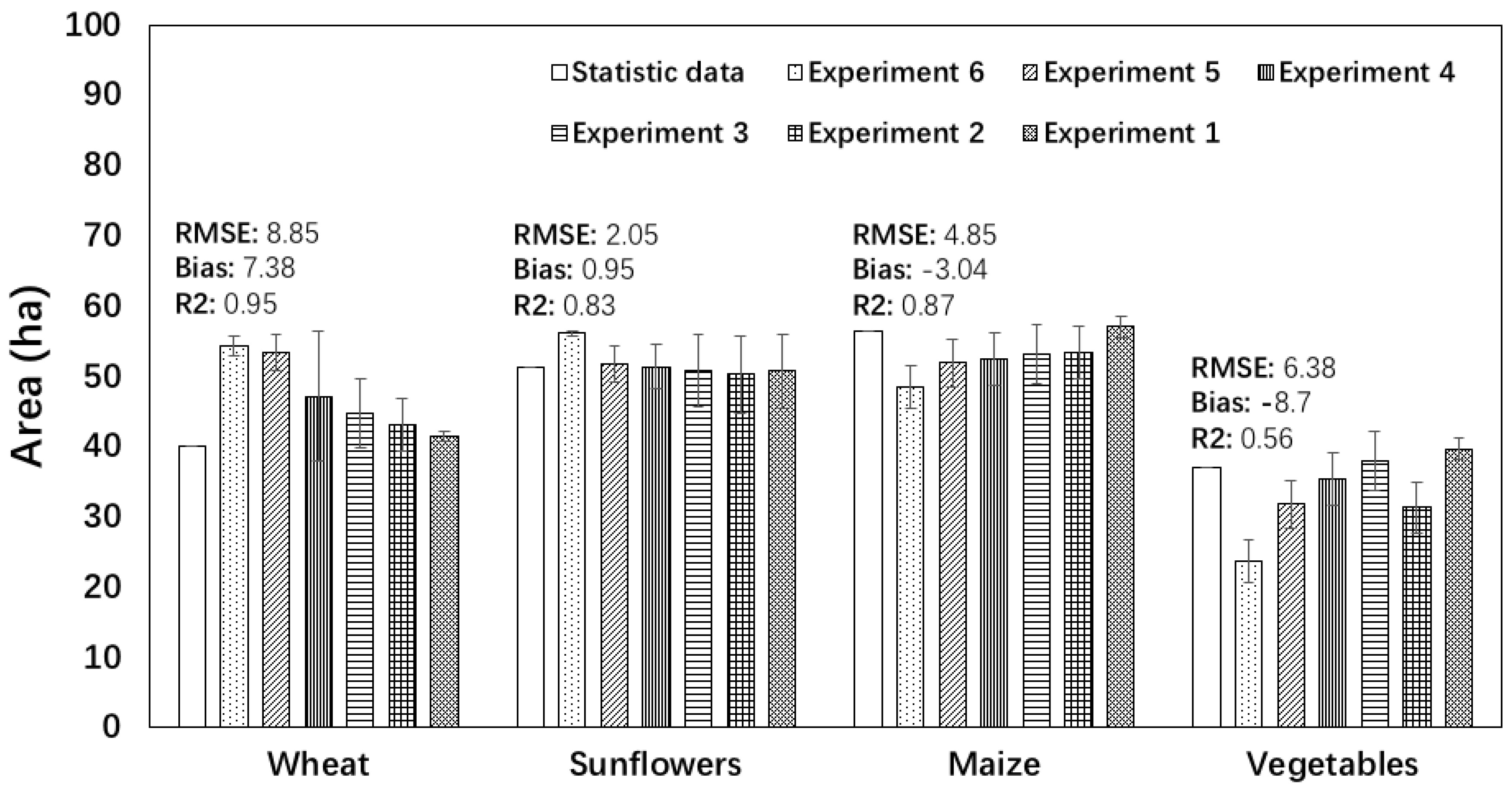
4.2.2. Classification of Planting Structure

The SS-ELM algorithm was then used to obtain the classification of agricultural planting structure in HID from 1986 to 2010, and the results are presented in Figure 11 and

Table 5. Comparison of the area estimated by remote sensing and the statistical data for maize, wheat, and sunflowers in different years.

No.	Year	Area Estimated by Remote Sensing (ha)			Statistical Area (ha)
		Maize	Wheat	Sunflowers	Maize	Wheat	Sunflowers
1	1986	36,276 (14.51%)	151,781 (60.73%)	61,836 (24.74%)	30,646	168,120	51,226
2	1990	42,272 (11.90%)	250,158 (70.47%)	62,539 (17.61%)	40,746	228,960	69,846
3	1995	52,674 (12.02%)	300,400 (68.46%)	85,025 (19.40%)	45,553	246,206	82,806
4	2000	53,328 (13.67%)	209,402 (53.70%)	127,187 (32.61%)	59,024	202,625	146,024
5	2005	89,593 (22.99%)	155,997 (40.03%)	144,051 (36.97%)	77,480	173,027	143,188
6	2010	106,322 (27.87%)	105,403 (27.63%)	169,700 (44.49%)	99,754	84,384	210,620

. As shown in Figure 11, wheat, maize, and sunflowers respectively corresponding to the color blocks of yellow, green, and purple in the resulting maps, were the three major planting crops. Of the three crops, the proportion of wheat planting area showed a significant decreasing trend. In contrast, the proportions of maize and sunflowers planting areas had a steadily increasing trend during the period of 1986–2010. Among these three crops, wheat was the crop with the largest planting area accounting for 70% of the total planting area in 1990 and became a crop with its area only about 28% of the total planting area in 2010. Meanwhile, the proportion of planting area was 12% for maize and 17% for sunflowers in 1990, and it increased to 28% for maize and 44% for sunflowers in 2010, respectively.

As shown in Table 5, during the period of 1986–2010, the total planting area of the three main crops increased from 249,893 ha in 1986 to 381,425 ha in 2010, indicating an increasing rate of 52.64%. Of these three main crops, the wheat planting area increased before 1995 with an annual increase of 16,513 ha/year, and then decreased in the following years with a decreasing rate of 12,999 ha/year. However, the planting areas of maize and sunflowers showed a continuous increase, and the values for maize and sunflowers in 2010 were 2.9 and 2.7 times as large as those in 1986, respectively. Especially, a significantly increasing trend could be identified with an increasing rate of 68% for maize from 2000 to 2005, and 49% for sunflowers from 1995 to 2000, respectively. In addition, the remote sensing estimated areas of the three crops were basically consistent with the statistical data, and the average difference between the estimated value and the statistical data was within 14%. The result indicated that the SS-ELM algorithm has good accuracy for the classification of crop planting structure in large-scale areas. The discrepancy between the estimated value and the statistical data again might be attributed to the fact that at first, the remote sensing image might not fully capture the detail cropping pattern, and second, a bias might exist between the statistical data and the practical cropping area.

The cultivation land area and the total planting area of the three main crops (wheat, maize, and sunflowers) in HID have dramatically increased from 1986 to 2010. This might be attributed to an increase in the local population, increasing food requirements. In addition, with economic development, expanding the cultivated land area and planting area is one of the major channels for local farmers to increase their income [39]. However, regional water-saving policies and the economic consideration of crop production might be two important reasons for the great changes in planting structures [40,41], causing the increase of the planting areas of maize and sunflowers and the decrease of wheat planting area during the period of 1986–2010. Especially, the comprehensive water-saving practices have been adopted in HID since 2000, which aims to reduce the diversion of water from the Yellow River [40]. As one of the major practices, planting structure adjustments by increasing high economic benefit and water-saving crops (sunflowers and maize) and reducing the crops with low economic benefit and high water consumption (wheat) has also been performed as well [41]. This then largely alleviates water shortages in HID, while effectively protecting the farmers’ income. In addition to being used to observe land-use changes in the early years, the agricultural planting structure map can be used as the basic data for hydrological modelling and other surface parameters reproduction.

Compared with the semi-supervised Laplacian extreme learning machine, the SS-ELM algorithm combined with the co-training self-label algorithm is more suitable to solve the problem of agricultural planting structure classification. The co-training algorithm trains two robust classifiers with the labeled samples in two independent subsets, and then selects the unlabeled samples with high reliability to train the other classifier separately. This method not only solves the problem of the amount and quality of manually labeled data but also makes the samples with low resolution be labeled more correctly. The image segmentation with k-means makes the classification of agricultural planting structure directly eliminate the interference of non-agricultural lands, thus reducing the amount of time needed for classification.

It should also be mentioned that the SS-ELM method performs classification iteratively. The iterative procedure is also adopted by the active learning method [42,43,44,45]. Both the active learning and the semi-supervised learning methods use the unlabeled and labeled data to improve their learning ability. The main idea of the active learning is different from that of the semi-supervised learning. The active learning method needs an external entity to annotate the request, whereas the semi-supervised learning method does not need manual intervention. The active learning method shows good performance on hyperspectral image classification based on neural network, graph, spatial prior fuzziness pool, or 3d-gabor. The limitation of this method is that it cannot establish a reasonable network, graph, fuzziness pool, or effective features for the classification of low-resolution images. The SS-ELM algorithm combines two robust classifiers, i.e., SVM and ELM, and shows excellent stability for the cases with low resolution images. Moreover, the classified results of using the SVM and ELM classifiers are even more reliable than the manually classified results. This advantage is particularly prominent in the classification of the complex agricultural planting structure.

5. Conclusions

In this paper, a semi-supervised extreme learning machine (SS-ELM) framework was improved and used for the classification of land cultivation and agricultural planting structure. The SS-ELM performs the classification by jointly using the image segmentation, the self-label algorithm and the extreme learning machine based on the remote sensing data. The classification framework was evaluated by using the experiments with datasets collected from a small-scale area, and the results with reasonable accuracy were achieved even with a small number of labeled samples. Then the SS-ELM algorithm was used for the detection of land cultivation and the classification agricultural planting structure in HID, a large-scale agricultural area in the upper reaches of the Yellow River basin. The areas of both the cultivated land and the major planting crops estimated using the SS-ELM algorithm were consistent with the statistical data.

Compared with the traditional supervised and the semi-supervised algorithms, the SS-ELM algorithm could obtain the agricultural planting results with much higher accuracy and efficiency. Especially, for the cases without sufficient identified samples for each crop category, the SS-ELM algorithm could effectively solve the problem because the framework can label a sufficient number of unlabeled target samples and use the enlarged sample set for classification. Thus, it can improve the detection and classification ability and efficiency of land cultivation and planting structure.

However, in the classification of agricultural planting structure, it always occurs that crops with small growing area, e.g., vegetables and oilseed crops in HID, cannot be identified from those crops with large growing area, e.g., wheat, maize, and sunflowers in HID. In addition, the performance of SS-ELM algorithm is sensitive to the accuracy of image recognition of planting structures. Further studies are therefore required to apply the high-resolution remote sensing images which have been developed in recent years for improving the classification accuracy of agricultural planting structure. In addition, techniques of advanced computer vision, e.g., deep learning, can also be used to improve the recognition accuracy and efficiency of land cultivation and agricultural planting structure.

References

1. Li, Y.; Zhang, H.; Xue, X.; Jiang, Y.; Shen, Q. Deep learning for remote sensing image classification: A survey. WIREs Data Min. Knowl. Discov. 2018, e1264. [Google Scholar] [CrossRef] [Green Version]
2. Rodriguez-Galiano, V.; Ghimire, B.; Rogan, J.; Chicaolmo, M.; Rigol-Sanchez, J. An assessment of the effectiveness of a random forest classifier for land-cover classification. ISPRS J. Photogramm. Remote Sens. 2012, 67, 93–104. [Google Scholar] [CrossRef]
3. Li, J.; Xi, B.; Du, Q.; Song, R.; Li, Y.; Ren, G. Deep Kernel Extreme-Learning Machine for the Spectral–Spatial Classification of Hyperspectral Imagery. Remote Sens. 2018, 10, 2036. [Google Scholar] [CrossRef] [Green Version]
4. Sandino, J.; Gonzalez, L.; Mengersen, K.; Gaston, K. UAVs and machine learning revolutionising invasive grass and vegetation surveys in remote arid lands. Sensors 2018, 18, 605. [Google Scholar] [CrossRef] [Green Version]
5. Garea, A.S.; Heras, D.B.; Argüello, F. GPU classification of remote-sensing images using kernel ELM and extended morphological profiles. Int. J. Remote Sens. 2016, 37, 5918–5935. [Google Scholar] [CrossRef]
6. Han, W.; Feng, R.; Wang, L.; Cheng, Y. A semi-supervised generative framework with deep learning features for high-resolution remote sensing image scene classification. ISPRS J. Photogramm. Remote Sens. 2018, 145, 23–43. [Google Scholar] [CrossRef]
7. Townsend, P.A.; Walsh, S.J. Remote sensing of forested wetlands: Application of multitemporal and multispectral satellite imagery to determine plant community composition and structure in southeastern USA. Plant Ecol. 2001, 157, 129–149. [Google Scholar] [CrossRef]
8. Zanotta, D.C.; Zortea, M.; Ferreira, M.P. A supervised approach for simultaneous segmentation and classification of remote sensing images. ISPRS J. Photogramm. Remote Sens. 2018, 142, 162–173. [Google Scholar] [CrossRef]
9. Kestur, R.; Angural, A.; Bashir, B.; Omkar, S.N.; Anand, G.; Meenavathi, M.B. Tree crown detection, delineation and counting in UAV remote sensed images: A neural network based spectral–spatial method. J. Indian Soc. Remote 2018, 46, 991–1004. [Google Scholar] [CrossRef]
10. Adhikary, S.K.; Dhekane, S.G. Hyperspectral image classification using semi-supervised random forest. In Proceedings of the International Conference on ISMAC in Computational Vision and Bio-Engineering, Palladam, India, 16–17 May 2018. [Google Scholar] [CrossRef]
11. Yan, D.; Chu, Y.; Li, L.; Liu, D. Hyperspectral remote sensing image classification with information discriminative extreme learning machine. Multimed. Tools Appl. 2018, 77, 5803–5818. [Google Scholar] [CrossRef]
12. Weng, Q.; Mao, Z.; Lin, J.; Liao, X. Land-use scene classification based on a CNN using a constrained extreme learning machine. Int. J. Remote Sens. 2018, 39, 6281–6299. [Google Scholar] [CrossRef]
13. Wang, L.; Hao, S.; Wang, Q.; Wang, Y. Semi-supervised classification for hyperspectral imagery based on spatial-spectral label propagation. ISPRS J. Photogramm. Remote Sens. 2014, 97, 123–137. [Google Scholar] [CrossRef]
14. Xu, Y.; Du, B.; Zhang, F.; Zhang, L. Hyperspectral image classification via a random patches network. ISPRS J. Photogramm. Remote Sens. 2018, 142, 344–357. [Google Scholar] [CrossRef]
15. Yang, C.; Li, Q.; Hu, Z.; Chen, J.; Shi, T.; Ding, K.; Wu, G. Spatiotemporal evolution of urban agglomerations in four major bay areas of US, China and Japan from 1987 to 2017: Evidence from remote sensing images. Sci. Total Environ. 2019, 671, 232–247. [Google Scholar] [CrossRef]
16. Lei, Y.X.; Chen, X.F.; Min, M.; Xie, Y.F. A semi-supervised laplacian extreme learning machine and feature fusion with cnn for industrial superheat identification. Neurocomputing 2020, 381, 186–195. [Google Scholar] [CrossRef]
17. Huang, G.; Song, S.; Gupta, J.N.D.; Wu, C. Semi-supervised and unsupervised extreme learning machines. IEEE Trans. Cybern. 2017, 44, 2405–2417. [Google Scholar] [CrossRef]
18. Zhou, W.; Qiao, S.; Yi, Y.; Han, N.; Chen, Y.; Lei, G. Automatic optic disc detection using low-rank representation based semi-supervised extreme learning machine. Int. J. Mach. Learn. Cybern. 2019, 11, 55–69. [Google Scholar] [CrossRef]
19. Krishnapuram, B.; Carin, L.; Figueiredo, M.A.T.; Hartemink, A.J. Sparse multinomial logistic regression: Fast algorithms and generalization bounds. IEEE Trans. Pattern Anal. Mach. Intell. 2005, 27, 957–968. [Google Scholar] [CrossRef] [Green Version]
20. Rosenberg, C.; Hebert, M.; Schneiderman, H. Semi-Supervised Self-Training of Object Detection Models. In Proceedings of the 7th IEEE Workshop on Application of Computer Vision, Breckenridge, CO, USA, 5–7 January 2005; pp. 29–36. [Google Scholar] [CrossRef]
21. Ando, R.K.; Zhang, T. Two-view feature generation model for semi-supervised learning. In Proceedings of the 24th International Conference on Machine Learning, Corvallis, OR, USA, 20–24 June 2007; pp. 25–32. [Google Scholar]
22. Joachims, T. Transductive Inference for Text Classification Using Support Vector Machines. In Proceedings of the 16th International Conference on Machine Learning, Bled, Slovenia, 27–30 June 1999; pp. 200–209. [Google Scholar]
23. Blum, A.; Chawla, S. Learning from Labeled and Unlabeled Data Using Graph Mincuts. In Proceedings of the 18th International Conference on Machine Learning, Williamstown, MA, USA, 28 June–1 July 2001; pp. 19–26. [Google Scholar]
24. Banerjee, B.; Buddhiraju, K.M. A novel semi-supervised land cover classification technique of remotely sensed images. J. Indian Soc. Remote Sens. 2015, 43, 719–728. [Google Scholar] [CrossRef]
25. Balabantaray, R.C.; Sarma, C.; Jha, M. Document clustering using k-means and k-medoids. Int. J. Knowl. Based Comput. Syst. 2013, 1, 1–5. [Google Scholar]
26. Hu, G.; Zhou, S.; Guan, J.; Hu, X. Towards effective document clustering: A constrained k-means based approach. Inform. Process. Manag. 2008, 44, 1397–1409. [Google Scholar] [CrossRef]
27. Wang, L. On the euclidean distance of image. IEEE Trans. Pattern Anal. 2005, 27, 1334–1339. [Google Scholar] [CrossRef] [PubMed]
28. Celebi, M.E.; Kingravi, H.A. Linear, deterministic, and order-invariant initialization methods for the k-means clustering algorithm. In Partitional Clustering Algorithms; Celebi, M., Ed.; Springer: Cham, Switzerland, 2015. [Google Scholar]
29. Celebi, M.E.; Kingravi, H.A.; Vela, P.A. A comparative study of efficient initialization methods for the k-means clustering algorithm. Expert Syst. Appl. 2013, 40, 200–210. [Google Scholar] [CrossRef] [Green Version]
30. Huang, G.B.; Zhu, Q.; Siew, C. Extreme learning machine: Theory and applications. Neurocomputing 2006, 70, 489–501. [Google Scholar] [CrossRef]
31. Yang, C.; Liu, H.; Liao, S.; Wang, S. Extreme learning machine-guided collaborative coding for remote sensing image classification. In Proceedings of the Extreme Learning Machine Conference, ELM-2015, Hangzhou, China, 15–17 December 2015; Springer International Publishing: Cham, Switzerland, 2016; Volume 1. [Google Scholar] [CrossRef]
32. Huang, G.-B.; Chen, L.; Siew, C.-K. Universal Approximation Using Incremental Constructive Feedforward Networks With Random Hidden Nodes. IEEE Trans. Neural Netw. 2006, 17, 879–892. [Google Scholar] [CrossRef] [PubMed] [Green Version]
33. Huang, G.-B.; Zhou, H.; Ding, X.; Zhang, R. Extreme Learning Machine for Regression and Multiclass Classification. IEEE Trans. Syst. Man. Cybern. 2011, 42, 513–529. [Google Scholar] [CrossRef] [Green Version]
34. Huang, G.-B.; Bai, Z.; Kasun, L.L.C.; Vong, C.M. Local Receptive Fields Based Extreme Learning Machine. IEEE Comput. Intell. Mag. 2015, 10, 18–29. [Google Scholar] [CrossRef]
35. Han, M.; Liu, B. Ensemble of extreme learning machine for remote sensing image classification. Neurocomputing 2015, 149, 65–70. [Google Scholar] [CrossRef]
36. Huang, F.; Lu, J.; Tao, J.; Li, L.; Tan, X.; Liu, P. Research on Optimization Methods of ELM Classification Algorithm for Hyperspectral Remote Sensing Images. IEEE Access 2019, 7, 108070–108089. [Google Scholar] [CrossRef]
37. Scardapane, S.; Fierimonte, R.; Di Lorenzo, P.; Panella, M.; Uncini, A. Distributed semi-supervised support vector machines. Neural Netw. 2016, 80, 43–52. [Google Scholar] [CrossRef]
38. Segal, M.R. Machine Learning Benchmarks and Random Forest Regression; Center for Bioinformatics & Molecular Biostatistics, UC San Francisco: San Francisco, CA, USA, 2004; Available online: http://escholarship.org/uc/item/35x3v9t4 (accessed on 14 April 2003).
39. Zhu, Z. Analysis on Water-Saving Measures and Estimation on Water-Saving Potential of Agricultural Irrigation in Hetao Irrigation District of Inner Mongolia. Ph.D. Thesis, Yangzhou University, Yangzhou, China, June 2017. [Google Scholar]
40. Tong, W. Study on Salt Tolerance of Crops and Cropping System Optimization in Hetao Irrigation District. Ph.D. Thesis, China Agricultural University, Beijing, China, June 2014. [Google Scholar]
41. Fu, W.; Zhai, J.; Zhao, Y.; He, G.; Zhang, Y. Effects of the Planting Structure Adjustment on Water Budget of Field System in Hetao Irrigation Area. J. Irrig. Drain. 2017, 36, 1–8. [Google Scholar] [CrossRef]
42. Ahmad, M.; Khan, A.; Khan, A.M.; Mazzara, M.; Nibouche, O. Spatial prior fuzziness pool-based interactive classification of hyperspectral images. Remote Sens. 2019, 1, 1136. [Google Scholar] [CrossRef] [Green Version]
43. Jie, H.; Zhi, H.; Jun, L.; Lin, H.; Yiwen, W. 3d-gabor inspired multiview active learning for spectral-spatial hyperspectral image classification. Remote Sens. 2018, 10, 1070. [Google Scholar] [CrossRef] [Green Version]
44. Li, J. Active learning for hyperspectral image classification with a stacked autoencoders based neural network. In Proceedings of the 2016 IEEE International Conference on Image Processing (ICIP), Phoenix, AZ, USA, 25–28 September 2016. [Google Scholar]
45. Ni, D.; Ma, H. Active learning for hyperspectral image classification using sparse code histogram and graph-based spatial refinement. Int. J. Remote Sens. 2017, 38, 923–948. [Google Scholar] [CrossRef]
Figure 1. The Yellow River basin and location of the study area, Hetao irrigation district (HID).
Remotesensing 12 03708 g001
Figure 2. Examples of land use pattern.
Remotesensing 12 03708 g002
Figure 3. Flowchart of the semi-supervised extreme learning machine (SS-ELM) framework.
Remotesensing 12 03708 g003
Figure 4. Flowchart of the ELM algorithm.
Remotesensing 12 03708 g004
Figure 5. Flowchart of self-label algorithm.
Remotesensing 12 03708 g005
Figure 6. Comparison of the classification maps of experiment 4 using different algorithms, (a) original image, (b) handcrafted classified image, (c) RF classification results, (d) SVM classification results, (e) ELM classification results, (f) S-SVM classification results, and (g) SS-ELM classification results.
Remotesensing 12 03708 g006
Figure 7. The classification maps of SS-ELM experiments, (a) experiment 1, (b) experiment 2, (c) experiment 3, (d) experiment 4, (e) experiment 5, (f) experiment 6.
Remotesensing 12 03708 g007
Figure 8. Comparison of the statistical data and the remote sensing estimated areas for wheat, sunflowers, maize, and vegetables.
Remotesensing 12 03708 g008
Figure 9. Image segmentation results of the Hetao Irrigation District in 1986–2010.
Remotesensing 12 03708 g009
Figure 10. Estimated area of different land use (a) and comparison of the statistical data and the cultivated land area estimated by remote sensing (b).
Remotesensing 12 03708 g010
Figure 11. Planting structure classification results of the Hetao Irrigation District in 1986–2010.
Remotesensing 12 03708 g011