Abstract
With the rapid process of urbanization, anthropogenic heat generated by human activities has become an important factor that drives the changes in urban climate and regional environmental quality. The nighttime light (NTL) data can aptly reflect the spatial distribution of social-economic activities and energy consumption, and quantitatively estimate the anthropogenic heat flux (AHF) distribution. However, the commonly used DMSP/OLS and Suomi-NPP/VIIRS NTL data are restricted by their coarse spatial resolution and, therefore, cannot exhibit the spatial details of AHF at city scale. The 130 m high-resolution NTL data obtained by Luojia 1-01 satellite launched in June 2018 shows a promise to solve this problem. In this paper, the gridded AHF spatial estimation is achieved with a resolution of 130 m using Luojia 1-01 NTL data based on three indexes, NTLnor (Normalized Nighttime Light Data), HSI (Human Settlement Index), and VANUI (Vegetation Adjusted NTL Urban Index). We chose Jiangsu, a fast-developing province in China, as an example to determine the best AHF estimation model among the three indexes. The AHF of 96 county-level cities of the province was first calculated using energy-consumption statistics data and then correlated with the corresponding data of three indexes. The results show that based on a 5-fold cross-validation approach, the VANUI power estimation model achieves the highest R2 of 0.8444 along with the smallest RMSE of 4.8277 W·m−2 and therefore has the highest accuracy among the three indexes. According to the VANUI power estimation model, the annual mean AHF of Jiangsu in 2018 was 2.91 W·m−2. Of the 96 cities, Suzhou has the highest annual mean AHF of 7.41 W·m−2, followed by Wuxi, Nanjing, Changzhou and Zhenjiang, with the annual mean of 3.80–5.97 W·m−2, while the figures of Suqian, Yancheng, Lianyungang, and Huaian, the cities in northern Jiangsu, are relatively low, ranging from 1.41 to 1.59 W·m−2. This study has shown that the AHF estimation model developed by Luojia 1-01 NTL data can achieve higher accuracy at city-scale and discriminate the spatial detail of AHF effectively.
1. Introduction
With the rapid development of urbanization, urban built-up areas have expanded dramatically. A number of natural landscapes have been replaced with various artificial surface, which causes sensible heat increases and latent heat decreases, resulting in an urban heat island (UHI) [1,2]. At the same time, the number of urban populations has continued to surge. According to the statistics from the United Nations Population Division, the proportion of world’s urban population has surged from 30% in 1950 to 55.3% in 2018, and which is expected reach 68% by 2050 [3]. Intensive human activities consume a lot of energy resources, and eventually release not only greenhouse gases, aerosols, and other harmful substances into the atmosphere, but also large amounts of anthropogenic heat [4]. A large amount of anthropogenic heat emissions affects the energy exchange between the land surface and atmosphere within the cities and aggravates the temperature rise in urban and surrounding areas. Much research in recent years has shown that anthropogenic heat is one of the key contributing factors to forming UHI and has a significant impact on local climate [5,6]. Therefore, it is very important to accurately quantify the anthropogenic heat for monitoring the UHI effect and improving the urban environments [7].
Anthropogenic heat flux (AHF) refers to the amount of anthropogenic heat emissions generated per unit time and unit area [8]. Earlier, Torrance and Shun [9] paid attention to urban anthropogenic heat and its impacts on urban climate. Subsequently, many researchers also launched studies on anthropogenic heat to estimate the AHF in cities and regions [10,11]. Wang et al. [12] estimated the annual mean AHF of China in 2016 and found that at the provincial level, the AHF of Shanghai is the highest which reaches 12.53 W·m−2, followed by Tianjin, Beijing, and Guangdong, the AHF values are 6.91 W·m−2, 5.84 W·m−2, and 4.53 W·m−2, respectively. According to the model predicted by Flanner [13], the annual mean AHF over continental United States, western Europe and China, 2005 AHF values are 0.39 W·m−2, 0.68 W·m−2, and 0.22 W·m−2, respectively. Moreover, in 2040, these regional annual mean AHF will increase to 0.59 W·m−2, 0.89 W·m−2, and 0.76 W·m−2. Moreover, the global distributions of annual mean AHF for 2005 and 2040 are 0.028 W·m−2 and 0.059 W·m−2. In addition, he pointed out that the increase of global average annual AHF will aggravate the rise of global average temperature, and cause aerosol and other atmospheric pollutants in planetary boundary layer release into the areas with high AHF.
Nighttime light (NTL) data has a unique capability to detect low levels of visible and near-infrared (VNIR) radiance emissions from cities and towns at night [14]. The brightness of NTL can reflect the spatial distribution of social economic activities and energy consumptions [15,16]. Moreover, many researchers have found that there is a significant correlation between the brightness of NTL and AHF [12,17,18], which could be used for AHF spatial gridding estimation. Wang et al. [12] found that the normalized NPP/VIIRS NTL data is highly correlated with AHF, where the fitting R2 is 0.95. Chen et al. [18] established the quantitative relationship between NTL and AHF to estimate the anthropogenic heat release distribution in China from 1992 to 2009. There is a strong negative correlation between vegetation coverage and impervious surface, that is, the areas with higher density impervious surface have lower vegetation coverage. This conclusion has been proven by many studies [19,20]. Therefore, some researchers combined vegetation indexes with NTL data to reduce saturation and increase variation in nighttime luminosity, thereby improving the fitting relationships between NTL data and AHF. Lu et al. [21] combined DMSP/OLS NTL data with MODIS NDVI vegetation products to construct the Human Settlement Index (HSI). Chen and Hu [22] found a strong correlation between the annual mean AHF and mean HSI (R2 = 0.98). Ma et al. [23] obtained the gridded AHF estimation result in Zhejiang Province, China, based on HSI. Moreover, Zhang et al. [24] used the vegetation index to reduce saturation of the NTL data values in core urban areas and proposed the Vegetation Adjusted NTL Urban Index (VANUI).
At present, the two generations of NTL sensors, DMSP/OLS and Suomi-NPP/VIIRS, are the most widely used NTL data with coarse spatial resolutions 1000 m and 500 m, respectively [25]. In June 2018, Luojia 1-01 scientific experimental satellite was successfully launched [26]. Luojia 1-01 is China’s advanced NTL remote sensing satellite with 130 m spatial resolution and 14-bit radiometric resolution [25,27], which provides a critical basis data for refining the estimation of gridded AHF. Currently, there are few studies on this subject. Therefore, this study aims to construct the AHF spatial estimation models based on Luojia 1-01 NTL data, realize the AHF gridding estimation and mapping with a high resolution of 130 m in Jiangsu Province, China, in the year 2018. First, the AHF of 96 county-level cities of Jiangsu are calculated using energy-consumption statistics data. Next, the relationships between the 96 county-level cities’ AHF and NTL related indexes, NTLnor, HIS, and VANUI, are established, thereby the AHF spatial estimation models of Jiangsu are constructed. Then, the performance and accuracy of different AHF estimation models are analyzed and compared, and the best model is determined based on a 5-fold cross-validation approach. Finally, the AHF mapping with a high resolution of 130 m is realized and the spatial distribution characteristics of AHF in urban areas are analyzed based on the AHF estimation result.
2. Methods
2.1. Study Area
The study area is Jiangsu Province, located in China’s southeastern coastal region (30°45′N–35°20′N, 116°18′E–121°57′E). Jiangsu belongs to a subtropical and warm temperature climate transition zone with the average annual temperature around 13–16℃, the average annual rainfall between 150–400 mm. The regional gross domestic product (GDP) of Jiangsu increased from 4196.2 billion yuan in 2010 to 9259.5 billion yuan in 2018, with a growth rate of 121%, and the GDP per capita increased from 53,525 yuan to 115,168 yuan, ranking first among all the provinces in China. The total population increased from 78.7 million people to 80.5 million people. Moreover, the energy consumption also increased significantly, from 257.7 million tons of standard coal in 2010 to 314.3 million tons of standard coal in 2018 [28]. Jiangsu Province is divided into 13 prefecture-level cities (Nanjing, Wuxi, Xuzhou, Changzhou, Suzhou, Nantong, Liangyungang, Huaian, Yancheng, Yangzhou, Zhenjiang, Taizhou, and Suqian) and 96 county-level cities. The study area covers around 100,831 km2, some small coastal islands and reefs are not included in this study (Figure 1).
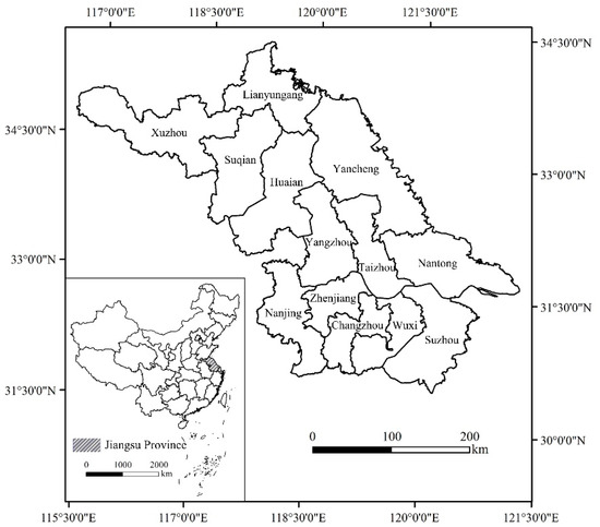
Figure 1.
Location map of Jiangsu Province.
Figure 2 is the land cover map of Jiangsu, the dataset of 30-m Finer Resolution Observation and Monitoring-Global Land Cover (FROM-GLC30) by Gong et al. [29]. It can be seen from Figure 2 that the northern and central of Jiangsu are predominated by cropland, and the south has a large area of continuous impervious surface. Statistics show that the area is dominated by cropland, making up 66.11% of the area, followed by impervious surface (16.81%), water (11.72%), and forest (4.12%).
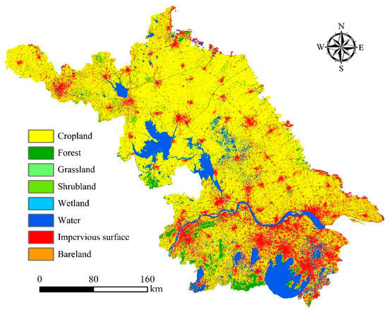
Figure 2.
Land cover map of Jiangsu.
The development difference between north and south regions in Jiangsu is obvious. The cities in the south have faster economic growth and larger population inflow than those in the north. Therefore, this study can reveal the regional unbalanced development and the spatial distribution characteristics of AHF in Jiangsu, which is of great significance for the study of anthropogenic heat emissions.
2.2. Satellite Data
The NTL data used in this study is Luojia 1-01. We acquired all the GEC system geometry corrected NTL products covering Jiangsu in 2018, downloaded from the High-Resolution Earth Observation System of the Hubei Data and Application Center (http://www.hbeos.org.cn).
Since some AHF algorithms used in this article need the help of vegetation index, we further selected the Landsat 8 images in 2018. The product level of Landsat 8 images is Level 1T, downloaded from the United States Geological Survey (USGS) (https://earthexplorer.usgs.gov/). The acquisition time of Landsat 8 images had to be selected in summer from July to August as far as possible, because the images of the optimum growth of vegetation throughout the year in 2018 needed to be utilized in this study. However, there are many cloudy and rainy days in summer of subtropical area like Jiangsu, so a large number of Landsat 8 images are missing. The images from June to October were used as supplements, because Jiangsu is dominated by evergreen vegetation, and the growth trends of vegetation from June to October are relatively similar.
2.3. Remote Sensing Data Processing
Although the system geometry was corrected before being downloaded, Luojia 1-01 images still had slight geo-referencing errors by about 150–400 m, when referring to the Landsat 8 images. In order to ensure the accuracy of overlay analysis, a map-to-map geometric correction was performed. Taking Landsat 8 as the reference image, Luojia 1-01 was registered with Landsat 8.
Jiangsu is covered by multiple scene images of Luojia 1-01 images on different acquisition dates. In order to ensure the continuity of the spatial pixels, and eliminate the lighting noise existing in the NTL data, the overlapping areas were averaged for the brightness of light, and if the pixels in an image were 0, then this position was represented by 0 [30]. Then, the DN value image of NTL data of Jiangsu was obtained by mosaicking and clipping the processed images.
We detected a few outliers in the Luojia 1-01 NTL mosaicking image. The outliers are probably caused by the stable lights from fires of oils or gas wells located in those areas [31]. In order to correct the outliers, the processing procedure proposed by Shi et al. [31] was performed. Since Nanjing, Wuxi, and Suzhou are the three most developed cities in Jiangsu, the pixel values of the other areas should not exceed those cities theoretically. According to statistics, the highest DN value in Nanjing, Wuxi, and Suzhou is 793,457, which was used as a threshold to correct the outliers. Each pixel whose DN value was larger than 793,457 in NTL data was assigned as a new value. The new value was the maximal DN value within the pixel’s immediate eight neighbors.
The images of Landsat 8 OLI were radiometrically calibrated using the equations from the Landsat 8 Data Users Handbook [32]. This converted the DN of the raw images to at-satellite reflectance.
The Luojia 1-01 NTL and Landsat 8 images were stitched and projected to the Albers Equal Area Conic Projection, respectively. We resampled the spatial resolution of Luojia 1-01 to 30 m, consistent with Landsat 8 (Figure 3).
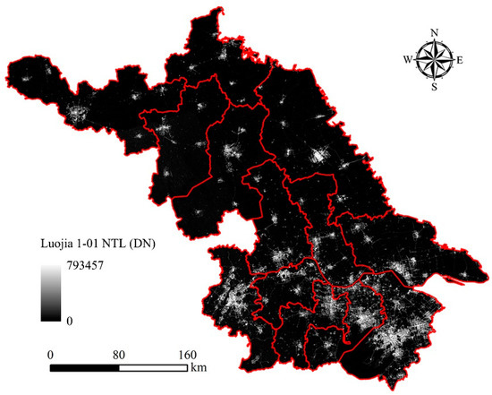
Figure 3.
Luojia 1-01 nighttime light (NTL) image of Jiangsu in 2018.
2.4. Calculation of the AHF Spatial Estimation Indexes
In this study, Normalized nighttime light data (NTLnor) [12], Human Settlement Index (HSI) [21], and Vegetation Adjusted NTL Urban Index (VANUI) [24] were employed for AHF spatial gridding estimation. In previous studies, these three indexes were calculated based on DMSP/OLS and Suomi-NPP/VIIRS NTL data. HSI and VANUI also need to integrate the brightness of NTL with MODIS vegetation index products. However, at present, there is little literature on construction of AHF estimation index based on Luojia 1-01 NTL data. Therefore, this paper attempted to transplant the three indexes to Luojia 1-01 data and combined with the Normalized Difference Vegetation Index (NDVI) [33] from Landsat 8 images for AHF estimation. The equations of NTLnor, VANUI and HSI were expressed as:
where NTLmax and NTLmin are the maximum and minimum values in NTL image, respectively; NDVImax is the maximum value in the multitemporal composite NDVI data in 2018 [21]. The NDVImax is expressed as:
where NDVI1, NDVI2, …, NDVIn are the multitemporal NDVI images from Landsat 8 in 2018.
Through visual interpretation of Google Earth satellite imagery, the pure vegetation pixels were extracted from NDVImax, with a threshold of 0.70. Each pixel whose value is larger than or equal to 0.70 in NDVImax was simply defined as pure vegetation. Furthermore, the pixels with the brightness of NTL greater than 0 were extracted from the pure vegetation. The NTLmin was obtained by counting the average brightness value of these pixels in the NTL image [34,35,36].
2.5. Estimation of the AHF of Administrative Unit Based on Statistics Data
The energy-consumption inventory approach was employed to calculate the AHF of the cities in Jiangsu based on the socio-economic data and various types of energy-consumption data from the statistical yearbook [28]. After comprehensive analysis of the statistical indicators in Jiangsu Province statistical yearbook, the four parts of anthropogenic heat emissions sources, industry, transportation, buildings (including both commercial and residential buildings), and human metabolism were considered [8,12,22,23,37,38,39,40]. The total AHF is the sum of the four parts. The equation is expressed as:
where QS is the total AHF (W·m−2); QI is the industry heat flux (W·m−2); QV is the transportation heat flux (W·m−2); QB is the buildings heat flux (W·m−2); and QM is the human metabolism heat flux (W·m−2).
The industry heat is mainly derived from various types of energy consumption, such as coal, oil, gas, electricity, etc. [12]. In addition, the actual energy consumption is converted into the standard coal. The total industry consumption of Jiangsu is calculated, then the consumption of each city is allotted based on the ratio of the secondary industry. This equation is expressed as:
where EI is the energy consumption of per ton of standard coal (tce); C is the standard coal heat, which is 29,306 kJ·kg−1 according to the national energy conversion standard; A is the study area (km2); and T is 1 year.
The transportation heat is the fuel waste heat discharged from vehicle energy consumption. The equation is expressed as:
where V is the sum of civil automobiles; D is the annual average driving distance per vehicle (km), which is assumed average 2.5 × 10⁴ km per year; E is the combustion efficiency (L·km−1), which is 12.7 L per 100 km; ρ is combustion density (kg·L−1); NHC is the net heat combustion (kJ·g−1), which is 45 kJ·g−1 [22]; A and T are the same as in Equation (6).
The buildings heat is the energy consumption from wholesale and retail trade, accommodation, catering industry, and living consumption, including commercial and residential buildings. The commercial buildings heat and residential buildings heat were allotted based on the ratio of the tertiary industry and the population in each city, respectively. The equation is expressed as:
where EBC and EBR are the commercial buildings energy consumption (tce) and residential buildings energy consumption (tce), respectively; C, A, and T are the same as in Equation (6).
The energy consumption from human metabolism is divided into two states, active (7:00~23:00) and sleeping (23:00~7:00), respectively, according to the previous studies [37,41]. The equation is expressed as:
where s1, s2 are the metabolic rate of active state (171 W per person) and sleeping state (70 W per person), respectively; t1, t2 are the hours of active time and sleeping time, respectively; P is the population; A and T are the same as in Equation (6).
2.6. Construction and Verification of the AHF Spatial Estimation Models
As was already mentioned, there is a significant correlation between brightness of NTL and AHF [17], which could be used for constructing the AHF spatial estimation model by employing the three indexes, NTLnor, HSI and VANUI). According to Equations (5)–(9), the annual mean AHF based on statistics data (AHFsta) of 96 county-level cities in Jiangsu Province can be calculated. Taking AHFsta as the dependent variable (y), and the indexes as independent variable (x), and then regression analysis was carried out to establish the gridded AHF spatial estimation models. By comparing the fitting degree (R2) of regression models based on the different indexes, the AHF estimation models with higher R2 were preliminary selected. Furthermore, we used a 5-fold cross-validation approach to evaluate the results of AHF estimation models. The 5-fold cross-validation approach can be described as follows: the dataset was split randomly into 5 subsets, 1 of which was selected as the validation subset and the remaining 4 subsets were used as the training subset. Finally, the root mean square error (RMSE) and R2 between the estimated and statistics values were employed to assess the model’s performance [42].
3. Results
3.1. Determination and Verification of the Best AHF Spatial Estimation Models
In order to realize the gridded AHF mapping and take full advantages of the high spatial resolution of Luojia 1-01 NTL data, the regression analysis of three indexes (x) and AHFsta (y) were carried out by using linear, quadratic polynomial, exponential, logarithmic, and power functions, respectively. The results of AHF spatial estimation models based on different indexes and functions are shown in Table 1. It can be seen that all the correlations are statistically significant (p < 0.005). Overall, The R2 of NTLnor and VANUI are higher than that of HSI. In term of functions, the power function has the highest R2 in the three indexes. Among them, the R2 of power function based on NTLnor and VANUI are greater than 0.83, which are much higher than 0.26 of HSI.

Table 1.
The anthropogenic heat flux (AHF) spatial estimation models based on different indexes.
Although the R2 of VANUI power function model is 0.8444, which is slightly higher than 0.8370 of NTLnor, the difference between VANUI and NTLnor is not obvious. Figure 4 gives the 5-fold cross-validation results of AHF power function estimation models based on three indexes. It shows that among the three indexes, the strongest correlations between AHFsta and AHF estimation values obtained based on VANUI model of Jiangsu’s 96 county-level cities, which yielded an R2 of 0.8228 and RMSE of 4.8277 W·m−2. Followed by the NTLnor model, which achieved a slightly low degree of agreement, with R2 of 0.8119 and RMSE of 4.9782 W·m−2. Meanwhile, the HSI model had an extremely low agreement, with the R2 value being only 0.6274, and the RMSE was as high as 7.4805 W·m−2. These results suggest that Luojia 1-01 NTL data can aptly estimate the AHF with the use of a proper index, such as VANUI or NTLnor. In this study, the estimation accuracy of VANUI is higher than that of NTLnor, so the VANUI power function model is selected as the best AHF spatial estimation model of Jiangsu in 2018.
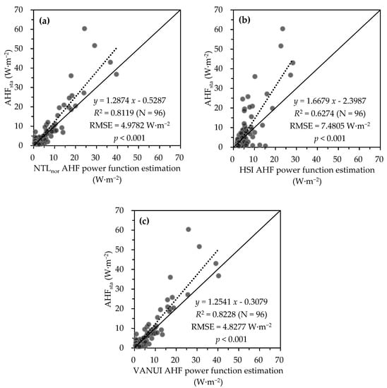
Figure 4.
Validation of AHF power function estimation models. (a) NTLnor, (b) HSI, (c) VANUI.
3.2. Analysis the Gridded AHF Mapping Results
According to the best AHF spatial estimation model of VANUI power function (y = 696.2097 x0.9304), the gridded AHF mapping of Jiangsu in 2018 with a spatial resolution of 130 m (Figure 5a) and the distribution of annual mean AHF values in each county (Figure 5b) were completed. It can be seen that the distribution of AHF in Jiangsu shows a significant difference between the north and south. In northern Jiangsu, such as Liangyungang, Huaian, Xuzhou, Yancheng, and Suqian, the AHF values are relatively low. That is because there are large areas of continuous cropland and many scattered urban built-up areas (Figure 2). Meanwhile, the AHF of cities in central Jiangsu, such as Yangzhou, Taizhou, and Nantong, have slightly higher AHF than the north. In contrast, in the south of Jiangsu, the scope of impervious surface in urban built-up areas has expanded dramatically and connected with each other (Figure 2), forming the high-value AHF areas in urban regions.
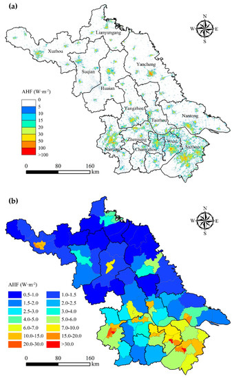
Figure 5.
The AHF estimation results of Jiangsu in 2018. (a) Gridded AHF result image, (b) County-level AHF map.
According to the statistics in Figure 5a, the annual mean AHF of Jiangsu in 2018 is 2.91 W·m−2. Among the 13 prefecture-level cities, Suzhou contributes the highest AHF, which reaches 7.41 W·m−2, followed by Wuxi, Nanjing, Changzhou, and Zhenjiang, with AHF range of 3.80–5.97 W·m−2, while the figures of Suqian, Yancheng, Lianyungang, and Huaian, the cities in northern Jiangsu, are relatively low, ranging from 1.41 to 1.59 W·m−2, only half of the whole province (Figure 6).
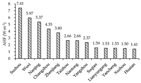
Figure 6.
The AHF estimation result of each city in Jiangsu in 2018.
Statistics of the contribution rates of AHF grades are shown in Table 2. In Jiangsu, the contribution rate of the AHF grade of 0–5 W·m−2 is the highest, reaching 87.21%. These areas with low-value AHF are mainly croplands and water, as well as a few forests. And the contribution rate of AHF >5 W·m−2 is about 12.79%. Comparing the result between AHF (Figure 5a) and land cover (Figure 2), it can be seen that the spatial distribution of AHF >5 W·m−2 is consistent with an impervious surface. It indicates that the areas with frequent human activities can be well represented by the results of AHF.
Table 2.
AHF contribution rates of different grades in Jiangsu.
3.3. Validation of AHF Estimation Results
It is difficult to validate AHF estimation results according to field measured data because the sensible or latent heat caused by human activities or background conditions cannot be completely distinguished [8,22,43]. Therefore, the results are usually verified by comparing them with previous similar studies [44,45]. Due to the inconsistency in the data sources, modeling methods, and research scales, there is often no absolute comparability between the study results, but it can be used as reference data to verify the rationality of research results as a whole [12]. Xie et al. [46], Chen et al. [18], and Wang et al. [12] employed an energy-consumption inventory approach based on statistics data to estimate the spatial distribution of AHF in China. Part of the estimation results of AHF in Jiangsu of the three existing studies are compared with those obtained in this study. The detailed comparison is shown in Table 3. The AHF estimation result in this study is basically consistent with the three existing studies results, especially in the order of magnitude.
Table 3.
The comparison of Jiangsu’s annual mean AHF estimation results in this study with the existing AHF results.
For Suzhou, Wuxi, and Nanjing, the three cities that have the highest AHF estimation values in Jiangsu, as examples (Figure 7), the spatial rationality of AHF result can be verified by comparing the distribution of AHF in the urban spaces with the different characteristics of land use and land cover types. The figure also illustrates the differences in the spatial details of AHF achieved by Luojia 1-01 and Suomi-NPP/VIIRS, respectively.
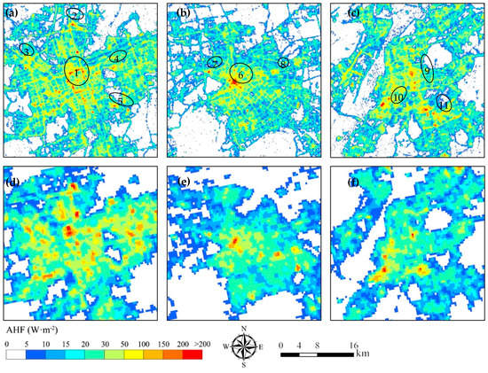
Figure 7.
AHF estimation images of Suzhou, Wuxi and Nanjing. (a–c) Luojia 1-01, (d–f) Suomi-NPP/VIIRS. 1: Suzhou ancient town, 2: Suzhou railway station and its surrounding commercial area, 3: Suzhou New District railway station, 4: Industrial district, 5: New residential and commercial high-rise real estate, 6: Wuxi city center, 7: Wuxi Baile Square city complex, 8: Wuxi Huiju city complex, 9: Nanjing Xinjiekou city center, 10: Large public buildings, 11: Nanjing South railway station.
It can be seen from Figure 7 that the gridded AHF estimation results with high resolution of 130 m based on Luojia 1-01 NTL data can effectively reveal the detailed spatial distribution of AHF inside the cities. The sharp and clear urban anthropogenic heat emissions networks are formed by the dense and orderly urban road systems. According to the different traffic flow and busy degree of the main roads, the AHF values of them vary slightly. The AHF values of urban roads are generally between 30 and 100 W·m−2. AHF can also reach more than 100 W·m−2 at some road intersections. In addition to the network distribution, AHF also forms the massive agglomeration in some prosperous areas of the city center. The high-value AHF areas are mainly distributed in urban commercial areas and old towns, such as the commercial street around the Suzhou ancient town, Wuxi city center, Baile Square and Huiju city complex, and Nanjing Xinjiekou city center. In addition, the large municipal public facilities areas, such as railway stations, the grand theatre, the international conference and exhibition center, and the Olympic center also have high AHF. The results of this study show that the AHF in these high-value areas are mostly concentrated in the range of 50–150 W·m−2, and in some extra high-value areas can exceed 200 W·m−2. Furthermore, there are some median-value areas of AHF are between 15 and 50 W·m−2; those are mainly distributed in the urban residential districts. Meanwhile, the AHF of some villages and suburban residential areas is lower, with AHF ranging of 5–15 W·m−2 (Table 4).
Table 4.
The mean AHF of the different land use types.
The above comparative analysis shows that the gridded AHF estimation results in this study have a good presentation of AHF spatial details insider the city. Furthermore, the AHF results align with the different characteristics of urban land use and land cover types in spatial distribution. To summarize, the AHF estimation in this study obtained good AHF estimation results.
4. Discussion
The AHF estimation index and its model are the key factors of AHF spatial estimation. In this study, the indexes of NTLnor, HSI, and VANUI were employed to estimate the AHF. We found that there are the significant correlations between NTLnor, VANUI. and AHFsta, especially in the power fitting equation, with R2 about 0.8. However, the AHF estimation model based on HSI, the R2 is as low as 0.26. Examining the result of HSI (Figure 8a), an unreasonable phenomenon could be found, that is, the value of water in HSI is much higher than other land covers, which directly leads to the lower fitting relationship between HSI and AHFsta. Analyzing the calculation formula of HSI in Equation (2), we found that in the extreme case, the NTL intensity of water areas should be close to 0, and the vegetation index (NDVI) with the range from −1 to 1, may be close to the minimum value, theoretically. Therefore, in this extreme situation, the HSI value in the water areas may present very high. Zhang et al. [24] also pointed out the drawbacks to the HSI. Since the relationship between NTL and NDVI follows a power law, when NTL has a maximum value, HSI will increase exponentially as NDVI approaches 0.
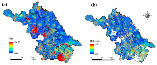
Figure 8.
The results of Human Settlement Index (HSI) (a) and HSI-water (b).
As such, when the water was removed from HSI (HSI-water) (Figure 8b), the fitting degree between HSI-water and AHFsta was greatly improved as expected (Table 5). The R2 is from 0.2641 of HSI to 0.7177 of HSI-water based on power function. The 5-fold cross-validation result of HSI-water AHF estimation model in Figure 9 illustrates that compared with HSI (R2 is 0.8887 and RMSE is 6.8358 W·m−2), HSI-water based on power function has a significant improvement in correlations (R2 is 0.8887) and accuracy (RMSE is 6.8358 W·m−2) between AHF estimation values and AHFsta values of 96 county-level cities in Jiangsu. However, if compared with VANUI (RMSE is 4.8277 W·m−2) or NTLnor (RMSE is 4.9782 W·m−2), there is still a certain accuracy gap in the result of HSI-water. Wang et al. [12] also found the same conclusion in the comparative study of these three indexes and pointed out that result of HSI have poor performance on the regional characteristics of AHF estimation.
Table 5.
The AHF spatial estimation models based on HSI-water.
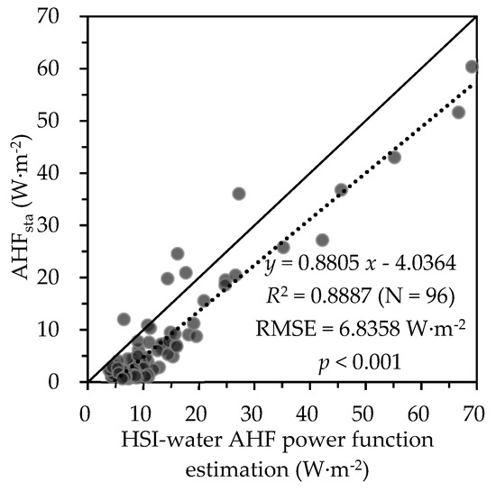
Figure 9.
Validation of AHF power function estimation models based on HSI-water.
Over the past 20 years, DMSP/OLS and Suomi-NPP/VIIRS NTL data have been proven to be useful proxy measures for monitoring and analyzing human activities [27,47,48]. The coarse spatial resolution of these NTL data often means that the studies can only be done at large scales but will be restricted at city scales.
As can be seen from the results of AHF and the comparison between Luojia 1-01 and Suomi-NPP/VIIRS in the detailed images (Figure 7) and their profiles of NTL data (Figure 10), Luojia 1-01 NTL images shows great advantages in capturing finer spatial details within urban areas. First, the main roads in urban areas can be presented more clearly by Luojia 1-01, while they are difficult to be reflected in Suomi-NPP/VIIRS. Moreover, the overall trends of the two NTL data profiles are basically similar, but the fluctuations in Luojia 1-01 are more frequently than those in Suomi-NPP/VIIRS. Moreover, the variation ranges of the peaks and valleys of Luojia 1-01 are larger than Suomi-NPP/VIIRS. These differences indicate that Luojia 1-01 NTL data contains more spatial information and has more capacities to reduce the saturation of NTL in urban areas.
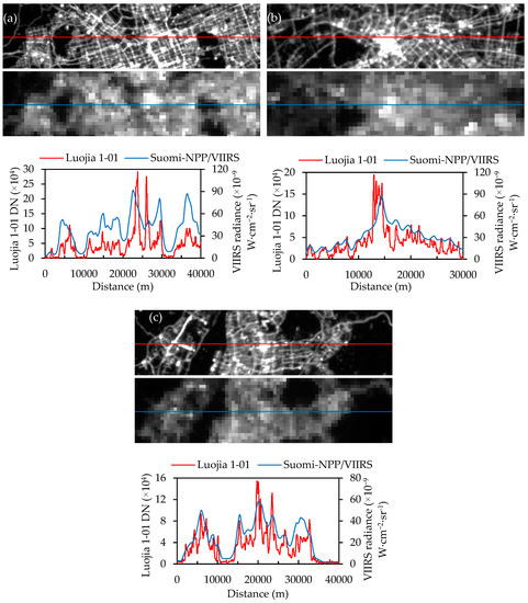
Figure 10.
The detailed images and its profiles of Luojia 1-01 and Suomi-NPP/VIIRS NTL data. (a) Suzhou, (b) Wuxi, (c) Nanjing.
5. Conclusions
In this article, using the new generation NTL data of Luojia 1-01 with finer spatial resolution, supplemented by Landsat 8 vegetation index data, the AHF spatial estimation models were constructed, and the gridded AHF mapping with high spatial resolution of 130 m in Jiangsu Province in 2018 was achieved. The conclusions are summarized as follows:
- (1)
- AHF can be effectively estimated by using Luojia 1-01 NTL data. Among the three indexes used in this study, NTLnor, HSI (or HSI-water,) and VANUI, the VANUI has the most significant correlation with annual mean AHF based on statistics data (AHFsta) of county-level cities in Jiangsu, and AHF spatial estimation model based on its power function has the highest accuracy.
- (2)
- From the estimation results of AHF mapping, the annual mean AHF of Jiangsu in 2018 was 2.91 W·m−2. In terms of the AHF spatial distribution, the higher AHF values are obviously concentrated in the cities in southern Jiangsu, such as Suzhou, Wuxi, Changzhou, and Nanjing, while the AHF in the northern cities was lower. The concentration of higher AHF is closely related to the level of regional economic development and population density.
- (3)
- Compared with Suomi-NPP/VIIRS, Luojia 1-01 NTL data with finer spatial resolution and has more potentials in distinguishing AHF in urban areas from different land use and land cover types. This ability to discriminate the spatial detail of AHF will contribution to the precise management of urban or regional anthropogenic heat emissions.
Anthropogenic heat emissions aggravate the temperature rise in the urban areas and increase the amplitude of the UHI. The reason is that anthropogenic heat not only affects temperature directly, in the form of AHF, it also affects it indirectly by altering storage and consequently the outgoing long-wave and sensible heat flux terms. Thus, the gridded AHF estimation results can be added to the urban surface-energy balance parametrization and regional scale climate modelling to better understand and model human–environment interactions in the future.
Author Contributions
Conceptualization, Z.L.; methodology, Z.L. and H.X.; validation, Z.L.; writing—original draft preparation, Z.L.; writing—review and editing, H.X. and Z.L.; visualization, Z.L.; funding acquisition, H.X. and Z.L. All authors have read and agreed to the published version of the manuscript.
Funding
This research was funded by the National Natural Science Foundation of China, grant number: 31971639, the Natural Science Foundation of Fujian Province, China, grant number: 2020J05193, the Education and Research Project for Youth Scholars of Education Department of Fujian Province, China, grant number: JAT190403, and the Scientific Research Foundation of Fujian University of Technology, grant number: GY-Z18164.
Acknowledgments
We would like to thank three anonymous reviewers for their constructive suggestions and comments.
Conflicts of Interest
The authors declare no conflict of interest.
References
- Rizwan, A.M.; Dennis, L.Y.C.; Liu, C. A review on the generation, determination and mitigation of Urban Heat Island. J. Environ. Sci. 2008, 20, 120–128. [Google Scholar] [CrossRef]
- Imhoff, S.M.; Zhang, P.Z.; Wolfe, R.E.; Bounoua, L. Remote sensing of the urban heat island effect across biomes in the continental USA. Remote Sens. Environ. 2010, 114, 504–513. [Google Scholar] [CrossRef]
- United Nations, Department of Economic and Social Affairs, Population Division. World Urbanization Prospects: The 2018 Revision (ST/ESA/SER.A/420). Available online: https://population.un.org/wup/Publications/Files/WUP2018-Report.pdf (accessed on 10 May 2020).
- Oke, T.R. The distinction between canopy and boundary-layer urban heat islands. Atmosphere 1976, 14, 268–277. [Google Scholar] [CrossRef]
- Block, A.; Keuler, K.; Schaller, E. Impacts of anthropogenic heat on regional climate patterns. Geophys. Res. Lett. 2004, 31, L12211. [Google Scholar] [CrossRef]
- Pal, S.; Xueref-Remy, I.; Ammoura, L.; Chazette, P.; Gibert, F.; Royer, P.; Dieudonné, E.; Dupont, J.-C.; Haeffelin, M.; Lac, C.; et al. Spatio-temporal variability of the atmospheric boundary layer depth over the Paris agglomeration: An assessment of the impact of the urban heat island intensity. Atmos. Environ. 2012, 63, 261–275. [Google Scholar] [CrossRef]
- Hu, Z.B.; Yu, B.F.; Chen, Z.; Li, T.T.; Liu, M. Numerical investigation on the urban heat island in an entire city with an urban porous media model. Atmos. Environ. 2012, 47, 509–518. [Google Scholar] [CrossRef]
- Iamarino, M.; Beevers, S.; Grimmond, C.S.B. High-resolution (space, time) anthropogenic heat emissions: London 1970–2025. Int. J. Climatol. 2012, 32, 1754–1767. [Google Scholar] [CrossRef]
- Torrance, K.E.; Shun, J.S.W. Time-varying energy consumption as a factor in urban climate. Atmos. Environ. 1976, 10, 329–337. [Google Scholar] [CrossRef]
- Ichinose, T.; Shimodozono, K.; Hanaki, K. Impact of anthropogenic heat on urban climate in Tokyo. Atmos. Environ. 1999, 33, 3897–3909. [Google Scholar] [CrossRef]
- Bohnenstengel, S.I.; Hamilton, I.; Davies, M.; Belcher, S.E. Impact of anthropogenic heat emissions on London’s temperatures. Q. J. R. Meteorol. Soc. 2014, 140, 687–698. [Google Scholar] [CrossRef]
- Wang, S.S.; Hu, D.Y.; Chen, S.S.; Yu, C. A partition modeling for anthropogenic heat flux mapping in China. Remote Sens. 2019, 11, 1132. [Google Scholar] [CrossRef]
- Flanner, M.G. Integrating anthropogenic heat flux with global climate models. Geophys. Res. Lett. 2009, 36, L02801. [Google Scholar] [CrossRef]
- Elvidge, C.D. Mapping city lights with nighttime data from the DMSP Operational Linescan System. Photogramm. Eng. Remote Sens. 1997, 63, 727–734. [Google Scholar]
- Coscieme, L.; Pulselli, F.M.; Bastianoni, S.; Elvidge, C.D.; Anderson, S.; Sutton, P.C. A thermodynamic geography: Night-time satellite imagery as a proxy measure of emergy. Ambio 2014, 43, 969–979. [Google Scholar] [CrossRef] [PubMed]
- Zhou, Y.Y.; Weng, Q.H.; Gurney, K.R.; Shuai, Y.M.; Hu, X.F. Estimation of the relationship between remotely sensed anthropogenic heat discharge and building energy use. ISPRS J. Photogramm. Remote Sens. 2012, 67, 65–72. [Google Scholar] [CrossRef]
- Chen, Y.; Jiang, W.M.; Zhang, N.; He, X.F.; Zhou, R.W. Numerical simulation of the anthropogenic heat effect on urban boundary layer structure. Theor. Appl. Climatol. 2009, 97, 123–134. [Google Scholar] [CrossRef]
- Chen, B.; Shi, G.Y.; Wang, B.; Zhao, J.Q.; Tan, S.C. Estimation of the anthropogenic heat release distribution in China from 1992 to 2009. Acra Meteorol. Sin. 2012, 26, 507–515. [Google Scholar] [CrossRef]
- Weng, Q.H.; Lu, D.S.; Schubring, J. Estimation of land surface temperature-vegetation abundance relationship for urban heat island studies. Remote Sens. Environ. 2004, 89, 467–483. [Google Scholar] [CrossRef]
- Weng, Q.H.; Lu, D.S.; Liang, B.Q. Urban surface biophysical descriptors and land surface temperature variations. Photogramm. Eng. Remote Sens. 2006, 72, 1275–1286. [Google Scholar] [CrossRef]
- Lu, D.S.; Tian, H.Q.; Zhou, G.M.; Ge, H.L. Regional mapping of human settlements in southeastern China with multisensor remotely sensed data. Remote Sens. Environ. 2008, 112, 3668–3679. [Google Scholar] [CrossRef]
- Chen, S.S.; Hu, D.Y. Parameterizing anthropogenic heat flux with an energy-consumption inventory and multi-source remote sensing data. Remote Sens. 2017, 9, 1165. [Google Scholar] [CrossRef]
- Ma, P.P.; Wu, J.J.; Yang, X.C.; Qi, J.G. Spatialization of anthropogenic heat using multi-sensor remote sensing data: A case study of Zhejiang Province, East China. China Environ. Sci. 2016, 36, 314–320. [Google Scholar] [CrossRef]
- Zhang, Q.L.; Schaaf, C.; Seto, K.C. The Vegetation Adjusted NTL Urban Index: A new approach to reduce saturation and increase variation in nighttime luminosity. Remote Sens. Environ. 2013, 129, 32–41. [Google Scholar] [CrossRef]
- Jiang, W.; He, G.J.; Long, T.F.; Guo, H.X.; Yin, R.Y.; Leng, W.C.; Liu, H.C.; Wang, G.Z. Potentiality of using Luojia 1-01 nighttime light imagery to investigate artificial light pollution. Sensors 2018, 18, 2900. [Google Scholar] [CrossRef]
- State Key Laboratory of Information Engineering in Surveying, Mapping and Remote Sensing. The Luojia-1A Scientific Experimental Satellite Was Successfully Launched. Available online: http://www.lmars.whu.edu.cn/index.php/en/research/2169.html (accessed on 15 May 2020).
- Wang, C.X.; Chen, Z.Q.; Yang, C.S.; Li, Q.X.; Wu, Q.S.; Wu, J.P.; Zhang, G.; Yu, B.L. Analyzing parcel-level relationships between Luojia 1-01 nighttime light intensity and artificial surface features across Shanghai, China: A comparison with NPP-VIIRS data. Int. J. Appl. Earth Obs. Geoinf. 2020, 85, 101989. [Google Scholar] [CrossRef]
- Jiangsu Provincial Bureau of Statistics. Jiangsu Statistical Yearbook-2019. Available online: http://tj.jiangsu.gov.cn/2019/indexc.htm (accessed on 15 May 2020).
- Gong, P.; Liu, H.; Zhang, M.N.; Li, C.C.; Wang, J.; Huang, H.B.; Nicholas, C.; Ji, L.Y.; Li, W.Y.; Bai, Y.Q.; et al. Stable classification with limited sample: Transferring a 30-m resolution sample set collected in 2015 to mapping 10-m resolution global land cover in 2017. Sci. Bull. 2019, 64, 370–373. [Google Scholar] [CrossRef]
- Cao, Z.Y.; Wu, Z.F.; Kuang, Y.Q.; Huang, N.S. Correction of DMSP/OLS night-time light images and its application in China. J. Geo-inf. Sci. 2015, 17, 1092–1102. [Google Scholar] [CrossRef]
- Shi, K.F.; Yu, B.L.; Huang, Y.X.; Hu, Y.J.; Yin, B.; Chen, Z.Q.; Chen, L.J.; Wu, J.P. Evaluating the ability of NPP-VIIRS nighttime light data to estimate the gross domestic product and the electric power consumption of China at multiple scales: A comparison with DMSP-OLS data. Remote Sens. 2014, 6, 1705–1724. [Google Scholar] [CrossRef]
- USGS. Landsat 8 (L8) Data Users Handbook (Version 2.0). Available online: https://www.usgs.gov/media/files/landsat-8-data-users-handbook (accessed on 2 May 2020).
- Rouse, J.W.; Haas, R.H.; Schell, J.A.; Deering, D.W. Monitoring vegetation systems in Great Plains with ERTS. In Proceedings of the Third ERTS Symposium, Washington, DC, USA, 1 January 1974; pp. 309–317. [Google Scholar]
- Imhoff, M.L.; Lawrence, W.T.; Stutzer, D.C.; Elvidge, C.D. A technique for using composite DMSP/OLS “city lights” satellite data to map urban area. Remote Sens. Environ. 1997, 61, 361–370. [Google Scholar] [CrossRef]
- Ma, T.; Zhou, C.H.; Pei, T.; Haynie, S.; Fan, J.F. Quantitative estimation of urbanization dynamics using time series of DMSP/OLS nighttime light data: A comparative case study from China’s cities. Remote Sens. Environ. 2012, 124, 99–107. [Google Scholar] [CrossRef]
- Yue, W.Z.; Gao, J.B.; Yang, X.C. Estimation of gross domestic product using multi-sensor remote sensing data: A case study in Zhejiang Province, East China. Remote Sens. 2014, 6, 7260–7275. [Google Scholar] [CrossRef]
- Grimmond, C.S.B. The suburban energy balance: Methodological considerations and results for a mid-latitude west coast city under winter and spring conditions. Int. J. Climatol. 1992, 12, 481–497. [Google Scholar] [CrossRef]
- Chen, S.S.; Hu, D.Y.; Wong, M.S.; Ren, H.Z.; Cao, S.S.; Yu, C.; Ho, H.C. Characterizing spatiotemporal dynamics of anthropogenic heat fluxes: A 20-year case study in Beijing-Tianjin-Hebei region in China. Environ. Pollut. 2019, 249, 923–931. [Google Scholar] [CrossRef] [PubMed]
- Sun, R.H.; Wang, Y.N.; Chen, L.D. A distributed model for quantifying temporal-spatial patterns of anthropogenic heat based on energy consumption. J. Clean. Prod. 2018, 170, 601–609. [Google Scholar] [CrossRef]
- Dong, Y.; Varquez, A.C.G.; Kanda, M. Global anthropogenic heat flux database with high spatial resolution. Atmos. Environ. 2017, 150, 276–294. [Google Scholar] [CrossRef]
- Quah, A.K.L.; Roth, M. Diurnal and weekly variation of anthropogenic heat emissions in a tropical city, Singapore. Atmos. Environ. 2012, 46, 92–103. [Google Scholar] [CrossRef]
- Yang, L.J.; Xu, H.Q.; Jin, Z.F. Estimating ground-level PM2.5 over a coastal region of China using satellite AOD and a combined model. J. Clean. Prod. 2019, 227, 472–482. [Google Scholar] [CrossRef]
- Offerle, B.; Grimmond, C.S.B.; Fortuniak, K. Heat storage and anthropogenic heat flux in relation to the energy balance of a central European city centre. Int. J. Climatol. 2005, 25, 1405–1419. [Google Scholar] [CrossRef]
- Yang, W.M.; Chen, B.; Cui, X.F. High-resolution mapping of anthropogenic heat in China from 1992 to 2010. Int. J. Environ. Res. Public Health 2014, 11, 4066–4077. [Google Scholar] [CrossRef]
- Allen, L.; Lindberg, F.; Grimmond, C.S.B. Global to city scale urban anthropogenic heat flux: Model and variability. Int. J. Climatol. 2011, 31, 1990–2005. [Google Scholar] [CrossRef]
- Xie, M.; Liao, J.B.; Wang, T.J.; Zhu, K.G.; Zhuang, B.L.; Han, Y.; Li, M.M.; Li, S. Modeling of the anthropogenic heat flux and its effect on regional meteorology and air quality over the Yangtze River Delta region, China. Atmos. Chem. Phys. 2016, 16, 6071–6089. [Google Scholar] [CrossRef]
- Li, X.C.; Zhou, Y.Y. Urban mapping using DMSP/OLS stable night-time light: A review. Int. J. Remote Sens. 2017, 38, 6030–6046. [Google Scholar] [CrossRef]
- Bennett, M.M.; Smith, L.C. Advances in using multitemporal night-time lights satellite imagery to detect, estimate, and monitor socioeconomic dynamics. Remote Sens. Environ. 2017, 192, 176–197. [Google Scholar] [CrossRef]
Publisher’s Note: MDPI stays neutral with regard to jurisdictional claims in published maps and institutional affiliations. |
© 2020 by the authors. Licensee MDPI, Basel, Switzerland. This article is an open access article distributed under the terms and conditions of the Creative Commons Attribution (CC BY) license (http://creativecommons.org/licenses/by/4.0/).