A Hybrid Spatio-Temporal Prediction Model for Solar Photovoltaic Generation Using Numerical Weather Data and Satellite Images


Abstract
1. Introduction
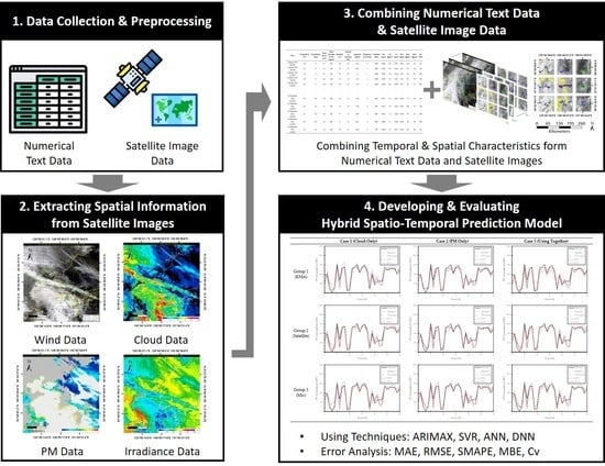
Research Framework
2. Methodology
2.1. Numerical Text Data
2.2. Satellite Image Data
2.2.1. Atmospheric Motion Vector (AMV) Image
2.2.2. Cloud Optical Thickness, Aerosol Optical Depth, and Insolation Image
2.3. Correlation Analysis with the Wind Direction of the Cloud and PM
| Algorithm 1. Algorithm of discriminant for movement of clouds and PM by wind direction. | |
| Denotes ; ; ; ; . | |
| 1: | Determination of by identification of in the |
| 2: | |
| 3: | Determination of the through |
| 4: | |
| 5: | Initialize the time step |
| 6: | Comparison of the amount of cloud in at and the amount of cloud in the |
| 7: | Comparison of the amount of cloud in and |
| 8: | For to |
| 9: | If |
| 10: | If |
| 11: | True |
| 12: | Else |
| 13: | False |
| 14: | Else |
| 15: | If |
| 16: | True |
| 17: | Else |
| 18: | False |
| 19: | |
3. Forecasting Method of Solar PV Generation
3.1. Prediction of Cloud and PM in ROI
3.2. Proposed Models for the Prediction of Solar PV Generation in ROI
3.2.1. Autoregressive Moving Integrated Average Exogenous input (ARIMAX)
3.2.2. Support Vector Regression (SVR)
3.2.3. Artificial Neural Network (ANN)
3.2.4. Deep Neural Network (DNN)
3.3. Analytic Process for Predicting Solar PV Generation
4. Results and Discussion
5. Conclusions
Author Contributions
Funding
Conflicts of Interest
References
- Cullen, D. Climate change. Nature 2011, 479, 267–268. [Google Scholar] [CrossRef]
- Horowitz, C.A. Paris Agreement. Int. Leg. Mater. 2016, 55, 740–755. [Google Scholar] [CrossRef]
- Ministry of Trade, Industry and Energy. Renewable Energy 3020 Plan. 3020 Plan; Ministry of Trade, Industry and Energy: Sejong, Korea, 2017.
- Korea Ministry of Trade, Industry and Energy. Renewable Energy Statistics 2013. 2014. Available online: http://www.motie.go.kr (accessed on 17 December 2017).
- Choi, H.; Zhao, W.; Ciobotaru, M.; Agelidis, V.G. Large-scale PV system based on the multiphase isolated DC/DC converter. In Proceedings of the 2012 3rd IEEE International Symposium on Power Electronics for Distributed Generation Systems (PEDG), Aalborg, Denmark, 25–28 June 2012; pp. 801–807. [Google Scholar] [CrossRef]
- Javier, M.; Luis, M.; Eduardo, L.; David, A.; Izco, E. Power output fluctuations in large scale PV plants: One year observations with one second resolution anda derived analytic model. Prog. Photovolt. 2011, 19, 218–227. [Google Scholar]
- Won, J.-M.; Doe, G.-Y.; Heo, N.-R. Predict Solar Radiation According to Weather Report. J. Korean Navig. Port Res. 2011, 35, 387–392. [Google Scholar] [CrossRef]
- Fang, X.; Misra, S.; Xue, G.; Yang, D. Smart Grid—The New and Improved Power Grid: A Survey. IEEE Commun. Surv. Tutor. 2011, 14, 944–980. [Google Scholar] [CrossRef]
- Bae, K.Y.; Jang, H.S.; Sung, D.K. Hourly Solar Irradiance Prediction Based on Support Vector Machine and Its Error Analysis. IEEE Trans. Power Syst. 2016, 32, 935–945. [Google Scholar] [CrossRef]
- Shi, J.; Lee, W.-J.; Liu, Y.; Yang, Y.; Wang, P. Forecasting Power Output of Photovoltaic Systems Based on Weather Classification and Support Vector Machines. IEEE Trans. Ind. Appl. 2012, 48, 1064–1069. [Google Scholar] [CrossRef]
- Yang, H.-T.; Huang, C.-M.; Huang, Y.-C.; Pai, Y.-S. A Weather-Based Hybrid Method for 1-Day Ahead Hourly Forecasting of PV Power Output. IEEE Trans. Sustain. Energy 2014, 5, 917–926. [Google Scholar] [CrossRef]
- Lee, D.; Kim, K. Deep Learning Based Prediction Method of Long-term Photovoltaic Power Generation Using Meteorological and Seasonal Information. Soc. e-Bus. Stud. 2019, 24, 1–16. [Google Scholar]
- Lee, K.; Kim, W.-J. Forecasting of 24_hours Ahead Photovoltaic Power Output Using Support Vector Regression. J. Korean Inst. Inf. Technol. 2016, 14, 175–183. [Google Scholar] [CrossRef]
- Jang, H.S.; Bae, K.Y.; Park, H.-S.; Sung, D.K. Solar Power Prediction Based on Satellite Images and Support Vector Machine. IEEE Trans. Sustain. Energy 2016, 7, 1255–1263. [Google Scholar] [CrossRef]
- Jang, H.S.; Bae, K.Y.; Park, H.-S.; Sung, D.K. Effect of aggregation for multi-site photovoltaic (PV) farms. In Proceedings of the 2015 IEEE International Conference on Smart Grid Communications (SmartGridComm), Miami, FL, USA, 2–5 November 2015; pp. 623–628. [Google Scholar] [CrossRef]
- Hammer, A.; Heinemann, D.; Lorenz, E.; Lückehe, B. Short-Term Forecasting of Solar Radiation. 1999 ISES Sol. World Congr. 2000, 67, 411–418. [Google Scholar] [CrossRef]
- Peng, Z.; Yoo, S.; Yu, D.; Huang, D. Solar irradiance forecast system based on geostationary satellite. In Proceedings of the 2013 IEEE International Conference on Smart Grid Commun. SmartGridComm, Vancouver, BC, Canada, 21–24 October 2013; pp. 708–713. [Google Scholar] [CrossRef]
- Kim, I.-J.; Lee, S.-K. A Study on the Design of Testable CAM using MTA Code. Trans. Korean Inst. Electr. Eng. 2019, 106–111. [Google Scholar] [CrossRef]
- Zhang, X.; Li, Y.; Lu, S.; Hamann, H.F.; Hodge, B.-M.; Lehman, B. A Solar Time Based Analog Ensemble Method for Regional Solar Power Forecasting. IEEE Trans. Sustain. Energy 2018, 10, 268–279. [Google Scholar] [CrossRef]
- Kang, H. An Analysis of the Causes of Fine Dust in Korea Considering Spatial Correlation. Environ. Resour. Econ. Rev. 2019, 28, 327–354. [Google Scholar] [CrossRef]
- Peters, I.M.; Karthik, S.; Liu, H.; Buonassisi, T.; Nobre, A. Urban haze and photovoltaics. Energy Environ. Sci. 2018, 11, 3043–3054. [Google Scholar] [CrossRef]
- Darwish, Z.A.; Kazem, H.A.; Sopian, K.; Al-Goul, M.; Alawadhi, H. Effect of dust pollutant type on photovoltaic performance. Renew. Sustain. Energy Rev. 2015, 41, 735–744. [Google Scholar] [CrossRef]
- Maghami, M.R.; Hizam, H.; Gomes, C.; Hajighorbani, S.; Rezaei, N. Evaluation of the 2013 Southeast Asian Haze on Solar Generation Performance. PLoS ONE 2015, 10, e0135118. [Google Scholar] [CrossRef]
- Sarver, T.; Al-Qaraghuli, A.; Kazmerski, L.L. A comprehensive review of the impact of dust on the use of solar energy: History, investigations, results, literature, and mitigation approaches. Renew. Sustain. Energy Rev. 2013, 22, 698–733. [Google Scholar] [CrossRef]
- Bergin, M.H.; Ghoroi, C.; Dixit, D.; Schauer, J.J.; Shindell, D. Large Reductions in Solar Energy Production Due to Dust and Particulate Air Pollution. Environ. Sci. Technol. Lett. 2017, 4, 339–344. [Google Scholar] [CrossRef]
- El-Shobokshy, M.S.; Hussein, F.M. Degradation of photovoltaic cell performance due to dust deposition on to its surface. Renew. Energy 1993, 3, 585–590. [Google Scholar] [CrossRef]
- Korea Meteorolgical Administration. Available online: https://data.kma.go.kr/ (accessed on 22 October 2020).
- Air Korea. Available online: https://www.airkorea.or.kr/ (accessed on 22 October 2020).
- Open Data Portal. Available online: https://www.data.go.kr/ (accessed on 22 October 2020).
- National Meteorological Satellite Center. Available online: https://nmsc.kma.go.kr/ (accessed on 22 October 2020).
- National Meteorological Satellite Center. AMV (AMV: Atmospheric Motion Vector) Algorithm Theoretical Basis Document; National Meteorological Satellite Center: Jincheon, Korea, 2012.
- National Meteorological Satellite Center. COT Algorithm Theoretical Basis Document; National Meteorological Satellite Center: Jincheon, Korea, 2012.
- National Meteorological Satellite Center. AOD Algorithm Theoretical Basis Document; National Meteorological Satellite Center: Jincheon, Korea, 2012.
- National Meteorological Satellite Center. INS Algorithm Theoretical Basis Document; National Meteorological Satellite Center: Jincheon, Korea, 2012.
- Wolff, B.; Kühnert, J.; Lorenz, E.; Kramer, O.; Heinemann, D. Comparing support vector regression for PV power forecasting to a physical modeling approach using measurement, numerical weather prediction, and cloud motion data. Sol. Energy 2016, 135, 197–208. [Google Scholar] [CrossRef]
- Li, L.; Gong, J.; Zhou, J. Spatial Interpolation of Fine Particulate Matter Concentrations Using the Shortest Wind-Field Path Distance. PLoS ONE 2014, 9, e96111. [Google Scholar] [CrossRef] [PubMed]
- Newsham, G.R.; Birt, B.J. Building-level occupancy data to improve ARIMA-based electricity use forecasts. In Proceedings of the 2nd ACM Workshop on Embedded Sensing Systems for Energy-Efficiency in Building, Zurich, Switzerland, 3–5 November 2010; pp. 13–18. [Google Scholar] [CrossRef]
- Dong-hyun, L.; A-hyun, J.; Jin-young, K.; Chang-Ki, K.; Hyun-goo, K.; Yung-seop, L. Solar Power Generation Forecast Model Using Seasonal ARIMA. Korean Sol. Energy Soc. 2019, 39, 59–66. [Google Scholar]
- Paulescu, M.; Badescu, V.; Brabec, M. Tools for PV (photovoltaic) plant operators: Nowcasting of passing clouds. Energy 2013, 54, 104–112. [Google Scholar] [CrossRef]
- Alsharif, M.H.; Younes, M.K.; Kim, J. Time Series ARIMA Model for Prediction of Daily and Monthly Average Global Solar Radiation: The Case Study of Seoul, South Korea. Symmetry 2019, 11, 240. [Google Scholar] [CrossRef]
- Cortes, C.; Vapnik, V. Support-vector networks. Mach. Learn. 1995, 20, 273–297. [Google Scholar] [CrossRef]
- Liu, W.; Liu, C.; Lin, Y.; Ma, L.; Xiong, F.; Li, J. Ultra-Short-Term Forecast of Photovoltaic Output Power under Fog and Haze Weather. Energies 2018, 11, 528. [Google Scholar] [CrossRef]
- Kim, K.; Jin, H. Photovoltaic Power Forecasting and Analysis of Forecasting Error for Model Learning Periods Using SVR. In Proceedings of the Korean Institute of Electrical Engineers, Pyeongchang, Korea, 11–13 July 2018; pp. 324–325. [Google Scholar]
- McCulloch, W.; Pitts, W. A logical calculus of the ideas immanent in nervous activity. Bull. Math. Biol. 1990, 52, 99–115. [Google Scholar] [CrossRef]
- Saberian, A.; Hizam, H.; Radzi, M.A.M.; Ab Kadir, M.Z.A.; Mirzaei, M. Modelling and Prediction of Photovoltaic Power Output Using Artificial Neural Networks. Int. J. Photoenergy 2014, 2014, 1–10. [Google Scholar] [CrossRef]
- Teoh, E.J.; Tan, K.C.; Xiang, C. Estimating the Number of Hidden Neurons in a Feedforward Network Using the Singular Value Decomposition. IEEE Trans. Neural Netw. 2006, 17, 1623–1629. [Google Scholar] [CrossRef]
- Liu, W.; Wang, Z.; Liu, X.; Zeng, N.; Liu, Y.; Alsaadi, F.E. A survey of deep neural network architectures and their applications. Neurocomputing 2017, 234, 11–26. [Google Scholar] [CrossRef]
- Oh, I.-S. Machine Learning; HANBIT Academy, Inc.: Seoul, Korea, 2017. [Google Scholar]
- ANSI/ASHRAE. ASHRAE Guideline 14-2002 Measurement of Energy and Demand Savings. ASHRAE 2002, 8400, 170. [Google Scholar]


| Date | Temperature [°C] | Precipitation [mm] | Wind Speed [m/s] | Wind Direction [0–360 degree] | Humidity [%] | Amount of Sunshine [hr] | Irradiance [MJ/m] | Cloudiness [0–10 level] | Visibility [10m] | SO2 [ppm] | CO [μg/m2] | O3 [ppm] | NO2 [ppm] | PM10 [μg/m2] | PM2.5 [μg/m2] | PV [kW] |
|---|---|---|---|---|---|---|---|---|---|---|---|---|---|---|---|---|
| 1 January 2015 09:00:00 | −8.4 | 0 | 6.7 | 340 | 56 | 0.8 | 0.21 | 0 | 2000 | 0.006 | 0.5 | 0.017 | 0.012 | 145 | 33 | 60 |
| 1 January 2015 10:00:00 | −8.1 | 0 | 6.1 | 226 | 54 | 0.0 | 0.67 | 1 | 2000 | 0.006 | 0.5 | 0.019 | 0.01 | 117 | 34 | 374 |
| 1 January 2015 11:00:00 | −7.6 | 0 | 6.1 | 340 | 53 | 0.0 | 1.1 | 1 | 2000 | 0.006 | 0.6 | 0.019 | 0.01 | 98 | 33 | 638 |
| 1 January 2015 12:00:00 | −6.9 | 0 | 6.4 | 340 | 52 | 0.0 | 1.41 | 1 | 2000 | 0.006 | 0.6 | 0.021 | 0.01 | 90 | 30 | 784 |
| 1 January 2015 12:00:00 | −6.1 | 0 | 6.4 | 340 | 53 | 0.0 | 1.53 | 1 | 2000 | 0.006 | 0.6 | 0.023 | 0.01 | 85 | 27 | 842 |
| . | . | . | . | . | . | . | . | . | . | . | . | . | . | . | . | . |
| . | . | . | . | . | . | . | . | . | . | . | . | . | . | . | . | . |
| . | . | . | . | . | . | . | . | . | . | . | . | . | . | . | . | . |
| 31 December 2015 13:00:00 | 2.9 | 0.0 | 3.3 | 360 | 74 | 1.0 | 1.38 | 4 | 800 | 0.011 | 1.2 | 0.013 | 0.042 | 78 | 66 | 230 |
| 31 December 2015 14:00:00 | 3.3 | 0.0 | 3.1 | 360 | 75 | 1.0 | 1.24 | 3 | 800 | 0.011 | 1.2 | 0.023 | 0.032 | 100 | 72 | 310 |
| 31 December 2015 15:00:00 | 3.1 | 0.0 | 3.4 | 340 | 77 | 1.0 | 0.93 | 3 | 800 | 0.011 | 1.2 | 0.024 | 0.034 | 87 | 67 | 439 |
| 31 December 2015 16:00:00 | 3.3 | 0.0 | 3.2 | 340 | 77 | 1.0 | 0.67 | 2 | 900 | 0.009 | 1.2 | 0.024 | 0.035 | 90 | 68 | 303 |
| 31 December 2015 17:00:00 | 2.9 | 0.0 | 2.1 | 320 | 78 | 1.0 | 0.26 | 0 | 700 | 0.009 | 1.2 | 0.017 | 0.047 | 83 | 65 | 95 |
| Channel | Center Wavelength (μm) | Wavelength Band (μm) | Spatial Resolution (km) |
|---|---|---|---|
| Visible | 0.67 | 0.55~0.8 | 1 |
| Shortwave Infrared | 3.7 | 3.5~4.0 | 4 |
| Water vapor | 6.7 | 6.5~7.0 | 4 |
| Infrared 1 | 10.8 | 10.3~11.3 | 4 |
| Infrared 2 | 12.0 | 11.5~12.5 | 4 |
| Date | Wind Direction | Clear | Partly Cloudy | Mostly Cloudy | Cloudy |
|---|---|---|---|---|---|
| 18 January 2015 11:00:00 | W | 0 | 0 | 0 | 0 |
| 18 January 2015 12:00:00 | W | 1608 | 114 | 6 | 0 |
| 18 January 2015 13:00:00 | SW | 1147 | 935 | 31 | 0 |
| 18 January 2015 14:00:00 | W | 0 | 0 | 0 | 0 |
| 2015-08-02 08:00:00 | SW | 0 | 0 | 0 | 0 |
| 2015-08-02 09:00:00 | W | 175 | 636 | 165 | 6 |
| 2015-08-02 10:00:00 | W | 238 | 332 | 222 | 35 |
| 2015-08-02 11:00:00 | W | 52 | 591 | 364 | 0 |
| Date | Wind Direction | Good | Moderate | Unhealthy | Very Unhealthy |
|---|---|---|---|---|---|
| 18 January 2015 11:00:00 | W | 27 | 131 | 119 | 57 |
| 18 January 2015 12:00:00 | W | 0 | 88 | 204 | 78 |
| 18 January 2015 13:00:00 | SW | 0 | 4 | 30 | 20 |
| 18 January 2015 14:00:00 | W | 0 | 6 | 0 | 0 |
| 2 August 2015 08:00:00 | SW | 6 | 144 | 12 | 18 |
| 2 August 2015 09:00:00 | W | 0 | 12 | 12 | 9 |
| 2 August 2015 10:00:00 | W | 0 | 9 | 62 | 39 |
| 2 August 2015 11:00:00 | W | 0 | 0 | 0 | 18 |
| Cloud | Clear | Partly Cloudy | Mostly Cloudy | Cloudy |
|---|---|---|---|---|
| Accuracy (%) | 75.068 | 75.793 | 84.044 | 91.296 |
| PM | Good | Moderate | Unhealthy | Very Unhealthy |
|---|---|---|---|---|
| Accuracy (%) | 87.489 | 85.585 | 89.665 | 93.382 |
| Number of Hidden Layer | 1 | 2 | 3 | 4 | 5 | 6 | 7 |
|---|---|---|---|---|---|---|---|
| Number of Nodes | 180 | 0.4 | 100 | 0.4 | 100 | 0.4 | 1 |
| Activation Function | tanh | Drop out | Relu | Drop Out | Sigmoid | Drop out | Sigmoid |
| Group 1 (Numerical Text Weather Data) | Group 2 (Satellite Images) | Group 3 (Mixed, G1 + G2) | |
|---|---|---|---|
| Common Parameters | Month, Day, Time, PV (previous data) | ||
| Case 1 (Cloud) | Temperature, Precipitation, Wind Speed, Wind Direction, Humidity, Amount of Sunshine, Irradiance, Cloudiness, Visibility | Wind Speed, Wind Direction, Clear, Partly cloudy, Mostly cloudy, Cloudy, Irradiance | Temperature, Precipitation, Wind Speed, Wind Direction, Humidity, Amount of Sunshine, Irradiance, Clear, Partly cloudy, Mostly cloudy, Cloudy, Visibility |
| Case 2 (PM) | Temperature, Precipitation, Wind Speed, Wind Direction, Humidity, Amount of Sunshine, Irradiance, SO2, CO, O3, NO2, PM10, PM2.5, Visibility | Wind Speed, Wind Direction, PM_Good, PM_Moderate, PM_Unhealthy, PM_Very Unhealthy, Irradiance | Temperature, Precipitation, Wind Speed, Wind Direction, Humidity, Amount of Sunshine, Irradiance, PM_Good, PM_Moderate, PM_Unhealthy, PM_Very Unhealthy, Visibility |
| Case 3 (Cloud + PM) | Temperature, Precipitation, Wind Speed, Wind Direction, Humidity, Amount of Sunshine, Irradiance, SO2, CO, O3, NO2, PM10, PM2.5, Cloudiness, Visibility | Wind Speed, Wind Direction, Clear, Partly cloudy, Mostly cloudy, Cloudy, PM_Good, PM_Moderate, PM_Unhealthy, PM_Very Unhealthy, Irradiance | Temperature, Precipitation, Wind Speed, Wind Direction, Humidity, Amount of Sunshine, Irradiance, Clear, Partly cloudy, Mostly cloudy, Cloudy, PM_Good, PM_Moderate, PM_Unhealthy, PM_Very Unhealthy, Visibility |
| Output Parameter | PV (One hour ahead) | ||
| Calibration Type | Index | Acceptable Value |
|---|---|---|
| Monthly | MBE month | ± 5% |
| Cv (RMSE) month | 15% | |
| Hourly | MBE hour | ±10% |
| Cv (RMSE) hour | 30% |
| Group | Error | ARIMIX | SVR_RBF | SVR_Linear | SVR_Poly | ANN | DNN |
|---|---|---|---|---|---|---|---|
| Group 1 (Numerical Text Data) | MAE | 81.261 | 90.686 | 81.112 | 102.638 | 122.285 | 72.554 |
| RMSE | 101.768 | 111.289 | 101.63 | 128.766 | 149.354 | 98.519 | |
| SMAPE | 17.845 | 17.114 | 17.91 | 21.16 | 19.706 | 14.197 | |
| MBE | 0.017 | 0.394 | 0.526 | 0.504 | 23.958 | 0.956 | |
| Cv | 22.593 | 24.706 | 22.562 | 28.587 | 33.157 | 21.872 | |
| Group 2 (Satellite Images) | MAE | 79.186 | 101.178 | 81.147 | 180.107 | 92.738 | 73.496 |
| RMSE | 101.712 | 124.462 | 103.107 | 232.476 | 117.635 | 95.934 | |
| SMAPE | 15.635 | 18.178 | 16.51 | 28.447 | 16.786 | 14.484 | |
| MBE | 0.093 | 0.052 | 0.455 | 12.666 | 13.171 | 3.142 | |
| Cv | 22.58 | 27.631 | 22.89 | 51.61 | 26.115 | 21.298 | |
| Group 3 (Mixed, G1 + G2) | MAE | 78.143 | 88.868 | 78.884 | 85.339 | 92.323 | 67.531 |
| RMSE | 101.496 | 109.402 | 100.88 | 116.526 | 114.274 | 93.642 | |
| SMAPE | 17.792 | 16.841 | 17.613 | 16.58 | 17.857 | 15.039 | |
| MBE | 0.06 | 0.592 | 0.14 | 3.89 | 12.21 | 6.013 | |
| Cv | 22.532 | 24.288 | 22.396 | 25.869 | 25.369 | 20.789 |
| Group | Error | ARIMIX | SVR_RBF | SVR_Linear | SVR_Poly | ANN | DNN |
|---|---|---|---|---|---|---|---|
| Group 1 (Numerical Text Data) | MAE | 79.753 | 94.812 | 83.152 | 76.808 | 86.44 | 75.432 |
| RMSE | 100.344 | 115.05 | 104.319 | 97.71 | 106.326 | 95.944 | |
| SMAPE | 17.377 | 17.417 | 18 | 16.241 | 19.124 | 14.439 | |
| MBE | 0.265 | 1.8 | 1.301 | 1.585 | 10.807 | 3.661 | |
| Cv | 22.277 | 25.541 | 23.159 | 21.692 | 23.605 | 21.3 | |
| Group 2 (Satellite Images) | MAE | 78.33 | 96.5 | 78.103 | 190.973 | 82.34 | 75.727 |
| RMSE | 102.158 | 118.679 | 99.672 | 255.323 | 105.741 | 103.094 | |
| SMAPE | 16.683 | 17.757 | 17.017 | 28.403 | 15.489 | 15.202 | |
| MBE | 0.106 | 1.665 | 0.009 | 18.586 | 3.51 | 0.303 | |
| Cv | 22.679 | 26.347 | 22.127 | 56.682 | 23.475 | 22.887 | |
| Group 3 (Mixed, G1 + G2) | MAE | 78.895 | 90.663 | 80.282 | 77.882 | 93.974 | 71.295 |
| RMSE | 102.432 | 110.424 | 102.413 | 104.554 | 115.703 | 96.355 | |
| SMAPE | 17.631 | 16.957 | 18.229 | 15.217 | 17.829 | 14.257 | |
| MBE | 0.195 | 0.493 | 0.482 | 1.207 | 12.481 | 2.156 | |
| Cv | 22.74 | 24.514 | 22.736 | 23.211 | 25.686 | 21.391 |
| Group | Error | ARIMIX | SVR_RBF | SVR_Linear | SVR_Poly | ANN | DNN |
|---|---|---|---|---|---|---|---|
| Group 1 (Numerical Text Data) | MAE | 196.129 | 90.096 | 81.154 | 79.128 | 95.97 | 79 |
| RMSE | 235.048 | 111.22 | 102.268 | 100.929 | 119.607 | 104.059 | |
| SMAPE | 31.626 | 17.041 | 17.596 | 16.49 | 20.808 | 15.123 | |
| MBE | 11.816 | 2.076 | 0.171 | 1.219 | 6.619 | 8.376 | |
| Cv | 52.181 | 24.691 | 22.704 | 22.406 | 26.553 | 23.101 | |
| Group 2 (Satellite Images) | MAE | 78.444 | 93.155 | 81.448 | 126.299 | 82.911 | 77.713 |
| RMSE | 100.831 | 115.8223 | 102.696 | 169.343 | 107.843 | 102.005 | |
| SMAPE | 15.783 | 17.539 | 17.04 | 21.657 | 16.08 | 14.815 | |
| MBE | 0.146 | 0.883 | 0.744 | 4.915 | 8.321 | 5.343 | |
| Cv | 22.385 | 25.713 | 22.799 | 37.604 | 23.941 | 22.646 | |
| Group 3 (Mixed, G1 + G2) | MAE | 77.554 | 87.587 | 80.123 | 83.163 | 101.233 | 71.532 |
| RMSE | 101.943 | 108.229 | 102.889 | 107.278 | 122.508 | 92.938 | |
| SMAPE | 17.669 | 16.66 | 17.91 | 17.373 | 18.776 | 14.107 | |
| MBE | 0.342 | 0.498 | 0.039 | 0.134 | 16.572 | 4.986 | |
| Cv | 22.632 | 24.027 | 22.842 | 23.816 | 27.197 | 20.633 |
| Case 1 (Cloud Only) | Case 2 (PM Only) | Case 3 (Using Together) | |
|---|---|---|---|
| Group 1 (KMA) |  |  |  |
| Group 2 (Satellite) |  |  |  |
| Group 3 (Mix) |  |  |  |
Publisher’s Note: MDPI stays neutral with regard to jurisdictional claims in published maps and institutional affiliations. |
© 2020 by the authors. Licensee MDPI, Basel, Switzerland. This article is an open access article distributed under the terms and conditions of the Creative Commons Attribution (CC BY) license (http://creativecommons.org/licenses/by/4.0/).
Share and Cite
Kim, B.; Suh, D. A Hybrid Spatio-Temporal Prediction Model for Solar Photovoltaic Generation Using Numerical Weather Data and Satellite Images. Remote Sens. 2020, 12, 3706. https://doi.org/10.3390/rs12223706
Kim B, Suh D. A Hybrid Spatio-Temporal Prediction Model for Solar Photovoltaic Generation Using Numerical Weather Data and Satellite Images. Remote Sensing. 2020; 12(22):3706. https://doi.org/10.3390/rs12223706
Chicago/Turabian StyleKim, Bowoo, and Dongjun Suh. 2020. "A Hybrid Spatio-Temporal Prediction Model for Solar Photovoltaic Generation Using Numerical Weather Data and Satellite Images" Remote Sensing 12, no. 22: 3706. https://doi.org/10.3390/rs12223706
APA StyleKim, B., & Suh, D. (2020). A Hybrid Spatio-Temporal Prediction Model for Solar Photovoltaic Generation Using Numerical Weather Data and Satellite Images. Remote Sensing, 12(22), 3706. https://doi.org/10.3390/rs12223706