Article

An Improved Spatiotemporal Data Fusion Method Using Surface Heterogeneity Information Based on ESTARFM

1
State Key Laboratory of Earth Surface Processes and Resource Ecology, Beijing Normal University, Beijing 100875, China
2
Faculty of Geographical Science, Beijing Normal University, Beijing 100875, China
3
College of Resources Science and Technology, Beijing Normal University, Beijing 100875, China
4
School of Information Engineering, China University of Geosciences, Beijing 100083, China
5
College of Resources and Environmental Sciences, Henan Agricultural University, Zhengzhou 450002, China
*
Author to whom correspondence should be addressed.
Remote Sens. 2020, 12(21), 3673; https://doi.org/10.3390/rs12213673
Submission received: 6 October 2020 / Revised: 31 October 2020 / Accepted: 7 November 2020 / Published: 9 November 2020

Abstract

:
The use of the spatiotemporal data fusion method as an effective data interpolation method has received extensive attention in remote sensing (RS) academia. The enhanced spatial and temporal adaptive reflectance fusion model (ESTARFM) is one of the most famous spatiotemporal data fusion methods, as it is widely used to generate synthetic data. However, the ESTARFM algorithm uses moving windows with a fixed size to get the information around the central pixel, which hampers the efficiency and precision of spatiotemporal data fusion. In this paper, a modified ESTARFM data fusion algorithm that integrated the surface spatial information via a statistical method was developed. In the modified algorithm, the local variance of pixels around the central one was used as an index to adaptively determine the window size. Satellite images from two regions were acquired by employing the ESTARFM and modified algorithm. Results showed that the images predicted using the modified algorithm obtained more details than ESTARFM, as the frequency of pixels with the absolute difference of mean value of six bands’ reflectance between true observed image and predicted between 0 and 0.04 were 78% by ESTARFM and 85% by modified algorithm, respectively. In addition, the efficiency of the modified algorithm improved and the verification test showed the robustness of the modified algorithm. These promising results demonstrated the superiority of the modified algorithm to provide synthetic images compared with ESTARFM. Our research enriches the spatiotemporal data fusion method, and the automatic selection of moving window strategy lays the foundation of automatic processing of spatiotemporal data fusion on a large scale.

Graphical Abstract

1. Introduction

Recently, remote sensing has become a universal technology to monitor dynamic changes of resources and the environment [1]. The spatiotemporal heterogeneity, spatiotemporal correlation, and scale characteristics of geographical phenomena pose great challenges to the monitoring and analytical methods of remote sensing. Due to the limitation of the satellite revisit period, tradeoff between scanning swath and pixel size of sensor, observation condition (cloudy and rainy), and other reasons, it is difficult to simultaneously obtain images with high temporal and spatial resolution. Fortunately, spatiotemporal data fusion methods have received extensive attention [2] in remote sensing studies because of its capability to generate images with high spatiotemporal resolution images from frequent coarse resolution images and sparse fine resolution images [3]. It is a flexible, inexpensive and effective solution to cover the data shortage problem in some situations. Spatiotemporal data fusion methods have been applied to generate synthetic remote sensing imagery from multiple sources with different spatial, temporal, and spectral characteristics, and the fused results can convey more abundant and accurate information than individual sensors alone [4]. Spatiotemporal data fusion methods can provide data foundation for remote sensing field such as environmental dynamic monitoring [5,6], changes of land cover [7], and land surface temperature [4,8].
There are many spatiotemporal data fusion methods in the remote sensing field. These methods are based on different principles, assumptions, and strategies. According to Zhu et al. [9], spatiotemporal data fusion methods can be divided into five categories: unmixing-based methods [10,11,12], weighted function-based methods [7,13,14], Bayesian-based methods [15,16,17], learning-based methods [18,19,20], and hybrid methods [21,22,23]. Among these methods, the weighted function-based methods are most widely used in practical applications, while the spatial and temporal adaptive reflectance fusion model (STARFM) [24] was put forward first and gained popularity in generating remote sensing data [25,26]. However, STARFM has some constraints in practical applications. It cannot predict the changing information that is not recorded in based images. Moreover, it cannot obtain good performance in highly heterogeneous regions. Furthermore, it does not take the bidirectional reflectance distribution function problem into consideration. Several improved algorithms have been developed to mitigate these problems. The spatial temporal adaptive algorithm for mapping reflectance change (STAARCH) use tasseled cap transformations of input data to detect disturbances [27]. The enhanced spatial and temporal adaptive reflectance fusion model (ESTARFM) was developed to improve STARFM accuracy in heterogeneous areas by introducing a conversion coefficient and temporal weight of input image pairs [28]. The STARFM was also improved to an operational data fusion framework by appending Bidirectional Reflectance Distribution Function (BRDF) correction, automatic co-registration, and input data selection [29]. Modified spatiotemporal fusion algorithms based on STARFM spring up because of the emergence of new satellite data (such as Sentinel) and data processing technology (deep learning) [30,31].
However, due to the algorithm design, all STARFM-based algorithms have two input control parameters: the number of land cover classes and the size of the moving window. The landscape and land cover types of the study area determine the size of the moving window. Most previous studies used 1500 m × 1500 m as the moving window size when fusing Landsat and MODIS data, which are similar to Gao’s work [24]. The overlapping moving window technique ensures that the most spectrally similar pixels are selected for the best interest of the central pixel [32]. Therefore, the size of the moving window is important for the performance of STARFM-based algorithms [33]. On the one hand, if the window size is too small, the algorithm cannot search the neighborhood pixels that are similar to the central pixel in the heterogeneity region. On the other hand, if the window size is too large, it may take massive noneffective calculations in the algorithm. Furthermore, a universal window in one satellite image size might not exist because of the inter-class and intra-class heterogeneity of land surface and the different degree of landscape heterogeneity. With increased spatiotemporal resolution, RS data becomes denser in the time scale, and data processing efficiency becomes increasingly important.
Hence, this paper concentrated on adopting an adaptive moving window in a spatiotemporal data fusion algorithm and introducing a spatial statistical method according to landscape heterogeneity. The adaptive moving window strategy in the spatiotemporal algorithm can reduce the redundancy and improve the efficiency of the algorithm. It is also conducive to remote sensing data reconstruction for long time series analysis. Therefore, this improvement using surface heterogeneity information not only promotes the performance of spatiotemporal data fusion algorithm but also lays the foundation of automatic processing on a large scale.

2. Materials

2.1. Study Area

In this paper, we studied two regions to verify the modified algorithm’s accuracy: study area A and study area B, respectively. As shown in Figure 1, study area A was located in Jiujiang, Jiangxi province, China (28°47′N~30°06′N, 113°57′E~116°53′E) while study area B was located in Langfang, Hebei province, China (39°28′N~39°32′N, 116°38′E~116°44′E). Jiujiang city is adjacent to Poyang Lake, which is the second largest lake and largest freshwater lake in China. Jiujiang is located in a subtropical monsoon climate zone. Jiujiang is relatively complex in terrain and landform. Langfang City is located in the mid-latitude zone, with a warm temperate continental monsoon climate with four distinct seasons. It has sufficient light and heat resources, with rain and heat in the same season, which is beneficial to crop growth.

2.2. Data

Landsat provided surface monitoring images for 40 years (1972-present) [34]. A large number of studies showed that spatial resolution of 30 m was well suited for regional-scale and long-term monitoring of surface changes [35,36]. However, with its 16-day return visit cycle and frequent cloud pollution problems, Landsat images were hard to apply to monitoring and analysis of short-period surface changes. MODIS images had stronger real-time monitoring capabilities for various sudden and rapidly changing natural disasters because of its less than one day revisit period. However, the spatial resolution of MODIS only reached 250 m. Landsat images are sparse fine-resolution images and MODIS images are frequent coarse-resolution images. Therefore, Landsat and MODIS images are suitable for spatiotemporal data fusion with complementary advantages. In this paper, Landsat 7 ETM+, Landsat 8 OLI, and MODIS data were employed to test ESTARFM and the modified algorithm. The bands of Landsat and corresponding bands of MODIS are listed in Table 1. It was inevitable that there were some differences between MODIS’s bands and corresponding bands of Landsat7 ETM+/Landsat8 OLI due to different sensor design.
Clear Landsat images showed that cloud cover was less than 10% and the MODIS eight-day composite reflectance data (MOD09A1) that avoided heavy cloud contamination were adopted to conduct data fusion algorithms. The Landsat images and their corresponding MODIS images that were selected in this study had four-day intervals. The MODIS images were clipped, re-projected, and resampled in order to keep consistent with Landsat images. The original reflectance images were scaled 0-10000. Two observed Landsat images of prediction date were selected to conduct an accuracy assessment with synthetic images. Relevant remote sensing data with their acquisition date and application are listed in Table 2.

3. Method

3.1. The Overview of ESTARFM

The main idea of ESTARFM is to obtain the reflectance at a predicted date based on spectral, temporal, and spatial information from input images at a base date. Its main contribution is to introduce conversion coefficients and temporal weight between input data pairs to minimize the system biases and improve accuracy. In order to predict the surface reflectance, the ESTARFM algorithm can be reduced to four steps: the selection of similar neighborhood pixels, the calculation of weights for similar pixels, the calculation of conversion coefficient, and the calculation of reflectance of the central pixel.
(1) The selection of similar neighborhood pixels. The similar neighborhood pixels contain important spectral and spatial information, which is the basis for predicting surface reflectance on a predicted date. The ESTARFM employs the threshold method to search for similar neighborhood pixels. The formula is as follows:
F x i , y i , t k , B F x w / 2 , y w / 2 , t k , B σ B × 2 / m
where F(xi,yi,tk,B) is fine resolution reflectance of neighborhood pixels at a base date(tk), F(xw/2,yw/2,tk,B) is fine resolution reflectance of central pixel at a base date(tk), σ(B) is the standard deviation of reflectance for band B, and m is the estimated number of class of land cover.
(2) The calculation of weights for similar pixels. The weight (Wi) is determined by the location of similar pixels and the spectral similarity between fine- and coarse-resolution pixels. Higher similarity and smaller distances of the similar pixels to the central pixels produce a higher weight.
(3) The calculation of conversion coefficient (Vi). The algorithm uses a linear regression model to acquire Vi from fine- and coarse-resolution reflectance of the similar pixels within the same coarse pixel to obtain conversion coefficients.
(4) The calculation of reflectance of the central pixel. The predicted reflectance of the center pixel is as follows:
F x w / 2 , y w / 2 , t p , B = F x w / 2 , y w / 2 , t 0 , B + i = 1 N W i × V i × C x i , y i , t p , B C x i , y i , t 0 , B
where C(xi,yi,tp,B) is the reflectance of similar pixel of band B at the prediction time of fine-resolution images and C(xi,yi,t0,B) is the reflectance of similar pixel of band B at a base time of coarse-resolution images.
In order to minimize the system biases, ESTARFM introduced a temporal weight to improve prediction and accuracy. Therefore, the final predicted fine-resolution reflectance at the prediction time tp is calculated as:
F x w / 2 , y w / 2 , t p , B = T m × F m x w / 2 , y w / 2 , t p , B + T n × F n x w / 2 , y w / 2 , t p ,   B
where Tm and Tn are the temporal weight between the time, Tm, and prediction, as well as temporal weight between time, Tn, and prediction, respectively.

3.2. The Proposed Methodology

According to Tobler’s first law of geography [37], everything is related but nearby things are more related [38]. Therefore, spatial dependence is a rule used by nearly all spatiotemporal data fusion algorithms. The introduction of moving a window strategy ensures that the most spectrally similar pixels are selected for the best interest of the central pixel. However, the surface landscape is heterogeneous, and ESTARFM use the fixed size moving window to search for similar pixels. For example, in a region with homogeneous surfaces, a fixed-size window may bring redundant calculations and reduce the efficiency of the spatiotemporal data fusion algorithm. If landscape heterogeneity is high, the number of selected similar pixels may not be enough within a fixed-size window. If we cannot obtain enough similar pixels when predicting the reflectance in the ESTARFM algorithm, linear regression cannot be built to obtain the conversion coefficients of similar pixels. If linear regression is not possible, ESTARFM directly uses reflectance of the center pixel on a base date to replace the reflectance of the center pixel on a prediction date. Therefore, the accuracy of the spatiotemporal data fusion algorithm is reduced. The fixed size moving window is not suitable when there is a difference in the heterogeneity of an image. Therefore, aiming at solving the fixed size of overlapping moving window, this paper proposed a new methodology to find the optimum size of a moving window for the center pixel by introducing an adaptive moving window strategy.

3.2.1. The Introduction of Local Variance

One of the biggest features of the landscape is spatial autocorrelation. Spatial autocorrelation means that the closer a thing or phenomenon in space is, the more similar they are, i.e., changes in landscape features or variables in the vicinity often show dependence on spatial location. Moreover, the spatial autocorrelation coefficient also varies when the observed scale changes. In the process of spatial autocorrelation analysis, it is better to calculate the autocorrelation coefficient on a series of different scales to reveal the degree of autocorrelation of the variable under the changes of the spatial scale in study. For the same reason, the spatial autocorrelation coefficient also varies within different moving window sizes. However, ESTARFM uses the same fixed-size moving window for the same image when the heterogeneity of an image is different. When the radius of the moving window is small, the features of the adjacent pixels in heterogeneous landscapes may not have a higher similarity with the features of target pixels than those of adjacent pixels, so less than enough similar pixels may be selected to participate in the linear regression of space-time fusion and have an impact on the prediction of pixel information. When the radius of the moving window is large, it not only results in an average of the reflectance change information of the spectral similar pixels in the window, but also may significantly increase the number of operations, especially in heterogeneous regions, which may lead to a large number of invalid operations. Therefore, moving window size is important for STARFM-based algorithm performance. Flexible moving window size can enable us to get reliable and enough information from surrounding pixels by selecting similar pixels of the center pixel in the spatiotemporal data fusion algorithm. Therefore, we introduced a mean local variance to search the most suitable moving window size in the spatiotemporal data fusion algorithm. The local variance (s2) is an index that measures the similarity of neighborhood pixels in remote sensing pixels. The function is as follows:
s 2 = i = 0 M 1 j = 0 N 1 f b i , j f b 2 M N ,
f b = i = 0 M 1 j = 0 N 1 f b i , j M N ,
where i and j are the horizontal and vertical positions of pixels in satellite image; fb (i, j) is the value of the reflectance of the center pixel of band b within the window; M and N represent the size of the moving window; and fb is the average reflectance value for pixels within the window. The mean local variance (S2mean) is calculated by averaging the local variance within the window.
S m e a n 2 = S 2 M N
The mean local variance is based on the difference of reflectance in neighborhood pixels, and it can reflect the characteristic scale of the landscape in remote sensing images.

3.2.2. The Calculation of Local Variance within Different Moving Windows

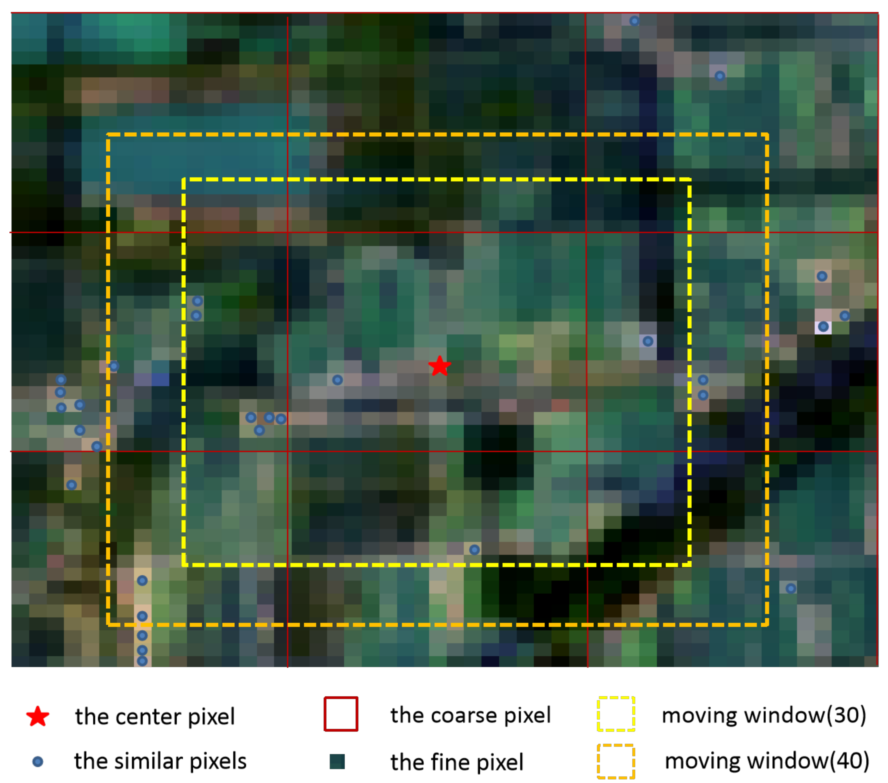
The mean local variance is based on the difference of values of adjacent pixels’ reflectance, which reflects the minimum characteristic scale affected by the landscape. In this paper, mean local variance index was introduced to indicate spatial heterogeneity in different window sizes. Local variance is an indicator of similarity between neighborhood pixels in remote sensing images; however, the mean local variance is different from the local variance. The window corresponding to the largest local variance can represent the optimal scale of the main land cover within the moving window, and the selected similar pixels are likely to come from the same type of land cover. Selected similar pixels can better reflect the central pixel’s information. Secondly, the window corresponding to the maximum local average variance can select an appropriate number of similar neighboring pixels to participate in the fusion, which can either reduce unnecessary calculations and improve spatiotemporal data fusion algorithm efficiency, or provide enough pixel information to improve fusion accuracy. Based on the center pixels in the moving window, the local variance index is calculated under different moving window sizes, then mean local variance index values can be obtained by averaging the local variance index under different moving window sizes. Figure 2 is a schematic diagram about the calculation of the mean local variance index in an adaptive moving window strategy in the spatiotemporal data fusion method. In Figure 2, the center pixel is the building and similar pixels in the neighborhood of the central pixel are marked by a blue circle. The yellow boxes represent the different sized moving windows and the average local variance in different sized moving windows, respectively. Finally, the window size corresponding to the maximum mean local variance is selected as the size of the window in spatiotemporal data fusion algorithm. In order to simplify the algorithm, the selection threshold of moving window size within the algorithm is 30 to150, the step length is 10, and the unit is Landsat pixel.

3.2.3. Carrying Out of Modified Algorithm

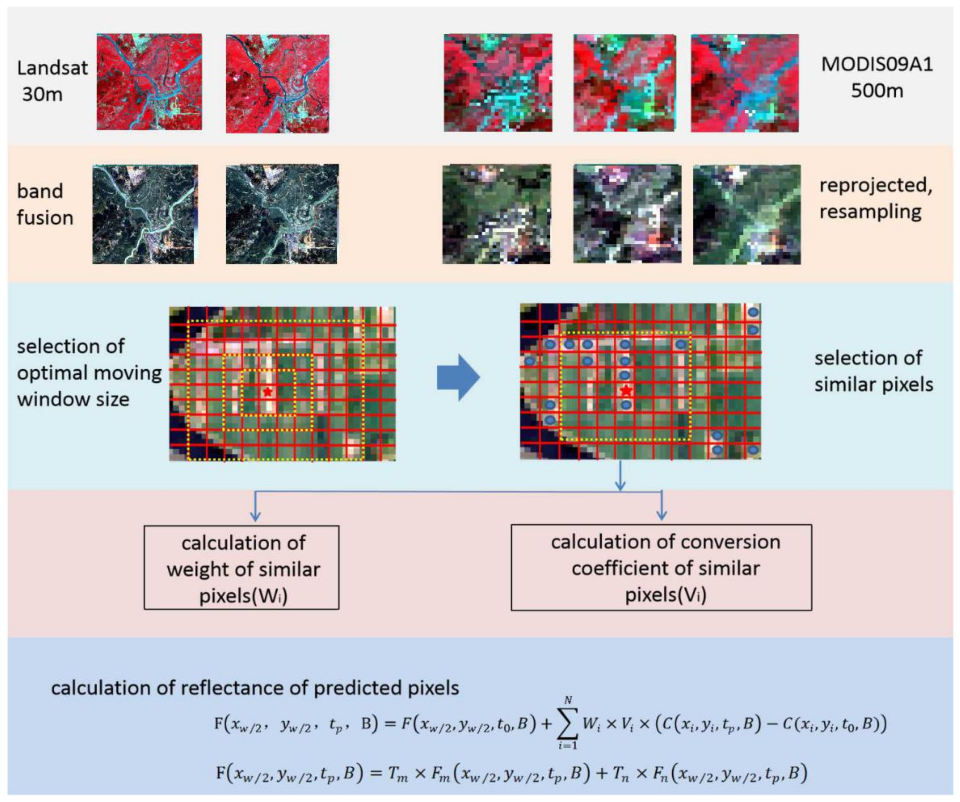
The implementation of the advanced algorithm includes data processing, the selection of optimal moving window size and similar pixels, the calculation of weight and conversion coefficient of similar pixels, and the calculation of predicted pixel reflectance. Data processing includes the processing of Landsat and MODIS09A1 data. Landsat data requires band composite and clipping. MODIS09A1 data needs to be re-projected, resampled, and clipped in MRT to maintain the same projection system and spatial resolution as Landsat data. For the selection of optimal moving window size and selection of similar pixels, mean local variances within 30*30 Landsat pixel size windows to 150*150 Landsat pixel size windows were respectively calculated in the neighborhood of the central pixel. Then, the size of the moving window corresponding to the largest local variance is taken as the moving window of the center pixel, and the similar pixel of the center pixel is found in this window. The rules for calculating the weight and conversion coefficient of similar pixels and reflectance of predicted pixels are the same as ESTARFM [28]. The algorithm flow is shown in Figure 3.

4. Results

4.1. Subjective Assessment

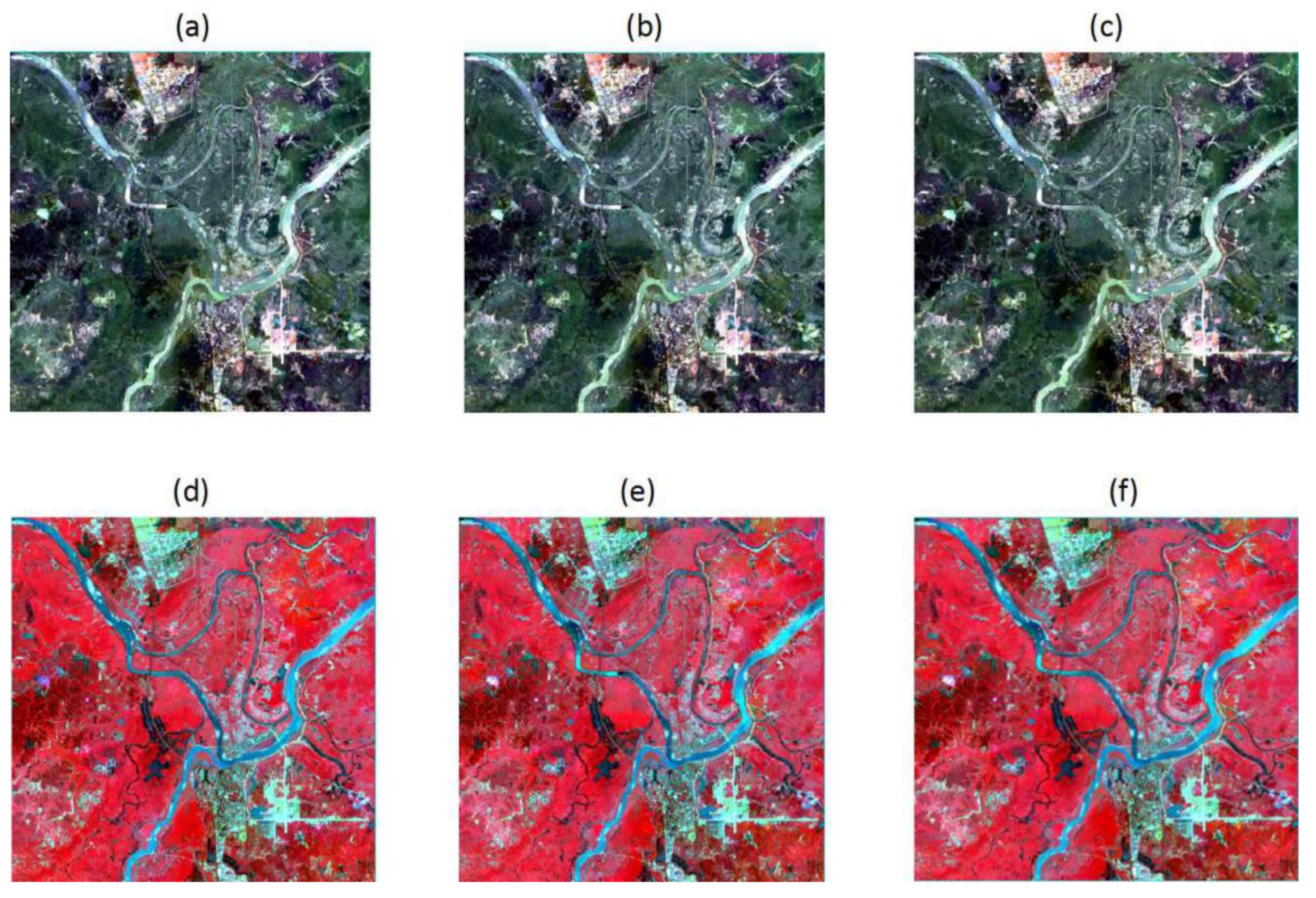
In order to obtain the prediction accuracy of the spatiotemporal data fusion algorithm based on surface spatial features, this study compared the result obtained by the modified algorithm, as well as the results obtained by ESTARFM and real images. The results are shown in Figure 4. Visually, ESTARFM and the modified algorithm both obtained good composite images, which were similar to the actual observed image. However, ESTARFMs original code and the modified algorithm were both written in the Interactive Data Language (IDL) language. The running time of the modified algorithm was reduced by half that of the ESTARFM when the same input images were processed in the same computer configuration.
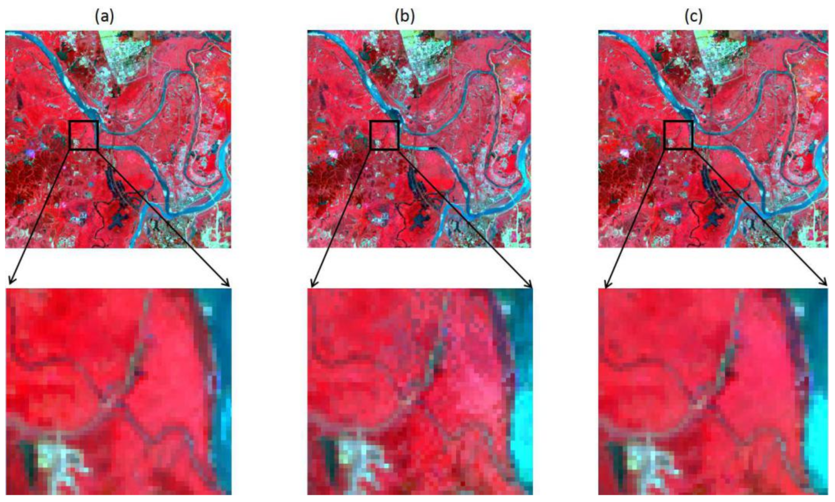
As shown in Figure 5, in the black box we observed a border of water, as well as vegetation and buildings. The shape of the river is unclear and the vegetation pixel is fuzzy around the river in the enlarged figure. The result predicted using the modified algorithm retained more detailed information and showed a clearer visual effect. However, the spatiotemporal data fusion algorithm based on the spatial structure information did not show good advantages in the regions with high surface homogeneity.

4.2. Objective Assessment

4.2.1. The Ordinary Indicator

Unlike our previous work [39], in this study the spatiotemporal data fusion algorithm using surface heterogeneity information based on ESTARFM oriented the entire image rather than concentrating on a type of land cover. Therefore, we observed all four main land cover types and evaluated each, i.e., buildings, water, paddy, and non-paddy vegetation. Moreover, the statistical analysis of six bands were carried out in order to obtain more accurate results. The regression coefficient of the linear fitting equation (ρ), correlation coefficient (r), and root mean square error (RMSE) were employed to compare the reflectance of the predicted image with the true observed image. The closer the value of ρ and r were to 1, the more accurate the result was. The smaller the RMSE value was, the better accuracy the results were.
Figure 6 shows the scatter plots along the 1:1 line of the observed reflectance values and estimated value for each band of ESTARFM and the modified algorithm. The left column of scatter plots are ESTARFM results and the right column are the modified algorithm results. From the results shown in Figure 6, we observed that the modified algorithm performed well in Bands 1–4 (i.e., blue, green, red, and NIR). For Band 5 (SWIR1), the accuracy of the two algorithm was almost the same. For Band 6 (SWIR2), ESTARFM obtained the better result.
Table 3 shows a quantitative comparison of each band for each land cover between the ESTARFM and modified algorithm. The better results of ESTARFM are highlighted in bold. It can be seen that different accuracy evaluation indexes of different surface features in different bands did not show a uniform rule. Most of the pixels in Band 6 (SWIR2) did not obtain better results in the modified algorithm than in the ESTARFM. Band 6 was a mid-infrared band, which was useful for mineral discrimination, and could be used to identify vegetation cover and moist soil. Hence, the modified algorithm was not suitable for rock and mineral discrimination. For other bands, although the modified algorithm obtained better performance than ESTARFM, the advantage of the modified algorithm were not obvious. However, the only one we ensured was that the modified algorithm was less than the ESTARFM, as mentioned above. In general, the subject assessment really verified that the results predicted by the modified algorithm were more effective than ESTARFM. However, the normal accuracy evaluation indexes may not be applicable for evaluating the overall accuracy of the spatiotemporal data fusion algorithm based on the spatial structure information of the surface.

4.2.2. The Mean Difference of Six Bands

As stated above, different selected evaluation indexes of different land cover types in different bands did not show a uniform rule and thus the evaluation indexes were not appropriate when evaluating the overall accuracy of the spatiotemporal data fusion algorithm based on the spatial structure information of the surface. Therefore, this paper put forth a mean difference of a six band reflectance [40,41] to measure the overall precision of the two spatiotemporal data fusion algorithms. Thus, we calculated the mean reflectance of six band (Rmean) to be:
R m e a n = R B a n d 1 + R B a n d 2 + R B a n d 3 + R B a n d 4 + R B a n d 5 + R B a n d 6 6
where R m e a n represents the mean reflectance of six bands of participating in fusion and R B a n d 1 ... R B a n d 6 represent the reflectance of band 1 to 6.
Data normalization pertained of putting data into a characteristic interval. In some index processing of comparison and evaluation, it is often used to remove the unit limitation of data and convert data into a dimensionless pure value, so as to facilitate the comparison and weighting of indexes of different units or magnitudes. Herein, we adopted the process of data normalization before comparison in order to eliminate the different magnitudes between the six bands. We employed the extreme value standardization method to obtain data normalization. The calculation formula is as follows:
x i j * = x i j m i n x i j m a x x i j m i n x i j
where x i j * represents reflectance after data normalization, x i j represents the original reflectance of each pixel of each band of images, and min{ x i j } and max{ x i j } represents the maximum and minimum reflectance of band respectively. i ,   j represents the index of the pixel’s location.
The value of six bands falls between 0 and 1 after data normalization. Then, we took the Rmean of predicted images minus that of the true images. The predicted reflectance were larger than the reflectance of the true observed images in our previous study. The absolute value of different Rmean was taken in order to obtain better effects. The results of the absolute difference between the predicted image and the true image was more intuitive and clearer than the results of precision evaluation indexes, as shown in Table 3. This is because it can combine the results of spatiotemporal data fusion algorithms with the spatial structure of surface.
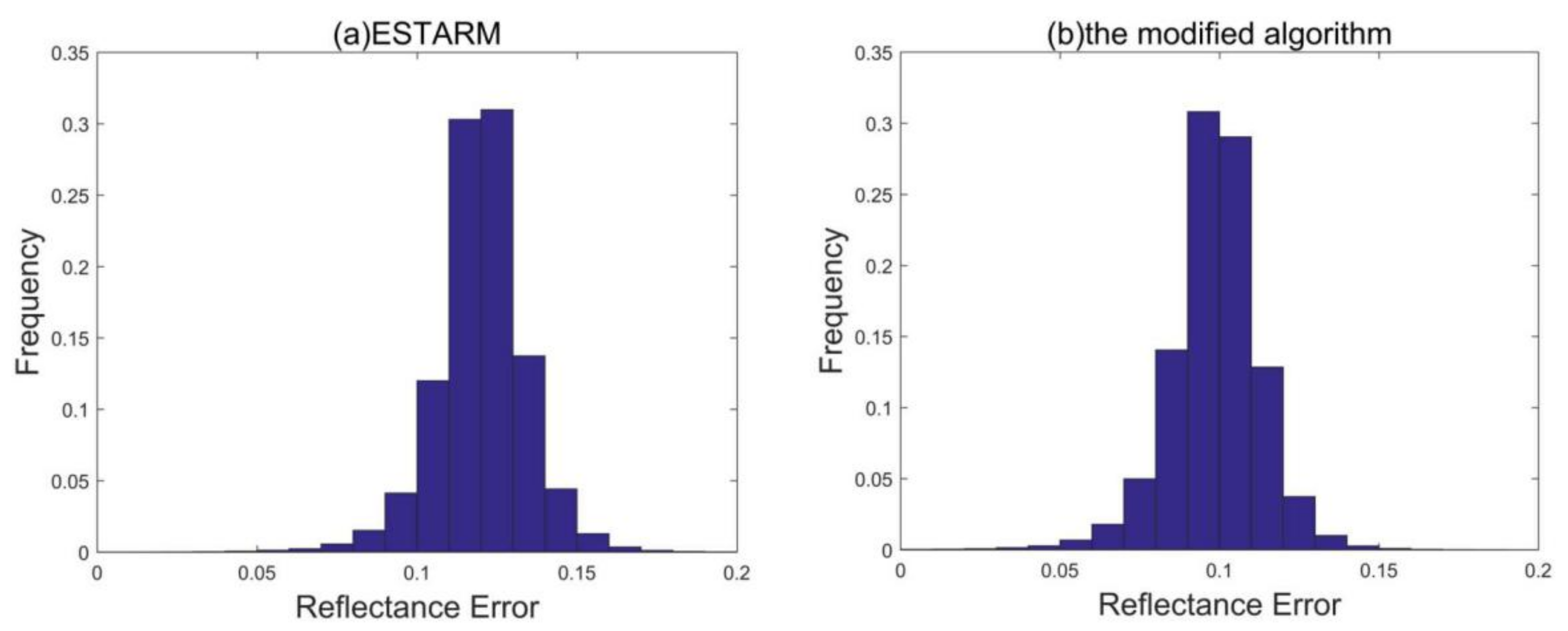
In Figure 6, it is obvious that the spatiotemporal data fusion algorithm using surface heterogeneity information based on ESTARFM performed better than ESTARFM on the whole. The modified algorithm’s accuracy was higher than ESTARFM, especially in the heterogeneous region. At the land cover boundary, such as water and land, the result of modified algorithm was clearer than ESTARFM. In order to objectively evaluate the results’ accuracy, we counted all pixels that took part in the spatiotemporal data fusion and processed them in Figure 7. These results showed that, in the modified algorithm, 85% of pixels had an absolute difference of Rmean between the true observed image and the predicted image between 0 and 0.04 after data standardization, while in ESTARFM, the number was 78%. In general, the spatiotemporal data fusion algorithm’s accuracy using surface heterogeneity information based on ESTARFM was higher than that of ESTARFM.

4.3. Robustness Validation

In order to remove the influence of regions when evaluating the modified algorithm’s prediction accuracy, another remote sensing image from Langfang city, Heibei province, China was selected to verify the robustness of the modified algorithm. In this study, Landsat 8 OLI images on 23 May 2017, 10 July 2017, and 12 September 2017, as well as MODIS eight-day composite reflectance data (MOD09A1) on 17 May 2017, 4 July 2017, and 6 September 2017 were selected to evaluate the accuracy of the results for the two spatiotemporal data fusion algorithms. The size of the verification area was consistent with the size of the study area. In the spatiotemporal data fusion algorithms, the number of land cover types in the two algorithms was 4, which was comprised of buildings, water, crop, and non-crop vegetation. For the moving window size in the ESTARFM algorithm, this study used 50 Landsat pixels [28]. In other words, the moving window size was 1500 m*1500 m. The moving window of the spatiotemporal data fusion algorithm using surface heterogeneity information based on ESTARFM was adaptive and did not need to be set in advance. Finally, we evaluated the prediction accuracy of the predicted image obtained via two spatiotemporal data fusion algorithms. The Rmean of predicted images was selected to compare the accuracy of the two spatiotemporal data fusion algorithms; the results are shown in Figure 8. Moreover, the frequency statistics histogram for the absolute difference of Rmean is shown in Figure 9. Results showed that, in the modified algorithm, 51% of pixels had absolute difference of Rmean between the true observed image and predicted image between 0 and 0.1 after standarization, while it was only 6% in ESTARFM. The spatiotemporal data fusion algorithm using surface heterogeneity information based on ESTARFM had a higher accuracy, as shown in Figure 8 and Figure 9. In addition, the running time of the modified algorithm was less than ESTARFM.

5. Discussion

The modified spatiotemporal data fusion algorithm used mean local variance as the index to measure the spatial heterogeneity of a moving window. Further, the optimal moving window size was selected in the spatiotemporal data fusion algorithm according to the average local variance. The modified algorithm took full advantage of the correlation between the neighborhood pixel and center pixel. The optimal moving window size not only ensured that the appropriate number of similar center pixels participated in the fusion but it also reduced the computation redundancy of the algorithm. Therefore, the spatiotemporal data fusion algorithm efficiency improved. Subjective assessment results showed that the modified algorithm obtained more details than ESTARFM, and objective assessment results showed that the modified algorithm performed better than ESTARFM. Verification test showed the robustness of the modified algorithm. In conclusion, the modified algorithm improved efficiency while still maintaining its prediction accuracy. The flexible moving window strategy provided the basis of the automatic algorithm on a global scale. The modified algorithm provides new idea to spatiotemporal data fusion methods and enriches the spatiotemporal data fusion family. The modified algorithm can be used in heterogeneous regions such as southern China to cover the data shortage in remote sensing time series analysis.
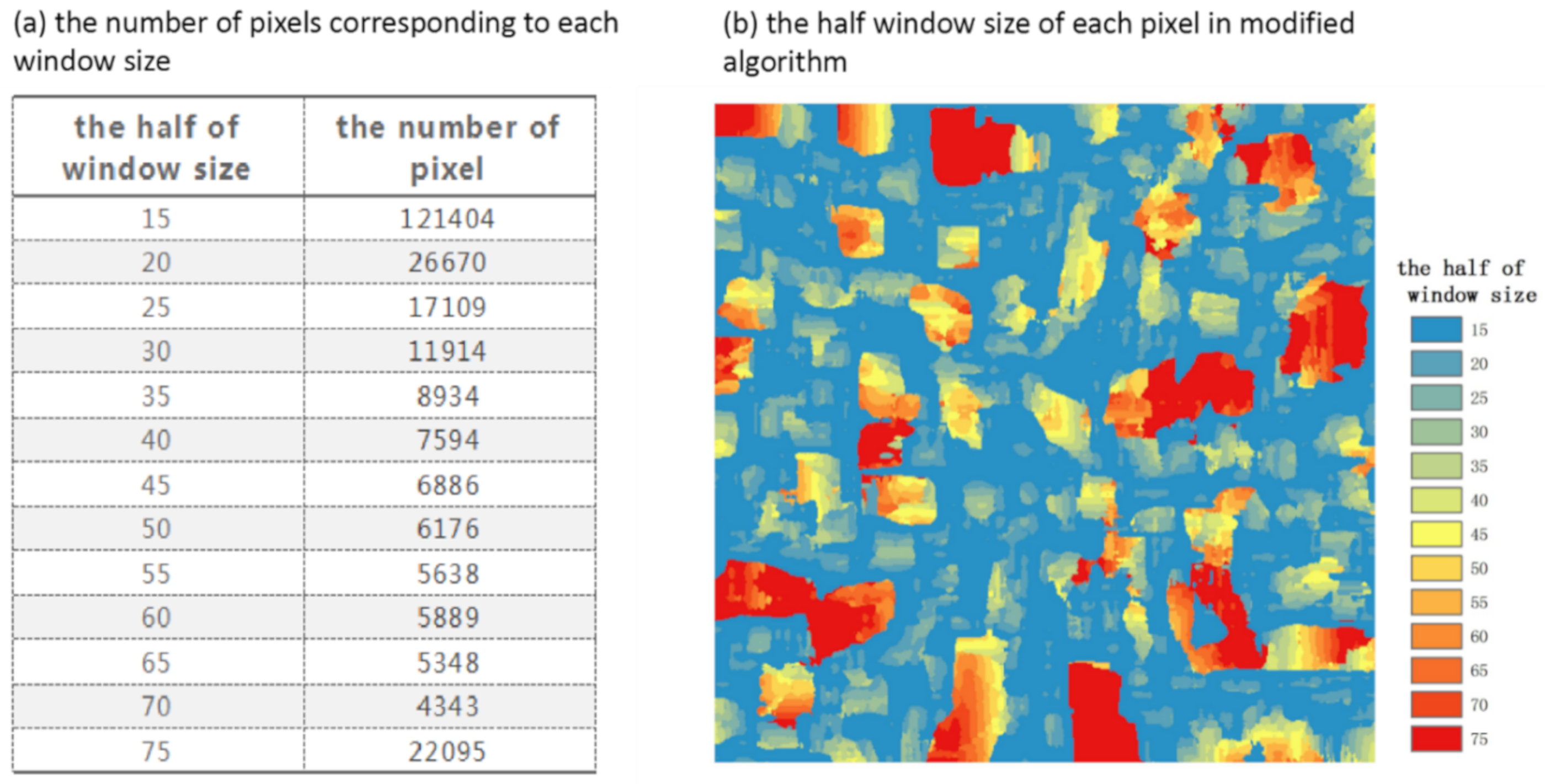
In order to demonstrate the optimal window selected for each pixel in the study sites, we outputted half of the window size in the modified algorithm in Jiujiang and counted the number of pixels that corresponded to each window size. The result is shown in Figure 10 and Figure 11. When comparing the original Landsat image of Jiujiang, it is obvious that the heterogeneous regions became larger in the modified algorithm, while homogeneous regions became smaller. However, this was not the case for the entire study area. The inside reason still requires further study. For the effectiveness of the modified algorithm, we discovered the reason the number of pixels corresponded to each window size. ESTARFM used 25 as the half window size in the modified algorithm, which was 25 of 250,000 pixels for the half window size in ESTARFM. However, 15 of 121,404 pixels (about 48.5%) were used for the half window size in the Jiujiang modified algorithm, which saved a lot of calculation time. Therefore, the modified algorithm efficiency was higher than for ESTARFM in Jiujiang.
Arguably, the spatiotemporal data fusion algorithm that used surface heterogeneity information based on ESTARFM obtained good results in this study to some degree, yet there are still some problems in the research. Firstly, the inconsistency of input image pairs could have affected the fusion results. Although the consistency between Landsat and MODIS data was high, there were some inevitable differences in image angles, acquisition time, geographic registration problem, and data processing methods due to different satellite sensor design. Recent studies have fused Sentinel-2 with Sentinel-3 to generate daily Sentinel-2 images [3], or only fused bands within Sentinel-2 by downscaling bands [42], which partly solved data consistency. However, with the development of unmanned aerial vehicle (UVM) images, it is urgent to fuse UVM images with satellite images in future studies [43]. Hence, it is necessary to develop spatiotemporal data fusion algorithms that can solve the problem of data consistency. Then, the spatial autocorrelation index is often used to measure the spatial correlation degree of natural or social attributes in order to explore the spatial pattern or distribution characteristics of natural or social phenomena. The magnitude of the correlation degree can characterize the spatial pattern and distribution characteristics of the attribute. In this study, average local variance was employed to indicate the surface spatial feature within different sized moving windows, yet other spatial autocorrelation indicators such as local Moran’s I and Getis-Ord Gi* could also have been suitable for adaptive moving windows. Therefore, they deserve to be featured in comparison experiments. Finally, this study was an exploration of the adaptive moving window in the spatiotemporal data fusion algorithm, and the relationship between the surface spatial feature and optimal moving window size needs further study.
Spatiotemporal data fusion algorithms focus on solving the problem of missing data in earth observation. It predicts the reflectance of images according to the time, space, and spectral information of the input images. Although spatiotemporal data fusion methods have been used in many fields, they still have some shortcomings and future development can be improved in the following aspects: accurate calibration of input remote sensing image; capture of land cover changes in fusion; standard methods of precision evaluation of results; and efficiency improvement of algorithms.

6. Conclusions

In order to automatically attain moving window size in a spatiotemporal data fusion algorithm, we introduced surface spatial information in a spatiotemporal data fusion method to improve ESTARFM prediction accuracy and efficiency. A modified spatiotemporal data fusion method using spatial heterogeneity based on ESTARFM was proposed. The modified algorithm concentrated on the contradiction between surface heterogeneity and a fixed-size moving window, and mean local variance was selected to indicate the spatial heterogeneity of the surface. For each center pixel in the modified spatiotemporal data fusion algorithm, the mean local variances in the moving windows with different sizes were calculated, then the moving window of the size corresponding to the maximum mean local variance was selected as the best window to search the similar pixels to the center pixel. To evaluate the accuracy and robustness of the modified algorithm, we used satellite data from two regions. The predicted images of ESTARFM and the modified algorithm were compared with the observed image. The results indicated that the modified algorithm obtained better performance in blue, green, red, and NIR bands than ESTARFM, while accuracy of SWIR1 band remained mostly the same. However, ESTARFM did better in the SWIR2 band than the modified algorithm. Experiments in two regions showed that the running time of the modified algorithm was shorter than ESTARFM. Therefore, this modified algorithm is helpful for vegetation phenology monitoring, change of land cover, and chlorophyll inversion, but it is not suitable in retrieving land surface temperature and mineral discrimination. In general, the results showed that the modified algorithm obtained better performance than ESTARFM in accuracy, efficiency, and robustness. An adaptive moving window strategy in spatiotemporal data fusion method not only enriches the spatiotemporal data fusion methods but provides the possibility for automated processing of spatiotemporal data fusion algorithms at a large scale.

Author Contributions

Conceptualization, M.L. and X.L.; methodology, M.L. and L.W.; software, M.L. and X.Z.; validation, M.L., B.Z. and X.Z.; formal analysis, M.L.; investigation, L.W.; resources, M.L.; data curation, M.L.; writing—original draft preparation, M.L.; writing—review and editing, X.L., L.W. and B.Z.; visualization, M.L., B.Z. and X.Z.; supervision, X.L.; project administration, X.D.; funding acquisition, L.W., H.W. and X.D. All authors have read and agreed to the published version of the manuscript.

Funding

This research was funded by the National Natural Science Foundation of China under Grant 41701387 and 41901259, and the Second Tibetan Plateau Scientific Expedition and Research Program [2019QZKK0608].

Acknowledgments

The Landsat surface reflectance products are available from the United States Geological Survey (https://espa.cr.usgs.gov/index/) and MOD09A1 were obtained from the National Aeronautics and Space Administration (https://ladsweb.modaps.eosdis.nasa.gov/). The authors wish to thank the anonymous reviewers for their constructive comments that helped improve the scholarly quality of the paper.

Conflicts of Interest

The authors declare no conflict of interest.

References

  1. Anoona, N.P.; Katpatal, Y.B. Remote sensing and gis-based analysis to envisage urban sprawl to enhance transport planning in a fast developing indian city. In Applications of Geomatics in Civil Engineering; Springer: Singapore, 2020; pp. 405–412. [Google Scholar]
  2. Li, S. Multisensor remote sensing image fusion using stationary wavelet transform: Effects of basis and decomposition level. Int. J. Wavelets Multiresolut. Inf. Process. 2008, 6, 37–50. [Google Scholar] [CrossRef]
  3. Wang, Q.; Atkinson, P.M. Spatio-temporal fusion for daily sentinel-2 images. Remote Sens. Environ. 2018, 204, 31–42. [Google Scholar] [CrossRef] [Green Version]
  4. Weng, Q.; Fu, P.; Gao, F. Generating daily land surface temperature at landsat resolution by fusing landsat and modis data. Remote Sens. Environ. 2014, 145, 55–67. [Google Scholar] [CrossRef]
  5. Zou, X.; Liu, X.; Liu, M.; Liu, M.; Zhang, B. A framework for rice heavy metal stress monitoring based on phenological phase space and temporal profile analysis. Int. J. Environ. Res. Public Health 2019, 16, 350. [Google Scholar] [CrossRef] [Green Version]
  6. Zhang, B.; Liu, X.; Liu, M.; Meng, Y. Detection of rice phenological variations under heavy metal stress by means of blended landsat and modis image time series. Remote Sens. 2019, 11, 13. [Google Scholar] [CrossRef] [Green Version]
  7. Lu, Y.; Wu, P.; Ma, X.; Li, X. Detection and prediction of land use/land cover change using spatiotemporal data fusion and the cellular automata–markov model. Environ. Monit. Assess. 2019, 191, 68. [Google Scholar] [CrossRef] [PubMed]
  8. Wu, P.; Shen, H.; Zhang, L.; Göttsche, F.-M. Integrated fusion of multi-scale polar-orbiting and geostationary satellite observations for the mapping of high spatial and temporal resolution land surface temperature. Remote Sens. Environ. 2015, 156, 169–181. [Google Scholar] [CrossRef]
  9. Zhu, X.; Cai, F.; Tian, J.; Williams, K.A. Spatiotemporal fusion of multisource remote sensing data: Literature survey, taxonomy, principles, applications, and future directions. Remote Sens. 2018, 10, 527. [Google Scholar]
  10. Niu, Z.; Wu, M.; Wang, C. Use of modis and landsat time series data to generate high-resolution temporal synthetic landsat data using a spatial and temporal reflectance fusion model. J. Appl. Remote Sens. 2012, 6, 63507. [Google Scholar] [CrossRef]
  11. Zurita-Milla, R.; Clevers, J.G.P.W.; Schdepman, M.E. Unmixing-based landsat tm and meris fr data fusion. IEEE Geosci. Remote Sens. Lett. 2008, 5, 453–457. [Google Scholar] [CrossRef] [Green Version]
  12. Zhang, W.; Li, A.; Jin, H.; Bian, J.; Zhang, Z.; Lei, G.; Qin, Z.; Huang, C. An enhanced spatial and temporal data fusion model for fusing landsat and modis surface reflectance to generate high temporal landsat-like data. Remote Sens. 2013, 5, 5346–5368. [Google Scholar] [CrossRef] [Green Version]
  13. Dongjie, F.; Baozhang, C.; Juan, W.; Xiaolin, Z.; Thomas, H. An improved image fusion approach based on enhanced spatial and temporal the adaptive reflectance fusion model. Remote Sens. 2013, 5, 6346–6360. [Google Scholar]
  14. Wu, B.; Huang, B.; Cao, K.; Zhuo, G. Improving spatiotemporal reflectance fusion using image inpainting and steering kernel regression techniques. Int. J. Remote Sens. 2016, 38, 706–727. [Google Scholar] [CrossRef]
  15. Jie, X.; Yee, L.; Tung, F. A bayesian data fusion approach to spatio-temporal fusion of remotely sensed images. Remote Sens. 2017, 9, 1310. [Google Scholar]
  16. Shen, H.; Meng, X.; Zhang, L. An integrated framework for the spatio–temporal–spectral fusion of remote sensing images. IEEE Trans. Geosci. Remote Sens. 2016, 54, 7135–7148. [Google Scholar] [CrossRef]
  17. Huang, B.; Zhang, H.; Song, H.; Wang, J.; Song, C. Unified fusion of remote-sensing imagery: Generating simultaneously high-resolution synthetic spatial–temporal–spectral earth observations. Remote Sens. Lett. 2013, 4, 561–569. [Google Scholar] [CrossRef]
  18. Huang, B.; Song, H. Spatiotemporal reflectance fusion via sparse representation. IEEE Trans. Geosci. Remote Sens. 2012, 50, 3707–3716. [Google Scholar] [CrossRef]
  19. Wu, B.; Huang, B.; Zhang, L. An error-bound-regularized sparse coding for spatiotemporal reflectance fusion. IEEE Trans. Geosci. Remote Sens. 2015, 53, 6791–6803. [Google Scholar] [CrossRef]
  20. Song, H.; Liu, Q.; Wang, G.; Hang, R.; Huang, B. Spatiotemporal satellite image fusion using deep convolutional neural networks. IEEE J. Sel. Top. Appl. Earth Obs. Remote Sens. 2018, 11, 821–829. [Google Scholar] [CrossRef]
  21. Gevaert, C.M.; García-Haro, F.J. A comparison of starfm and an unmixing-based algorithm for landsat and modis data fusion. Remote Sens. Environ. 2015, 156, 34–44. [Google Scholar] [CrossRef]
  22. Li, X.; Ling, F.; Foody, G.M.; Ge, Y.; Zhang, Y.; Du, Y. Generating a series of fine spatial and temporal resolution land cover maps by fusing coarse spatial resolution remotely sensed images and fine spatial resolution land cover maps. Remote Sens. Environ. 2017, 196, 293–311. [Google Scholar] [CrossRef]
  23. Rao, Y.; Xiaolin, Z.; Jin, C.; Jianmin, W. An improved method for producing high spatial-resolution ndvi time series datasets with multi-temporal modis ndvi data and landsat tm/etm+ images. Remote Sens. 2015, 7, 7865–7891. [Google Scholar] [CrossRef] [Green Version]
  24. Gao, F.; Masek, J.; Schwaller, M.; Hall, F. On the blending of the landsat and modis surface reflectance: Predicting daily landsat surface reflectance. IEEE Trans. Geosci. Remote Sens. 2006, 44, 2207–2218. [Google Scholar]
  25. Walker, J.J.; Beurs, K.M.D.; Wynne, R.H.; Gao, F. Evaluation of landsat and modis data fusion products for analysis of dryland forest phenology. Remote Sens. Environ. 2012, 117, 381–393. [Google Scholar] [CrossRef]
  26. Olsoy, P.J.; Mitchell, J.; Glenn, N.F.; Flores, A.N. Assessing a multi-platform data fusion technique in capturing spatiotemporal dynamics of heterogeneous dryland ecosystems in topographically complex terrain. Remote Sens. 2017, 9, 981. [Google Scholar] [CrossRef] [Green Version]
  27. Hilker, T.; Wulder, M.A.; Coops, N.C.; Seitz, N.; White, J.C.; Gao, F.; Masek, J.G.; Stenhouse, G. Generation of dense time series synthetic landsat data through data blending with modis using a spatial and temporal adaptive reflectance fusion model. Remote Sens. Environ. 2009, 113, 1988–1999. [Google Scholar] [CrossRef]
  28. Zhu, X.; Chen, J.; Gao, F.; Chen, X.; Masek, J.G. An enhanced spatial and temporal adaptive reflectance fusion model for complex heterogeneous regions. Remote Sens. Environ. 2010, 114, 2610–2623. [Google Scholar] [CrossRef]
  29. Wang, P.; Gao, F.; Masek, J.G. Operational data fusion framework for building frequent landsat-like imagery. IEEE Trans. Geosci. Remote Sens. 2014, 52, 7353–7365. [Google Scholar] [CrossRef]
  30. Moosavi, V.; Talebi, A.; Mokhtari, M.H.; Shamsi, S.R.F.; Niazi, Y. A wavelet-artificial intelligence fusion approach (waifa) for blending landsat and modis surface temperature. Remote Sens. Environ. 2015, 169, 243–254. [Google Scholar] [CrossRef]
  31. Liu, X.; Deng, C.; Chanussot, J.; Hong, D.; Zhao, B. Stfnet: A two-stream convolutional neural network for spatiotemporal image fusion. IEEE Trans. Geosci. Remote Sens. 2019, 57, 6552–6564. [Google Scholar] [CrossRef]
  32. Gao, F.; Hilker, T.; Zhu, X.; Anderson, M.; Masek, J.; Wang, P.; Yang, Y. Fusing landsat and modis data for vegetation monitoring. IEEE Geosci. Remote Sens. Mag. 2015, 3, 47–60. [Google Scholar] [CrossRef]
  33. Chen, Y.; Jian-Ping, W.U. Spatial autocorrelation analysis on local economy of three economic regions in eastern china. Sci. Surv. Mapp. 2013, 38, 89–92. [Google Scholar]
  34. Markham, B.L.; Storey, J.C.; Williams, D.L.; Irons, J.R. Landsat sensor performance: History and current status. IEEE Trans. Geosci. Remote Sens. 2004, 42, 2691–2694. [Google Scholar] [CrossRef]
  35. Carlson, T.N.; Arthur, S.T. The impact of land use—Land cover changes due to urbanization on surface microclimate and hydrology: A satellite perspective. Glob. Planet. Chang. 2000, 25, 49–65. [Google Scholar] [CrossRef]
  36. Ryu, J.H.; Won, J.-S.; Min, K.D. Waterline extraction from landsat tm data in a tidal flat: A case study in gomso bay, korea. Remote Sens. Environ. 2002, 83, 442–456. [Google Scholar] [CrossRef]
  37. Miller, H.J. Tobler’s first law and spatial analysis. Ann. Assoc. Am. Geogr. 2004, 94, 284–289. [Google Scholar] [CrossRef]
  38. Tobler, W.R. A computer movie simulating urban growth in the detroit region. Econ. Geogr. 1970, 46, 234. [Google Scholar] [CrossRef]
  39. Liu, M.; Liu, X.; Wu, L.; Zou, X.; Jiang, T.; Zhao, B. A modified spatiotemporal fusion algorithm using phenological information for predicting reflectance of paddy rice in southern china. Remote Sens. 2018, 10, 772. [Google Scholar] [CrossRef] [Green Version]
  40. Li, S.; Li, Z.; Gong, J. Multivariate statistical analysis of measures for assessing the quality of image fusion. Int. J. Image Data Fusion 2010, 1, 47–66. [Google Scholar] [CrossRef]
  41. Wang, Z.J.; Ziou, D.; Armenakis, C.; Li, D.R.; Li, Q.Q. A comparative analysis of image fusion methods. IEEE Trans. Geosci. Remote Sens. 2005, 43, 1391–1402. [Google Scholar] [CrossRef]
  42. Wang, Q.; Shi, W.; Li, Z.; Atkinson, P.M. Fusion of sentinel-2 images. Remote Sens. Environ. 2016, 187, 241–252. [Google Scholar] [CrossRef] [Green Version]
  43. Kakooei, M.; Baleghi, Y. Fusion of satellite, aircraft, and uav data for automatic disaster damage assessment. Int. J. Remote. Sens. 2017, 38, 2511–2534. [Google Scholar] [CrossRef]
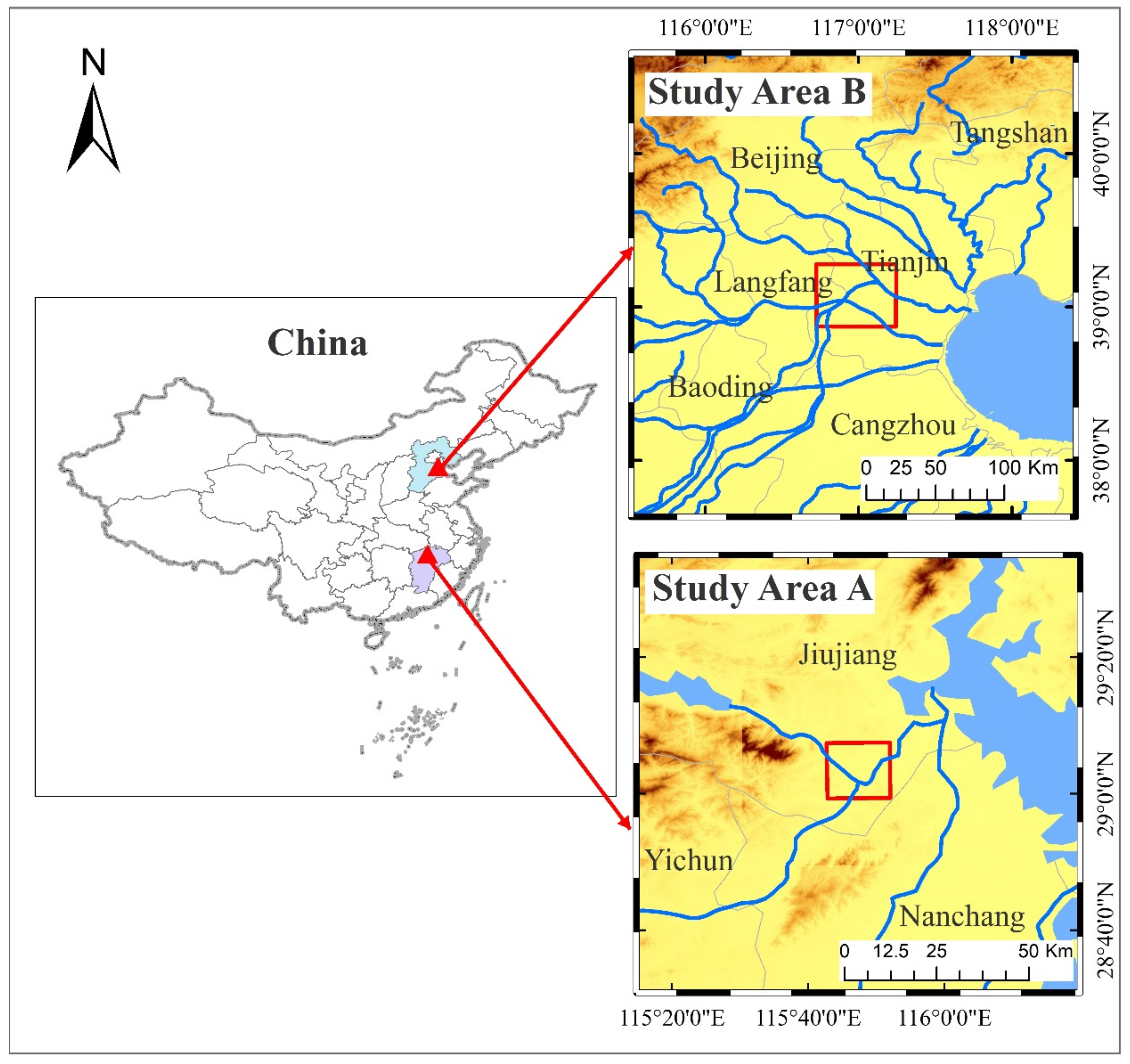
Figure 1. Location map of study areas. Study area A is located in Jiujiang, Jiangxi Province, while study area B is located in Langfang, Hebei Province.
Remotesensing 12 03673 g001
Figure 2. The schematic diagram of the adaptive moving window strategy in the spatiotemporal data fusion method.
Remotesensing 12 03673 g002
Figure 3. The algorithm flow of an adaptive moving window strategy in the spatiotemporal data fusion method.
Remotesensing 12 03673 g003
Figure 4. The comparison of actual images and predicted images using different spatiotemporal data fusion algorithms. Note: the upper row are true-color-composites of Landsat and Landsat-like images; the lower row are false-color-composites of Landsat and Landsat-like images; (a,d) are actual observed images; (b,e) are Landsat-like images predicted by ESTARFM; (c,f) are Landsat-like images predicted by the modified algorithm.
Remotesensing 12 03673 g004
Figure 5. The comparison of actual images and predicted images using different spatiotemporal data fusion algorithms. (a) is the actual image; (b) is the predicted image by ESTARFM; (c) is the predicted images by the modified algorithm.
Remotesensing 12 03673 g005
Figure 6. Scatter plots of the actual reflectance values and estimated values by the ESTARFM (left column, a,c,e,g,i,k) and modified algorithm (right column, b,d,f,h,j,l).
Remotesensing 12 03673 g006
Figure 7. The comparison of the absolute difference of Rmean between the true observed image and predicted image by ESTARFM (a) and the modified algorithm (b).
Remotesensing 12 03673 g007
Figure 8. Frequency statistics histogram of the Rmean absolute difference of results predicted by ESTARFM (a) and the modified algorithm (b) in Jiujiang.
Remotesensing 12 03673 g008
Figure 9. The comparison of the absolute difference of Rmeanbetween the true observed image and the predicted image by ESTARFM (a) and the modified algorithm (b) in Langfang.
Remotesensing 12 03673 g009
Figure 10. Frequency statistics histogram of the Rmean absolute difference of results predicted by ESTARFM (a) and the modified algorithm (b) in results of Langfang.
Remotesensing 12 03673 g010
Figure 11. The use of different window sizes in the algorithm in Jiujiang. (a) is statistical table of number of pixels corresponding to each window size and (b) is the distribution map of the half window size of each pixel in the modified algorithm.
Remotesensing 12 03673 g011
Table 1. Information of corresponding bands of Landsat7 ETM+, Landsat8 OLI, and MODIS.
BandLandsat7 ETM+Bandwidth (nm)Landsat8 OLIBandwidth (nm) MODISBandwidth (nm)
BlueBand 1450–520Band 2450–510Band 3459–479
GreenBand 2530–610Band 3530–590Band 4545–565
RedBand 3450–510Band 4630–690Band 1620–670
Near Infrared (NIR)Band 4780–900Band 5850–880Band 2841–876
Short-Wave Infrared 1 (SWIR1)Band 51550–1750Band 61570–1650Band 61628–1652
Short-Wave Infrared 2 (SWIR2)Band 62090–2350Band 72110–2290Band 72105–2155
Table 2. Remote sensing data types and acquisition date.
RegionData TypeSpatial ResolutionPath/RowAcquisition DateUse
Study Area A(Jiujiang)Landsat7 ETM+30 m122/402013/7/24Image fusion
122/392013/8/9Accuracy assessment
122/402013/9/10Image fusion
MOD09A1500 mh27v062013/7/20Image fusion
2013/8/5Image fusion
2013/9/6Image fusion
Study Area B(Langfang)Landsat8 OLI30 m 2017/5/23Image fusion
123/322017/7/10Accuracy assessment
2017/9/12Image fusion
MOD09A1500 mh26v042017/5/17Image fusion
2017/7/4Image fusion
2017/9/6Image fusion
Table 3. Quantitative comparison of the prediction accuracy of ESTARFM and the modified algorithm.
Reflectance ESTARFMThe Modified Algorithm
Land CoverBandρrRSMEρrRMSE
BuildingBand 10.8046 0.7888 168.5 0.8134 0.7926 167.2
Band 20.9127 0.8116 173.2 0.9424 0.8198 168.7
Band 30.9648 0.8629 288.1 1.0174 0.8760 281.9
Band 40.7791 0.7967 370.5 0.8184 0.8095 352.5
Band 50.8003 0.7945 421.0 0.8495 0.7974 409.1
Band 60.9665 0.8627389.2 0.9801 0.8598 388.6
WaterBand 10.4702 0.6616 199.9 0.5243 0.6845 179.4
Band 20.5847 0.7350 247.6 0.6736 0.7649 215.8
Band 30.4893 0.6868 281.7 0.5737 0.7285 241.1
Band 40.4060 0.5640 527.7 0.4282 0.5867 520.2
Band 50.1879 0.3362 548.5 0.2070 0.3607 541.9
Band 60.21320.3727251.40.2039 0.3674 259.2
PaddyBand 10.5554 0.6530 86.8 0.6335 0.7092 78.2
Band 20.7055 0.6651 113.6 0.7727 0.7084 105.8
Band 30.7774 0.7306 120.4 0.8718 0.7863 105.2
Band 40.5167 0.5206 420.80.5442 0.5349 426.8
Band 50.6592 0.6865 405.2 0.7154 0.7168 394.4
Band 60.80720.7448177.10.8036 0.7434 177.3
Non-paddy vegetationBand 10.5211 0.6048 98.6 0.6088 0.6511 88.1
Band 20.5443 0.6616 128.5 0.6097 0.6917 125.0
Band 30.6514 0.6739 138.0 0.7646 0.7339 121.5
Band 40.5833 0.6848 359.7 0.6620 0.7286 316.6
Band 50.6419 0.7631 378.2 0.6680 0.7827 359.8
Band 60.7698 0.7703 180.0 0.7872 0.7826 174.0
Note: The better results of ESTARFM are highlighted in bold.
Publisher’s Note: MDPI stays neutral with regard to jurisdictional claims in published maps and institutional affiliations.