Abstract
Capturing high spatial resolution imagery is becoming a standard operation in many agricultural applications. The increased capacity for image capture necessitates corresponding advances in analysis algorithms. This study introduces automated raster geoprocessing methods to automatically extract strawberry (Fragaria × ananassa) canopy size metrics using raster image analysis and utilize the extracted metrics in statistical modeling of strawberry dry weight. Automated canopy delineation and canopy size metrics extraction models were developed and implemented using ArcMap software v 10.7 and made available by the authors. The workflows were demonstrated using high spatial resolution (1 mm resolution) orthoimages and digital surface models (2 mm) of 34 strawberry plots (each containing 17 different plant genotypes) planted on raised beds. The images were captured on a weekly basis throughout the strawberry growing season (16 weeks) between early November and late February. The results of extracting four canopy size metrics (area, volume, average height, and height standard deviation) using automatically delineated and visually interpreted canopies were compared. The trends observed in the differences between canopy metrics extracted using the automatically delineated and visually interpreted canopies showed no significant differences. The R2 values of the models were 0.77 and 0.76 for the two datasets and the leave-one-out (LOO) cross validation root mean square error (RMSE) of the two models were 9.2 g and 9.4 g, respectively. The results show the feasibility of using automated methods for canopy delineation and canopy metric extraction to support plant phenotyping applications.
1. Introduction
The use of high-resolution remote sensing technologies established deep roots in the natural resource and agricultural management fields [1,2]. Through the ability to collect high spatial, temporal and spectral resolution data, remote sensing provides a plethora of information supporting a broad spectrum of applications. For example, remotely sensed imagery provides timely information to assist operations involving nutrient concentration modeling, disease detection, and water stress assessment [3,4,5,6]. Information derived from remote sensing imagery has benefitted growth monitoring and yield modeling [7,8,9]. Breeding programs benefit from diverse, low cost, and high throughput remote sensing technologies capable of measuring plant traits [10,11,12].
Interactive analysis of remote sensing data can be beneficial for data exploration; however, the current flood of remote sensing datasets mandates the development of automated analysis methods that are efficient, adaptable, and easy to use. This is especially important to reduce the cost and increase the benefit of using these technologies and to efficiently apply them to small farms and research experiments that are typical for specialty crops such as strawberries. Many remote sensing applications focus on utilizing the spectral information in the images using spectral indices, for example, with less emphasis on geometrical canopy characteristics that can also be extracted from the images. Spectral differences in the images due to the interaction of electromagnetic radiation with the plants and their surroundings enable many of the applications, especially if the images are capable of sensing energies from multiple areas of the electromagnetic spectrum and in narrow spectral bands [13,14,15]. Spectral information has been used to infer vegetation biophysical parameters such as leaf area and biomass, which are related to canopy sizes and structure, and are necessary for ecological and climate change models [16].
Geometric properties of scene objects such as canopy height and volume require higher geospatial accuracy, higher spatial resolution, and specific analysis tools for data extraction [17,18,19]. Explicit modeling of canopy size and structure is facilitated using lidar datasets, where 3D points of the canopy and ground are retrieved when the laser photons infiltrate within canopy, hit different under-canopy strata, and reflect back to the sensor, providing coordinates of all return points [20]. Wu et al. [21] utilized a high-density lidar system mounted on an unpiloted aircraft vehicle (UAV-lidar) to detect individual tree canopies and estimate canopy cover. The authors tested watershed segmentation, polynomial fitting, individual tree crown segmentation (ITCS), and point cloud segmentation (PCS) algorithms. The results showed the PCS and ITCS algorithms produced the best canopy segmentation results. Lidar data acquisition, however, is still very expensive to implement and integrate in farm operations, which typically require frequent data collection throughout the growing season [21].
Several tree detection and canopy delineation algorithms from high resolution imagery were reviewed in Ke and Quakenbush [22]. Early efforts for canopy delineation focused mainly on using orthorectified imagery (orthoimages). For example, Jiang et al. [23] developed a canopy delineation algorithm based on multiscale segmentation and watershed segmentation of orthorectified imagery produced using aerial images. Typically, high-resolution aerial imagery is analyzed using photogrammetric techniques to produce 3D point clouds in addition to the orthoimages. Image-derived 3D point clouds have been used recently for canopy delineation; however, these points only represent the visible top layer of the canopy and hence they do not provide information about interior canopy structure and under-canopy ground elevations. Marasigan et al. [24] demonstrated the use of the marker-controlled watershed algorithm (MCWA) [25,26] to delineate individual canopies using canopy heights as the difference between canopy top and ground elevations. Huang et al. [27] applied the bias field estimation used in medical image segmentation and MCWA to identify individual tree canopies from unpiloted aircraft systems (UASs) imagery with 2.5 cm resolution. The authors used local intensity smoothing before clustering as a preprocessing step. These studies have not particularly addressed the extraction of canopy size metrics. Points returned from the ground under the canopy are necessary for canopy metric estimation and are not available for image-based datasets. This requires the development of other algorithms to model ground elevations, especially when complex ground structures such as raised beds are utilized.
Some studies have recently attempted to model agricultural crop biophysical parameters such as biomass using high resolution imagery, with spectral and spatial information [28,29]. Maimaitijiang et al. [30] used vegetation spectral, volumetric, and structural indices to estimate soybeans biomass. Extracting barley height in an effort to model biomass from high resolution imagery captured by unmanned aircraft systems (UASs) was conducted by Bendig et al. [31] and Brocks et al. [32]. Most of this research involves vegetation types that do not have a bush growth pattern and do not grow on raised beds like strawberries, which significantly complicates canopy size metric extraction. Several algorithms to delineate canopies and extract vegetation structure metrics from lidar data have been developed [21,22,23]. Guan et al. [19] utilized an object-based analysis to extract canopy metrics. Interactive step-by-step implementation and software and computational cost associated with using an object-based analysis highlight the need to develop automated raster-based geoprocessing workflow for canopy size metric extraction.
This study introduces geospatial analysis workflows for automated extraction of strawberry canopy geometric information as a typical example of a small, herbaceous crop with a bushy growth habit planted on raised beds. The study introduces an end-to-end raster-based geospatial analysis workflow applied on ultra-high spatial resolution images (0.5-mm per pixel for raw images) and dense point clouds (more than 100,000 pts/m2) to extract canopy metrics (area, volume, average height, and height standard deviation). The canopy delineation and size metric extraction models developed in this manuscript introduce several techniques to analyze not only strawberry canopies, but also other crops with different canopy and field configurations. For example, the manuscript utilized directional interpolation to fill the gaps in bed elevations under the canopies, which is a major limitation in photogrammetry derived elevation models compared to lidar products, which are capable of getting under-canopy ground returns. The same applies to identifying soil elevations using mesh analysis and utilizing these elevations for weed filtering. The extracted canopy metrics were tested on a phenomics experiment conducted throughout the 2017/2018 strawberry growing season to model dry biomass of 17 strawberry genotypes. The results of implementing the developed canopy delineation workflow were compared to the canopies delineated using visual interpretation of canopy boundaries. Different cross validation methods were also used to assess results.
2. Study Site and Data Preparation
2.1. Study Site
The University of Florida’s Gulf Coast Research and Education Center (GCREC) experimental farm in Wimauma, FL, 27°45′40″N and 82°13′40″W (Figure 1) housed the study site for this research. Strawberries were planted according to commercial standards on two adjacent one-hundred-meter long raised beds. Each of the two beds contained 17 plots and each plot contained 17 plants, one of each of 17 strawberry genotypes (Table 1) used in this experiment, for a total of 34 plots. The range of canopy structures for the 17 selected genotypes was representative of the University of Florida’s strawberry breeding germplasm. Approximately once a week, between 16th November and 27th February, images were collected for a total of 16 sets of images throughout the Florida winter strawberry growing season. The images were collected for six adjacent beds, the two study beds and two additional beds on each side (Figure 1), allowing for strong photogrammetric geometry for image analysis. Figure 1 also shows the layout of one plot as designed and implemented.
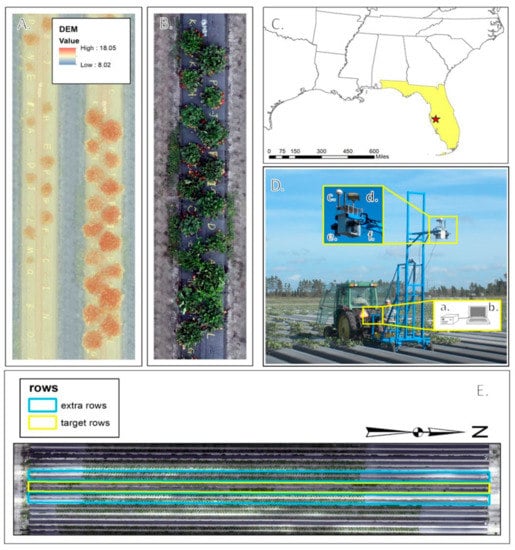
Figure 1.
Experimental location, setup, and equipment. (A). Digital Surface Model viewed over orthoimage of a plot. (B). Individual plot layout showing plant genotype alphabetical codes. (C). Location of Gulf Coast Research and Education Center in Wimauma, FL, the site of this experiment. (D). Imaging platform equipped with a. synchronization and acquisition software (laptop), a,b. camera trigger box hardware, c. timing GPS, d. survey-quality GNSS receiver, e. Nikon D300 RGB camera, and f. Nikon D300 IR camera. (E). Six rows of data collection centering over two target rows.

Table 1.
Statistical summary of dry biomass in grams of 17 genotypes (left) and 16 acquisition dates (right).
2.2. Image Data Acquisition and Preprocessing
The images used in this study were acquired using the set-up introduced by Abd-Elrahman et al. [33,34] to collect ground-based images from a platform towed by a tractor in a strawberry field (Figure 1). Two Nikon D300 cameras were used. One of the cameras captured RGB images while the other camera was modified to capture IR images. The cameras were mounted 20 cm apart on the platform and triggered simultaneously every two seconds. Each image was tagged with a Trimble Accutime Gold Global Positioning System (GPS) timestamp using custom-built synchronization hardware. Each image exposure location was determined in post-acquisition analysis by interpolating the image location from the trajectory obtained by a Topcon Hiper Lite plus survey-grade Global Navigation Satellite System (GNSS) receiver onboard the platform. The images were acquired approximately 3.5 m above the ground with the platform moving at 0.5 m/sec providing 70% image overlap and 60% sidelap. This configuration allows for photogrammetric analysis of the images to produce point clouds, orthoimages, and Digital Surface Model (DSM) [35,36]. The four beds adjacent to those containing the plots (two from each side) were also surveyed to provide overlapping images for the photogrammetric analysis as shown in Figure 1.
Centimeter-level accuracy ground control points were established in the study area as described by Guan et al. [19] using a survey-grade total station and static GNSS observations. The control points were established to be visible in the images and used in the structure from motion (SfM) photogrammetric solution to produce orthoimages and DSM [37]. The SfM technique is used widely to process overlapping images captured by multiple platforms (e.g., UAS and piloted aircrafts) in the agriculture and natural resource management fields.
SfM is a workflow combining photogrammetric and computer vision techniques to generate 3D products from 2D images. The first task within SfM is to match overlapped images taken from different angles and locations to identify common features. The locations of these matched features are used to accurately estimate camera and scene geometry at the time of each image exposure [38]. Specifically, the matched image features, along with surveyed ground control points, are used as input into a bundle-block adjustment process [39] that is solved mathematically to estimate the position and angular orientation of each camera at the moment of exposure. This process is followed by another, denser image matching process to identify conjugate image locations covering the entire scene that can be used, with the image exterior orientation parameters, to produce a dense 3D point cloud representing the features in the scene. The same dataset can also be used to create an orthorectified image mosaic that is free from perspective distortions related to tilt of the camera and feature relief. This type of analysis enables post processing of the orthoimage, 3D point clouds, and conducting multi-view analysis [40].
In this study, the SfM Agisoft Photoscan software (version 1.4.0.5650) [41] was used to produce 1 mm ground sample distance (GSD) RGB/IR orthoimages and 2 mm DSM standard products. The orthoimage products were corrected for the effects of camera tilt and scene topography variations, and were used to acquire planimetric measurements.
2.3. Information Derived from the Orthoimages
Spectral indices such as the normalized difference vegetation index (NDVI) [42], shadow ratio [43,44], and the saturation value of the hue–intensity–saturation color model [45] were produced as raster layers. Pixels with saturation greater than 0.4, NDVI greater than 0, and shadow ratio less than 0 were classified as vegetation. The thresholds for the saturation and NDVI were determined by testing multiple thresholds and visually assessing the results, while the shadow ratio threshold was determined by previous research results [43,44]. All thresholds were held constant and applied to all the datasets acquired throughout the season. The vegetation class was used as a mask to differentiate between vegetated and non-vegetated (soils and bed) areas in the canopy delineation and size metrics extraction workflows introduced in the subsequent sections.
2.4. In-Situ Dry Biomass Measurements
Dry biomass samples were collected from each plant using destructive sampling within several hours of image acquisition. Each week, two plots, one from each bed, were randomly selected and the plants from these plots were taken to the laboratory to measure dry biomass following image acquisition. For each canopy, the leaves were bagged and then placed in a drying oven at 65 °C for five days. The dry biomass [46] weight was then measured. The dry biomass was used as the dependent variable in the regression analysis utilizing image-derived canopy size metrics as independent variables. Table 1 shows statistical summaries of the dry biomass measured in this experiment organized by strawberry genotypes and acquisition dates.
3. Methodology
3.1. Canopy Delineation Workflow
Individual strawberry canopy boundaries were used to extract canopy size metrics. A geospatial analysis workflow was developed to delineate individual plant boundaries. The workflow involves preparing the images and utilized the marker-controlled watershed algorithm implemented in the ‘mcws’ function of the ForestTools R package [47]. The function uses a vector layer containing a point for each plant canopy located at the highest point of the canopy and a raster layer representing canopy heights. The raster layer output from the watershed delineation process is post-processed to create a vector polygon layer representing each canopy boundary. This workflow was implemented using four different models developed using ESRI’s ArcMap v10.7 [48] Model Builder, where various geoprocessing functions including those belonging to the Spatial Analyst extension of the software were used.
The workflow was divided into four different subsequent models to allow inspection and analysis of the results of each model (or step). The input datasets of the whole workflow were three basic datasets: (1) vegetation mask produced as explained in Section 2.3, (2) DSM produced using the SfM algorithm, and (3) a layer containing a single point approximately located at the center of each plant. Since canopy points did not need to be positioned accurately at the center of the plant, a single point layer was produced and used for all the datasets acquired throughout the strawberry season (16 datasets). An optional layer outlining the boundary of the field site was used to clip the datasets to a tighter field boundary, which led to a smaller analysis extent, and hence shorter processing time. The developed four-part (four-models) workflow is described below and illustrated in Figure 2 and Figure 3A. The developed models and associated code are available for researchers through direct request to this article’s corresponding author.
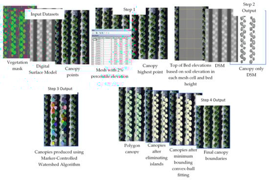
Figure 2.
Illustration of the automated canopy delineation processes.
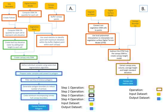
Figure 3.
A. Automated canopy boundary delineation workflow and B. Canopy size metrics extraction workflow.
- Model 1: The highest point within each canopy was determined using approximate locations. A single approximate location representing each canopy was used to automatically find the highest point of the canopy using the DSM. These points were needed for the watershed algorithm to delineate the canopy. The study area was divided into 1 m square cells (fishnet) and the 2% elevation quantile of the DSM within each cell was extracted. The 2% quantile was the DSM elevation value where 98% of the pixels within each cell were higher. This elevation was chosen to represent the soil (between beds) elevations within each cell in the field. A 1 m grid was used for the strawberry field, which guaranteed that soils represented at least 2% of each cell. A python script customized by the authors based on the ArcGIS user community (https://community.esri.com/thread/95403#555075) was used to compute the quantiles. The script was embedded as a tool within model 1 in ArcMap.
- Model 2: Vegetation pixels lower than bed elevation, which is the 2% quantile elevation in each cell plus bed height (15 cm in this field) were filtered out. These pixels were excluded from the analysis since they either represented weeds growing from the soil or canopy leaves extending outside the bed boundary. In both cases, our experiments showed that excluding the vegetation areas that satisfied this criteria improved analysis results.
- Model 3: The watershed algorithm for canopy delineation was implemented [25,26]. The algorithm used a DSM model restricted to the vegetation mask areas and the highest point inside each canopy to delineate canopy boundary and output the results as a raster layer.
- Model 4: A series of operations were used to convert the raster output of the watershed algorithm to a vector layer, generalize the polygons representing canopy boundaries, eliminate island polygons, and implement a minimum bounding convex hull algorithm to improve the shape of the canopy to complete post-delineation canopy enhancement.
3.2. Canopy Size Metrics Extraction
Individual plant canopy area, volume, average height, and standard deviation of height were computed using a model that iterated through all datasets acquired throughout the season. The Spatial Analyst extension of the ArcMap software v10.7 was used to analyze the raster datasets. A key component of the workflow was to compute strawberry canopy height models as the difference between two elevation surfaces. The first surface was the DSM produced by the SfM solution, which represents the elevation of the top of the objects in the images (top of canopy surface, exposed beds, and soils). The second surface was the digital terrain model (DTM), which represents the elevations after removing the canopies. The latter surface could not be produced directly from the images due to the existence of the vegetation cover. To solve this issue and create the vegetation-free DTM, the local polynomial interpolation technique with a strong directional emphasis in the along-bed direction was used to interpolate the DTM using the elevations of the areas with no vegetation coverage as shown in Figure 4.
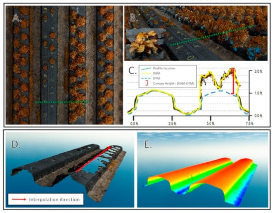
Figure 4.
Point cloud analysis. (A). Planimetric view of point cloud with profile location. (B). Oblique view of profile with inset high resolution view of an individual plant canopy. (C). Profile view of location with DSM, digital terrain model (DTM), and canopy height calculation shown. (D). View of bed with vegetation points removed. (E). Interpolated DTM using along bed directional emphasis.
The difference between the DSM and the DTM provided the canopy height models, which were used in combination with the individual canopy boundaries to compute canopy size metrics. The workflow developed to extract canopy size metrics is demonstrated in Figure 3B. It should be mentioned that towards the end of the season, strawberry canopies extended beyond the tops of the beds towards the edges, with leaves falling over the bed edge towards the soil. This situation led to discrepancies in canopy metrics, which necessitated clipping canopy boundaries to the extent of the top of the bed boundaries.
Several metrics were computed for each canopy using the produced canopy height models. In this manuscript, canopy area, volume, average height, and standard deviation of the canopy height were computed for each plant in each of the 16 data acquisition sessions. This process was repeated twice using digitized and automatically produced plant boundaries to assess the quality of the automated delineation process. The model developed in this study to extract canopy size metrics will be made available to interested readers upon request to the corresponding author. Table 2 shows the summary statistics of the canopy size metrics extracted using automatically delineated and visually interpreted canopies.
Table 2.
Summary statistics of canopy size metrics extracted using automatically delineated and visually interpreted canopies.
3.3. Statistical Biomass Modeling
Multiple linear regression analysis of strawberry plant dry biomass weight (dependent variable) was developed using canopy size metrics as independent variables. Two sets of models were developed using canopy metrics derived from visually interpreted boundaries and the boundaries delineated automatically by the workflow introduced in Section 3.1. The models were developed for the plants belonging to the two plots, which were destructively sampled each week. A leave-one-out (LOO) and leave-group-out (LGO) analysis were conducted for cross validation. In the LOO analysis, the model was developed using all the samples in the dataset excluding one sample. The model was used to predict the dry biomass weight of the excluded sample and an error value was computed as the difference between the predicted and measured dry biomass weight of this sample. This process was repeated for all the samples in the dataset and a LOO root mean square error (RMSE) was computed using the errors estimated at each sample.
Similarly, the LGO cross-validation technique excluded all the samples belonging to a group at the model calibration stage and used the difference between predicted and observed dry weight biomass for the excluded group samples to compute the RMSE of the excluded group. The process was repeated for all the groups in the dataset and an RMSE was computed for each excluded group. Two grouping systems were tested in this study using weekly observations (16 weeks) and genotypes (17 genotypes). The RMSE computed for the groups at different weeks assessed the model’s capacity for predicting dry biomass throughout the season, while the RMSE computed for genotype groups assessed model predictability across different strawberry genotypes. The cross validation RMSE was used not only to assess the feasibility of using canopy size metrics derived using a raster-based geospatial analysis workflow to predict canopy dry biomass, but also to assess whether using automatically delineated canopies affected the predictability of the dry biomass statistical models.
4. Results
4.1. Automated Workflow Overall Performance
Figure 5 shows an example of visually interpreted and automatically delineated canopies. Automatically delineated canopies slightly overlapped, mainly due to the minimum-bounding convex hull fitting post processing operation. Although this process was purely geometric, it could have biological justification since canopies tend to interfere with each other as they grow in size. Automated canopy delineation workflow required a point within each canopy close to (within a user-specified distance; 10 cm used in this study) the highest point of the canopy. Creating these points was not burdensome since the canopies were planted on a precise grid, which facilitated creation of a point dataset using the planned dimensions and given the precise georeferencing process adopted to create the orthoimages every week [34]. This facilitated the use of a single canopy points layer for all acquisition dates throughout the season.
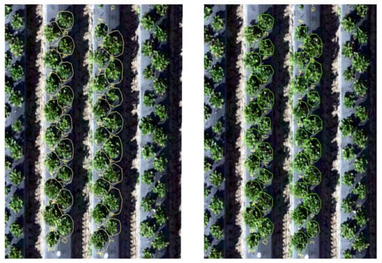
Figure 5.
Example of visually interpreted (left) and automatically delineated (right) canopies of plot 11 captured on 18 January 2017.
Visual interpretation of the canopies was a time-consuming process. A well-trained operator could take 2–3 h to delineate the 34 canopies in two plots and would still be vulnerable to errors, especially close to the end of the season when the canopies overlapped. The automated canopy-delineation approach took 15 min on average for each week’s dataset to process for all 34 plots using an Intel ®Xeon® CPU E3-1270 v5 @3.6 GHZ processor and 64 GB RAM computer.
Visual inspection of the automatically delineated canopy boundaries was required. Our review of the results showed the need to adjust the boundaries of a few canopies for each acquisition date, especially in the first and last acquisition dates when the canopies were either very small or overlapping, respectively. Additionally, although the developed workflow attempted to overcome the problems associated with increased weeds growing from the soils next to the beds at the end of the season, there were still some situations where automated delineation, and to a lesser extent visual interpretation, were affected by this situation. Visual review of the automatically delineated canopies and the potential editing of 2–3 canopies added up to 10 min to the processing time for each data acquisition (weekly) dataset.
Computing the canopy area, average height, standard deviation of canopy height, and canopy volume metrics was only conducted automatically using the developed canopy size metrics extraction geoprocessing workflow. The analysis was conducted for the whole dataset by iterating the model through all acquired datasets. The workflow was implemented as an ArcGIS software model since a step-by-step implementation using individual geoprocessing tools was impractical for multiple acquisition dates. Extracting canopy size metrics for each acquisition date took around 15 min using the same machine used for canopy delineation.
4.2. Manual and Automated Canopy Metrics Comparison
Four canopy metrics were computed using visually interpreted canopies and canopy boundaries derived using the automated workflow developed in this study. The difference between canopy metrics for each plant was computed. Statistical summaries of the differences for all the plants observed each week are shown in Figure 6. The figure shows a downward trend in the differences between canopy areas delineated through visual interpretation and automatically as the season progresses. The larger differences observed early in the season can be attributed to poor performance of the automated canopy delineation method in the first few weeks, when the plants included only a few dispersed leaflets. One of the steps to generate the canopies automatically applied a generalization process and fitted a minimum convex hull polygon to represent the canopy, which artificially distorted canopy boundaries. This distortion tended to be more severe early in the season resulting in smaller canopy sizes than for the visual interpretation process.
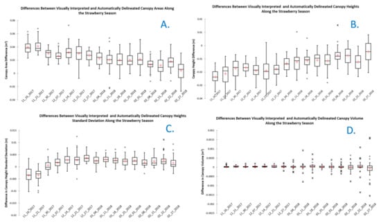
Figure 6.
Difference between canopy metrics derived using visually interpreted and automatically delineated canopy boundaries. (A). Differences in canopy area; (B). differences in average canopy height); (C). differences in canopy height standard deviation; and (D). differences in canopy volume.
Figure 6 also shows a trend of decreasing differences between average canopy heights and standard deviation of canopy heights derived from visually interpreted and automatically delineated canopies as the season progressed. This can be attributed to the same causes affecting the automatically delineated canopy areas earlier in the season. The mean values of canopy volume differences were consistently close to zero throughout the season. Large dispersion in volume differences was observed in the last weeks of the season. These observations included the largest canopy size of the season, where canopies grew significantly and overlapped with each other. This could have led to errors in the watershed canopy delineation results as canopy interference made it more difficult to find the boundaries of the canopies. Difficulties in making canopy boundary decisions were also reported in visually interpreted canopies at the end of the season due to canopy interference. Additionally, close to the end of the season, canopies continued to grow beyond the top surface of the bed and weeds grew from the soils between the beds towards the bed surface. Although we attempted to eliminate this effect by limiting the analysis to the boundaries of the bed tops, slivers of weed vegetation were still observed within some of the delineated canopies.
4.3. Biomass Modeling Using Canopy Size Variables
All four canopy size metrics used to model dry weight biomass were found to be statistically significant (p < 0.05). The variation inflation factor (VIF), a measure of multicollinearity, of the canopy volume variable, however, was found to be very high (20.03 and 20.3 for the automated and visually interpreted datasets, respectively). When the canopy volume variable was excluded and only the canopy area, average height, and standard deviation of the height variables were used, the VIF dropped significantly for all variables to a maximum of 7.04 (visually interpreted canopies dataset) and 5.4 (automatically delineated canopies) reported for the standard deviation of canopy height variable. All three variables of the two models and the intercept were significant (p < 0.001). The R2 values of the models were 0.77 and 0.76 for the automated and visually interpreted datasets, respectively. The LOO cross validation RMSE of the two models were 9.2 g and 9.4 g, respectively.
Table 3 shows the R2 and RMSE of the LGO cross validation results when the acquisition date and genotype groupings were used, respectively. The R2 values were computed for the models developed after excluding samples belonging to specific groups (acquisition date or genotype group) of observations. The RMSE was computed using the predicted and measured dry biomass of the excluded group samples. All the models were significant (p < 0.05). All the models showed that canopy area was significant (p < 0.05), while the other two metrics were not found consistently significant (p > 0.05) in all developed models.
Table 3.
Results of leave-acquisition (left) and leave-genotype (right) date-group cross validation of dry biomass models using canopy size metrics derived by automatically delineated and visually interpreted canopies.
5. Discussion
Automated raster analysis processes to delineate and extract canopy size metrics were applied to high spatial resolution images of strawberries throughout the Florida winter growing season. Although there were some differences between the canopy size metrics extracted using visually interpreted and automatically delineated canopies, these differences did not have a significant effect on the statistical models of dry biomass weight. The automated canopy delineation process utilized certain thresholds in the implementation that could be specific to certain field configurations, crop types, and image characteristics. For example, the mesh size and quantile elevation used to determine soils elevation within each mesh cell could be varied based on the configuration of the field (e.g., dimension of the elevated beds, spacing between the beds, field topography, etc.). These thresholds were tested and used consistently for the whole season and could be used repeatedly across seasons as long as the same bed configuration was maintained.
Visual inspection of automatically delineated canopies revealed the need to edit canopy boundaries for a few plants per acquisition date. This step was important early in the season, when some of the steps in the workflow, such as fitting the minimum bounding convex hull polygon, caused severe distortion in small canopy boundaries. Similarly, the weeds growing from the soils next to the beds and intruding onto the bed surface and the interference among adjacent canopies caused delineation errors close to the end of the season. Although adopting a consistent workflow throughout the season may have had some advantages for ease-of-use, the developed workflow could be improved by, for example, using thresholds driven by canopy age or genotype. Additionally, some functions such as canopy boundary generalization and convex hull fitting could be eliminated or modified to balance accuracy and aesthetic appeal of the resulting canopy.
Our geoprocessing analysis demonstrated the feasibility of using spatial interpolation methods to produce bare soil and bed surface from non-vegetation points and to use this surface as a digital terrain model to produce canopy-only 3D datasets. We utilized spatial interpolation with a strong directional emphasis so that the interpolated locations were only affected by the points in certain directions (along-bed direction). This was necessary since interpolation in all directions would have led to erroneous surfaces in a complex agricultural field like the ones used for strawberries. Another technique that was adopted to filter out weed vegetation growing from the soils onto the bed was to consider the vegetation above the bed elevation. Since the field was not flat, a mesh was used to determine soil elevation with each mesh cell, and bed elevation was determined by adding bed height to soil elevation within each mesh. This technique was efficient in eliminating the majority of the weeds. However, some weeds climbed above the bed surface towards the end of the season and affected the extracted canopy size metrics. Although only a few canopies suffered from this issue, further improvement could be achieved by attempting to filter out the weeds using spectral and textural information of the images.
Both LGO cross validation results showed consistent coefficient of determination R2 values (0.76–0.78 for genotype and 0.76–0.81 for acquisition date groups) regardless of canopy delineation methods. Some cross-validation groups, however, produced relatively high values, which might indicate that the model could fit certain groups (e.g., genotypes) better than others or that the canopy metrics extraction methods need to be fine-tuned to achieve better performance for some groups. Since our main objectives in this study were to compare model results based on automated and visual canopy delineation methods and to demonstrate automated geoprocessing workflow to analyze image data, only one of the simplest forms of statistical analysis, multiple regression, was used. This simple analysis technique produced reasonable fitting results; however, alternative analysis methods such as machine learning algorithms might lead to better prediction of dry biomass.
The workflows introduced in this process were successfully implemented on thousands of strawberry canopies to extract traits used in a genotyping experiment throughout two successive seasons. The details and the results of this experiment and its genetic implications were outside the scope of this manuscript and will be the subject of a future study. Although, using very high spatial resolution ground-based imagery was successful in extracting canopy size metrics and modeling dry biomass, capturing these images required installation of the sensors on field equipment and was relatively time-consuming. More experiments are planned using coarser-resolution drone-based imagery, which is more efficient and less demanding logistically. Moreover, including spectral information in the workflow to improve strawberry biophysical parameter estimation and provide additional vegetation traits to assist the strawberry breeding program is an undergoing effort by the research team.
6. Conclusions
This manuscript introduced raster-based geospatial analysis methods for strawberry canopy delineation and size metric extraction. Geospatial analysis techniques to produce canopy height elevation models and limit weed effects were demonstrated using a phenotyping experiment involving 17 different strawberry genotypes. Images were acquired weekly for 16 consecutive weeks throughout the strawberry growing season. Strawberry dry biomass multiple linear regression prediction models were developed using automatically extracted canopy size metrics. Only three of the four tested canopy metrics (canopy area, canopy average height, and standard deviation of canopy height) were used in model development due to existing multicollinearity among the variables. Leave-one-out and leave-group-out cross validation showed minimal differences in the coefficient of determination and RMSE when using visually interpreted or automatically delineated canopies. The R2 values of the models were 0.77 and 0.76 for the automatically delineated and visually interpreted canopy datasets and the LOO cross validation RMSE of the two models were 9.2 g and 9.4 g, respectively. The R2 values and RMSE computed using different acquisition dates and genotypes varied slightly, which indicates the potential for using a global dry biomass weigh prediction model for the whole season and across several genotypes. More research is recommended to improve the developed geoprocessing workflow, use coarser resolution drone images, and utilize more sophisticated modeling algorithms instead of the multiple regression models used in the study.
Author Contributions
Conceptualization, A.A.-E.; methodology, A.A.-E.; software, A.A.-E.; validation, K.B., C.D., B.W., and V.W.; formal analysis, Z.G.; investigation, A.A.-E.; resources, V.W.; data curation, Z.G., C.D. and A.G.; writing—original draft preparation, A.A.-E.; writing—review and editing, K.B., B.W., and V.W.; visualization, K.B.; supervision, A.A.-E.; project administration, A.A.-E. and V.W.; funding acquisition, A.A.-E. and V.W. All authors have read and agreed to the published version of the manuscript.
Funding
This research received no external funding.
Acknowledgments
The authors would like to acknowledge the Gulf Coast Research and Education field technical support staff for their efforts in developing the data acquisition platform.
Conflicts of Interest
The authors declare no conflict of interest.
References
- Mulla, D.J. Twenty five years of remote sensing in precision agriculture: Key advances and remaining knowledge gaps. Biosyst. Eng. 2013, 114, 358–371. [Google Scholar] [CrossRef]
- Watts, A.C.; Bowman, W.S.; Abd-Elrahman, A.; Mohamed, A.; Wilkinson, B.E.; Perry, J.; Kaddoura, Y.O.; Lee, K. Unmanned Aircraft Systems (UASs) for Ecological Research and Natural-Resource Monitoring (Florida). Ecol. Restor. 2008, 26, 13–14. [Google Scholar] [CrossRef]
- Liu, H.; Zhu, H.; Li, Z.; Yang, G. Quantitative analysis and hyperspectral remote sensing of the nitrogen nutrition index in winter wheat. Int. J. Remote Sens. 2019, 41, 858–881. [Google Scholar] [CrossRef]
- Xu, Y.; Smith, S.E.; Grunwald, S.; Abd-Elrahman, A.; Wani, S.P. Incorporation of satellite remote sensing pan-sharpened imagery into digital soil prediction and mapping models to characterize soil property variability in small agricultural fields. ISPRS J. Photogramm. Remote Sens. 2017, 123, 1–19. [Google Scholar] [CrossRef]
- Zhang, L.; Zhang, H.; Niu, Y.; Han, W. Mapping Maize Water Stress Based on UAV Multispectral Remote Sensing. Remote Sens. 2019, 11, 605. [Google Scholar] [CrossRef]
- Gerhards, M.; Schlerf, M.; Rascher, U.; Udelhoven, T.; Juszczak, R.; Alberti, G.; Miglietta, F.; Inoue, Y. Analysis of Airborne Optical and Thermal Imagery for Detection of Water Stress Symptoms. Remote Sens. 2018, 10, 1139. [Google Scholar] [CrossRef]
- Guo, C.; Zhang, L.; Zhou, X.; Zhu, Y.; Cao, W.; Qiu, X.; Cheng, T.; Tian, Y. Integrating remote sensing information with crop model to monitor wheat growth and yield based on simulation zone partitioning. Precis. Agric. 2017, 19, 55–78. [Google Scholar] [CrossRef]
- Chivasa, W.; Mutanga, O.; Biradar, C. Application of remote sensing in estimating maize grain yield in heterogeneous African agricultural landscapes: A review. Int. J. Remote Sens. 2017, 38, 6816–6845. [Google Scholar] [CrossRef]
- Newton, I.H.; Islam, A.F.M.T.; Islam, A.K.M.S.; Islam, G.M.T.; Tahsin, A.; Razzaque, S. Yield Prediction Model for Potato Using Landsat Time Series Images Driven Vegetation Indices. Remote Sens. Earth Syst. Sci. 2018, 1, 29–38. [Google Scholar] [CrossRef]
- Watanabe, K.; Guo, W.; Arai, K.; Takanashi, H.; Kajiya-Kanegae, H.; Kobayashi, M.; Yano, K.; Tokunaga, T.; Fujiwara, T.; Tsutsumi, N.; et al. High-Throughput Phenotyping of Sorghum Plant Height Using an Unmanned Aerial Vehicle and Its Application to Genomic Prediction Modeling. Front. Plant Sci. 2017, 8, 421. [Google Scholar] [CrossRef]
- Jang, G.; Kim, J.; Yu, J.-K.; Kim, H.-J.; Kim, Y.; Kim, D.-W.; Kim, K.-H.; Lee, C.W.; Chung, Y.S. Review: Cost-Effective Unmanned Aerial Vehicle (UAV) Platform for Field Plant Breeding Application. Remote Sens. 2020, 12, 998. [Google Scholar] [CrossRef]
- Chawade, A.; Van Ham, J.; Blomquist, H.; Bagge, O.; Alexandersson, E.; Ortiz, R. High-Throughput Field-Phenotyping Tools for Plant Breeding and Precision Agriculture. Agronomy 2019, 9, 258. [Google Scholar] [CrossRef]
- Pinter, J.P.J.; Hatfield, J.L.; Schepers, J.S.; Barnes, E.M.; Moran, M.S.; Daughtry, C.S.; Upchurch, D.R. Remote Sensing for Crop Management. Photogramm. Eng. Remote Sens. 2003, 69, 647–664. [Google Scholar] [CrossRef]
- Zhong, Y.; Wang, X.; Xu, Y.; Jia, T.; Cui, S.; Wei, L.; Ma, A.; Zhang, L. MINI-UAV borne hyperspectral remote sensing: A review. In Proceedings of the 2017 IEEE International Geoscience and Remote Sensing Symposium (IGARSS), Fort Worth, TX, USA, 23–28 July 2017; pp. 5908–5911. [Google Scholar]
- Yuan, H.; Yang, G.; Li, C.; Wang, Y.; Liu, J.; Yu, H.; Feng, H.; Xu, B.; Zhao, X.; Yang, X. Retrieving Soybean Leaf Area Index from Unmanned Aerial Vehicle Hyperspectral Remote Sensing: Analysis of RF, ANN, and SVM Regression Models. Remote Sens. 2017, 9, 309. [Google Scholar] [CrossRef]
- Clerici, N.; Rubiano, K.; Abd-Elrahman, A.; Hoestettler, J.M.P.; Escobedo, F.J. Estimating Aboveground Biomass and Carbon Stocks in Periurban Andean Secondary Forests Using Very High Resolution Imagery. Forests 2016, 7, 138. [Google Scholar] [CrossRef]
- Zhao, H.; Xu, L.; Jiang, H.; Shi, S.; Chen, D. HIGH THROUGHPUT SYSTEM FOR PLANT HEIGHT AND HYPERSPECTRAL MEASUREMENT. Int. Arch. Photogramm. Remote Sens. Spat. Inf. Sci. 2018, 42, 2365–2369. [Google Scholar] [CrossRef]
- Huang, P.; Luo, X.; Jin, J.; Wang, L.; Zhang, L.; Liu, J.; Zhang, Z. Improving High-Throughput Phenotyping Using Fusion of Close-Range Hyperspectral Camera and Low-Cost Depth Sensor. Sensors 2018, 18, 2711. [Google Scholar] [CrossRef] [PubMed]
- Guan, Z.; Abd-Elrahman, A.; Fan, Z.; Whitaker, V.M.; Wilkinson, B. Modeling strawberry biomass and leaf area using object-based analysis of high-resolution images. ISPRS J. Photogramm. Remote Sens. 2020, 163, 171–186. [Google Scholar] [CrossRef]
- Palace, M.; Sullivan, F.B.; Ducey, M.J.; Treuhaft, R.N.; Herrick, C.; Shimbo, J.Z.; Mota-E-Silva, J. Estimating forest structure in a tropical forest using field measurements, a synthetic model and discrete return lidar data. Remote Sens. Environ. 2015, 161, 1–11. [Google Scholar] [CrossRef]
- Wu, X.; Shen, X.; Cao, L.; Wang, G.; Cao, F. Assessment of Individual Tree Detection and Canopy Cover Estimation using Unmanned Aerial Vehicle based Light Detection and Ranging (UAV-LiDAR) Data in Planted Forests. Remote Sens. 2019, 11, 908. [Google Scholar] [CrossRef]
- Ke, Y.; Quackenbush, L.J. A review of methods for automatic individual tree-crown detection and delineation from passive remote sensing. Int. J. Remote Sens. 2011, 32, 4725–4747. [Google Scholar] [CrossRef]
- Jing, L.; Hu, B.; Noland, T.; Li, J. An individual tree crown delineation method based on multi-scale segmentation of imagery. ISPRS J. Photogramm. Remote Sens. 2012, 70, 88–98. [Google Scholar] [CrossRef]
- Marasigan, R.; Festijo, E.; Juanico, D.E. Mangrove Crown Diameter Measurement from Airborne Lidar Data using Marker-controlled Watershed Algorithm: Exploring Performance. In Proceedings of the 2019 IEEE 6th International Conference on Engineering Technologies and Applied Sciences (ICETAS), Kuala Lumpur, Malaysia, 20–21 December 2019; pp. 1–7. [Google Scholar]
- Chen, Q.; Baldocchi, D.; Gong, P.; Kelly, M. Isolating Individual Trees in a Savanna Woodland Using Small Footprint Lidar Data. Photogramm. Eng. Remote Sens. 2006, 72, 923–932. [Google Scholar] [CrossRef]
- Meyer, F.; Beucher, S. Morphological segmentation. J. Vis. Commun. Image Represent. 1990, 1, 21–46. [Google Scholar] [CrossRef]
- Huang, H.; Li, X.; Chen, C. Individual Tree Crown Detection and Delineation from Very-High-Resolution UAV Images Based on Bias Field and Marker-Controlled Watershed Segmentation Algorithms. IEEE J. Sel. Top. Appl. Earth Obs. Remote Sens. 2018, 11, 2253–2262. [Google Scholar] [CrossRef]
- Bao, Y.; Gao, W.; Gao, Z. Estimation of winter wheat biomass based on remote sensing data at various spatial and spectral resolutions. Front. Earth Sci. China 2009, 3, 118–128. [Google Scholar] [CrossRef]
- Zheng, H.; Cheng, T.; Zhou, M.; Li, D.; Yao, X.; Tian, Y.; Cao, W.; Zhu, Y. Improved estimation of rice aboveground biomass combining textural and spectral analysis of UAV imagery. Precis. Agric. 2018, 20, 611–629. [Google Scholar] [CrossRef]
- Maimaitijiang, M.; Sagan, V.; Sidike, P.; Maimaitiyiming, M.; Hartling, S.; Peterson, K.T.; Maw, M.J.; Shakoor, N.; Mockler, T.; Fritschi, F.B. Vegetation Index Weighted Canopy Volume Model (CVMVI) for soybean biomass estimation from Unmanned Aerial System-based RGB imagery. ISPRS J. Photogramm. Remote Sens. 2019, 151, 27–41. [Google Scholar] [CrossRef]
- Bendig, J.; Bolten, A.; Bennertz, S.; Broscheit, J.; Eichfuss, S.; Bareth, G. Estimating Biomass of Barley Using Crop Surface Models (CSMs) Derived from UAV-Based RGB Imaging. Remote Sens. 2014, 6, 10395–10412. [Google Scholar] [CrossRef]
- Brocks, S.; Bareth, G. Estimating Barley Biomass with Crop Surface Models from Oblique RGB Imagery. Remote Sens. 2018, 10, 268. [Google Scholar] [CrossRef]
- Abd-Elrahman, A.; Pande-Chhetri, R.; Vallad, G.E. Design and Development of a Multi-Purpose Low-Cost Hyperspectral Imaging System. Remote Sens. 2011, 3, 570–586. [Google Scholar] [CrossRef]
- Abd-Elrahman, A.; Sassi, N.; Wilkinson, B.; DeWitt, B. Georeferencing of mobile ground-based hyperspectral digital single-lens reflex imagery. J. Appl. Remote Sens. 2016, 10, 14002. [Google Scholar] [CrossRef]
- Roberts, J.W.; Koeser, A.K.; Abd-Elrahman, A.; Wilkinson, B.; Hansen, G.; Landry, S.M.; Perez, A. Mobile Terrestrial Photogrammetry for Street Tree Mapping and Measurements. Forests 2019, 10, 701. [Google Scholar] [CrossRef]
- Jensen, J.L.R.; Mathews, A.J. Assessment of Image-Based Point Cloud Products to Generate a Bare Earth Surface and Estimate Canopy Heights in a Woodland Ecosystem. Remote Sens. 2016, 8, 50. [Google Scholar] [CrossRef]
- Wolf, D.; Dewitt, B.A. Elements of Photogrammetry with Applications in GIS; McGraw-Hill: New York, NY, USA, 2000. [Google Scholar]
- Westoby, M.J.; Brasington, J.; Glasser, N.F.; Hambrey, M.J.; Reynolds, J.M. ‘Structure-from-Motion’ photogrammetry: A low-cost, effective tool for geoscience applications. Geomorphology 2012, 179, 300–314. [Google Scholar] [CrossRef]
- Triggs, B.; McLauchlan, P.F.; Hartley, R.I.; Fitzgibbon, A.W. Bundle Adjustment—A Modern Synthesis. Int. Workshop Vis. Algorithms 1999, 1883, 298–372. [Google Scholar]
- Liu, T.; Abd-Elrahman, A. An Object-Based Image Analysis Method for Enhancing Classification of Land Covers Using Fully Convolutional Networks and Multi-View Images of Small Unmanned Aerial System. Remote Sens. 2018, 10, 457. [Google Scholar] [CrossRef]
- Agisoft LLC. Agisoft PhotoScan User Manual: Professional Edition; Agisoft LLC: Saint Petersburg, Russia, 2016. [Google Scholar]
- Crippen, R. Calculating the vegetation index faster. Remote Sens. Environ. 1990, 34, 71–73. [Google Scholar] [CrossRef]
- Sirmacek, B. Shadow Detection. Available online: https://www.mathworks.com/matlabcentral/fileexchange/56263-shadow-detection (accessed on 19 September 2020).
- Sirmacek, B.; Ünsalan, C. Damaged building detection in aerial images using shadow Information. In Proceedings of the 2009 4th International Conference on Recent Advances in Space Technologies, Istanbul, Turkey, 11–13 June 2009; pp. 249–252. [Google Scholar]
- Joblove, G.H.; Greenberg, D. Color spaces for computer graphics. In Proceedings of the 5th Annual Conference on Computer Graphics and Interactive Techniques, New York, NY, USA, 23–25 August 1978; pp. 20–25. [Google Scholar]
- Bar-On, Y.M.; Phillips, R.; Milo, R. The biomass distribution on Earth. Proc. Natl. Acad. Sci. USA 2018, 115, 6506–6511. [Google Scholar] [CrossRef]
- Plowright, A.; Roussel, J.-R. ForestTools: Analyzing Remotely Sensed Forest Data. Available online: https://rdrr.io/cran/ForestTools/ (accessed on 19 September 2020).
- ESRI. ArcMap. Available online: https://desktop.arcgis.com/en/arcmap/ (accessed on 19 September 2020).


Publisher’s Note: MDPI stays neutral with regard to jurisdictional claims in published maps and institutional affiliations. |
© 2020 by the authors. Licensee MDPI, Basel, Switzerland. This article is an open access article distributed under the terms and conditions of the Creative Commons Attribution (CC BY) license (http://creativecommons.org/licenses/by/4.0/).