Crop Type Classification Using Fusion of Sentinel-1 and Sentinel-2 Data: Assessing the Impact of Feature Selection, Optical Data Availability, and Parcel Sizes on the Accuracies

Abstract

Crop type classification using Earth Observation (EO) data is challenging, particularly for crop types with similar phenological growth stages. In this regard, the synergy of optical and Synthetic-Aperture Radar (SAR) data enables a broad representation of biophysical and structural information on target objects, enhancing crop type mapping. However, the fusion of multi-sensor dense time-series data often comes with the challenge of high dimensional feature space. In this study, we (1) evaluate how the usage of only optical, only SAR, and their fusion affect the classification accuracy; (2) identify the combination of which time-steps and feature-sets lead to peak accuracy; (3) analyze misclassifications based on the parcel size, optical data availability, and crops’ temporal profiles. Two fusion approaches were considered and compared in this study: feature stacking and decision fusion. To distinguish the most relevant feature subsets time- and variable-wise, grouped forward feature selection (gFFS) was used. gFFS allows focusing analysis and interpretation on feature sets of interest like spectral bands, vegetation indices (VIs), or data sensing time rather than on single features. This feature selection strategy leads to better interpretability of results while substantially reducing computational expenses. The results showed that, in contrast to most other studies, SAR datasets outperform optical datasets. Similar to most other studies, the optical-SAR combination outperformed single sensor predictions. No significant difference was recorded between feature stacking and decision fusion. Random Forest (RF) appears to be robust to high feature space dimensionality. The feature selection did not improve the accuracies even for the optical-SAR feature stack with 320 features. Nevertheless, the combination of RF feature importance and time- and variable-wise gFFS rankings in one visualization enhances interpretability and understanding of the features’ relevance for specific classification tasks. For example, by enabling the identification of features that have high RF feature importance values but are, in their information content, correlated with other features. This study contributes to the growing domain of interpretable machine learning.

1. Introduction

Crop type maps deliver essential information for agricultural monitoring and are likewise relevant for other fields such as environmental assessments. Respective classification approaches using Earth Observation (EO) stand to benefit from the availability of high-resolution Sentinel-1 and Sentinel-2 dense time series. Particularly, the synergistic use of these optical and Synthetic-Aperture Radar (SAR) datasets bears high potential. In previous research, single-sensor approaches based on optical and SAR data were used the most to map crop types at different scales. A larger share of research was based on optical data [1,2,3,4,5]. The classification of crop types using only SAR data has also been successfully implemented in several studies [6,7,8,9]. Optical data that makes use of the visible, near-infrared, and short-wave-infrared portion of the electromagnetic spectrum, provides valuable information about leaf pigments, water content, and plants’ overall health condition.; whereas SAR data, dependent on the frequency and polarization, delivers a complex representation of canopy structure, surface roughness, soil moisture, and topography [10].

The first studies that focused on optical-SAR data fusion date back to the 80s [11,12]. However, starting from 2000, the number of studies on this topic gradually increased, which can be partially explained by the launch of new space-borne radar (ERS, RADARSAT, ENVISAR, ASAR, etc.) and optical (Landsat, SPOT, IRS, MODIS, QuickBird, etc.) satellites [13]. The launch of Sentinel-1 (2014/2016) and Sentinel-2 (2015/2017), operated by the European Space Agency (ESA), boosted the interest in using these freely available SAR and optical datasets for crop type mapping in a synergistic way. Optical and SAR data’s complementary nature gives the possibility to simultaneously utilize information on plants’ structural and bio-physical conditions. This explains that most previous fusion studies reported improvements in crop classification accuracy when optical and SAR data were combined compared to single sensor experiments [14,15,16]. Commonly, optical-SAR fusion studies used several cloud-free optical and available SAR scenes for their studies [13]. The use of dense time-series of both became more common in recent studies [17,18]. However, for large-scale studies, it is still a challenge to combine these two datasets since vast volumes of diverse datasets demand higher processing power and resources.

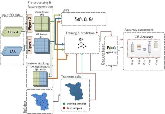
There are three primary data fusion levels: pixel-level, feature-level (further, feature stacking), and decision-level [19] (for details see Section 2.4.1). Among crop type classification studies, Gibril et al. [20] compared pixel-level fusion techniques (Brovey Transform, Wavelet Transform, Ehlers) with feature stacking results. To the best of our knowledge, the comparison between optical-SAR feature stacking and optical-SAR fusion at decision-level was not subject to any study even though decision fusion was successfully applied [21]. Multi-sensor feature stacking may result in high dimensional feature space, which may negatively affect the classification accuracy. While decision fusion, based on classification confidences derived from single sensor predictions, might profit from less complex models. It could be valid to expect that optical-SAR fusion at the decision-level could be more performant than simple feature stacking. To test this hypothesis, in this study, we compare the classification results derived from optical-SAR feature stacking and optical-SAR fusion at decision-level (further, decision fusion).

Combining dense optical and SAR time series features can quickly result in a high-dimensional feature space that can pose challenges for pattern recognition and machine learning. In terms of classification accuracy, earlier methods such as the parametric maximum likelihood classifier are more susceptible to high-dimensional feature spaces than to state-of-the-art classifiers, such as Support Vector Machines and Random Forest (RF). Nevertheless, studies have shown that these classifiers’ accuracy can also be increased by feature selection [22], particularly when the amount of training samples is limited [23]. Elaborated pre-processing, feature generation, and selection of suitable features are needed for many classification algorithms. Commonly derived features as spectral-temporal variability metrics [24], time-weighted interpolation [5], or computationally more expensive approaches such as time-weighted dynamic time warping [25] are being used less often for large-scale applications. This happens probably due to, among other reasons, high computational complexity, particularly over very large areas.

Feature selection methods have a long tradition in pattern recognition analysis of remote sensing data [26,27], alleviating the challenges mentioned earlier. It helps to train more accurate models, decrease computational complexity, and improve the understanding of the used features [28,29]. Data and model understanding is essential in the development of operational products [30] and in scientific research where feature importance and rankings are often essential elements [28,31,32]. The main groups of feature selection are filters and wrappers methods [33]. Filter methods use various statistical measures (e.g., Chi-square test, Pearson’s correlation) to score the relevance of features. Whereas, wrapper methods perform feature selection based on the chosen classifiers’ performance, which enables to select most performant features with low correlation. The main drawback of the wrapper approaches is the high computational costs. In crop type classification studies, embedded methods such as classifier specific RF feature importance is often used to select the most important features [34]. It is a fast approach, but a drawback is that features with correlating information content can show similarly high importance scores.

To alleviate the limitations of wrapper methods concerning high computing efforts, in this study, we perform a group-wise forward feature selection (gFFS). gFFS allows focusing the analysis and interpretation on useful feature sets like spectral bands, vegetation indices (VIs), or data acquisition dates (for details see Section 2.4.3). A similar approach was followed by Defourny et al. [35]. The grouping strategies of features in the gFFS have two important benefits: (1) gFFS allows to tailor the feature selection towards better interpretability and supports a more efficient feature selection process. For example, the time-steps with most discriminative power can be better analyzed by considering all information available at a particular time-step as a group and not only as single features. (2) gFFS allows the substantially reduced computational time of the feature selection step while considering all features at hand.

In addition to an appropriate feature selection, the quality of the satellite data features concerning data availability and gaps are crucial aspects that can influence classification accuracy. Croplands are typically characterized by management activities such as tilling, sowing, and harvesting or cutting and are, therefore, amongst the most dynamic land cover elements. Their successful identification via remote sensing data often requires dense time-series information capable of capturing critical plant development phases and the mentioned land management activities [36]. The comparison of seasonal, monthly composites, and gap-filled Harmonized Landsat and Sentinel-2 [37] time-series (10-days interval) data by Griffiths et al. [4] showed that the highest classification performance was achieved with gap-filled 10-day time-series data. However, the quality of the gap-filled data depends on the duration and number of gaps. Gaps originate mainly from cloud cover, cloud shadows, and other atmospheric effects from which optical data are often suffering. In this sense, combining dense time series of SAR features and gap-filled optical data could result in more accurate classifications.

In summary, despite the large number of studies focusing on the combination of optical and SAR features for crop type mapping, the following aspects were not sufficiently investigated: (1) combined performance of a comparably high number of relevant Sentinel-2 and Sentinel-1 dense time-series features for larger areas covering more than one sensor swath, where the derivation of spatially homogeneous features across all the study area is required; (2) impact of optical-SAR feature stacking and decision fusion on classification accuracies; (3) analysis and interpretation of feature importance and ranking based on dates, bands, and VIs instead of single features and their effect on classification accuracies; (4) the performance of respective classification approaches to differentiate 16 crop types; (5) analysis of the influence of the optical data availability, parcel size, and pixel location within the parcel on the classification results.

This study aims to contribute to these open issues by evaluating how the synergetic use of dense optical and SAR time-series data derived from Sentinel-1 and Sentinel-2 improves the classification accuracy of typical crop types of Central Europe. The study site covers the Brandenburg state, located in northern Germany. In this context, we investigate how a large number of optical and SAR features affect the performance of RF models and evaluate the relevance of various feature-sets and time-steps to the classifier. It is also analyzed how agricultural parcel size, mixed pixels occurrence at parcel borders, and the non-availability of optical satellite data at specific dates of the year affect the classification accuracy. More explicitly, the following questions were addressed:

• How do the usage of single-sensor dense time-series data and the fusion of Sentinel-1 and Sentinel-2 data affect the classification accuracy? Do classification accuracies based on optical-SAR feature stacking differ from decision fusion?
• How does a high dimensionality of optical-SAR feature stack impact on the performance of RF? Which features are most relevant, and which dates and bands or VIs lead to the highest accuracies?
• What is the influence of cloud-related gaps in optical data, how do parcel sizes, and the pixel location within a parcel affect classification accuracy?

2. Materials and Methods

2.1. Study Area

The study site (Figure 1) is located in Northern Germany and covers the territory of Brandenburg state with an area of 29,654 km², where 45% is agricultural land [38]. Large-scale farms dominate the state croplands with 238 ha of average field size [38]. The area has low topographic complexity with the highest peak in the state being at 201 m.a.s.l. (Kutschenberg hill) and the lowest point is Rüdersdorfer opencast mining area with −46.5 m below sea level. The average annual precipitation is 719 mm, and the average annual temperature is 9.9 °C. Winter cereals are sown at the beginning of September and harvested at the end of July and beginning of August. Summer crops are sown at the end of March—beginning of April and harvested at the end of July—beginning of August [39].

2.2. Reference Data

As ground truth data on crop types for the year 2017, we used reference data from the Brandenburg Surveying and Geospatial Information Office (Landesvermessung und Geobasisinformation Brandenburg) web-portal [40]. This reference parcel data, managed by Land Parcel Identification System (LPIS), is based on the reports of farmers who applied for agricultural subsidies in the frame of the European Union’s (EU) Common Agricultural Policy (CAP). Further, we refer to this dataset as LPIS. The data contains parcel boundaries and crop types harvested in the year 2017.

The original dataset is available in a geospatial vector format and contains 161,503 parcels. Overlapping parcels and parcels with an area less than 1000 m² were excluded from the reference data (1364 parcels, 3017.516 ha). Out of the 158 original crop types, several crop classes were merged into grouped classes based on their biological plant family membership and phenological similarity. For example, class maize includes silo maize, maize for biogas, maize with flowering path, etc., and class potatoes comprise starch potatoes and potatoes for food. Supplementary Material A gives an overview of the original and grouped classes. Only those grouped crop classes were selected from the original reference data, which accounted for at least 0.5% of the full LPIS area. The only exception was made for the class sugar beets, which areal cover was close to the threshold (0.46%). This resulted in 16 crop classes (

Table 1. Overview information for the crop types considered in this study.

Crop Type	Number of Parcels	Average Parcel Size [ha]
Permanent grasslands	59,182	4.94
Temporal grasslands	12,092	3.77
Maize	14,449	14.27
Sunflowers	834	12.26
Potatoes	1015	9.17
Sugar beets	240	24.86
Winter wheat	9758	17.59
Winter rye	14,117	11.45
Winter rape	6299	20.09
Winter barley	5189	17.36
Winter triticale	3289	11.01
Summer barley	934	7.49
Summer oat	2394	5.91
Legume mixture	2297	8.98
Peas-Beans	897	10.89
Lupins	1393	8.70

) for which a total of 134,379 parcels (1,220,160.86 ha) was available in the LPIS data. Since crop groups such as winter cereals (winter wheat, winter rye, winter rape, winter barley, winter triticale), summer cereals (summer barley, summer oat), and legumes (legume mixture, peas-beans, lupins) are expected to show high intra-class confusion, we additionally report the accuracy results when these classes are grouped into one. The present study focuses only on crop type classification. No other land cover land use classes were considered.

2.3. Remote Sensing Data Pre-Processing and Features Generation

The data sensed by the Multi-Spectral Instrument (MSI) onboard Sentinel-2A/B, and by the C-band synthetic aperture radar (SAR) instrument onboard Sentinel-1A/B were analyzed in this study. The data were accessed via The Copernicus Open Access Hub (https://scihub.copernicus.eu/). The tiling grid of Sentinel-2 data was used as a base grid (Figure 2.). Brandenburg’s entire territory is covered by eight Sentinel-2 tiles. Overall, 494 optical scenes and 473 SAR scenes (in ascending mode) were utilized with temporal coverage from the beginning of January until the end of September 2017. Optical data acquired in October were entirely excluded from the analysis due to the lack of any scene with cloud cover below 80%.

2.3.1. Optical Data Pre-Processing and Gap-Filling

The individual pre-processing steps that were applied to Sentinel-2 data are shown in Figure 3. Sentinel-2 data at Level-1C (top of atmosphere) were processed to Level-2A (bottom of atmosphere) using sen2cor v2.4.0 [41]. Ten Sentinel-2 bands were used for further analysis. Bands 1 (coastal aerosol), 9 (water vapor), and 10 (Short-Wave-Infrared (SWIR)-cirrus) were excluded from the analysis because of their irrelevance for crop type mapping. The data of the red-edge (5, 6, 7), near-infrared narrow (8A), and SWIR bands (11, 12) were resampled from 20 to 10 m spatial resolution using the nearest neighbor algorithm. In addition to the original Sentinel-2 bands, four well-known VIs were generated: Normalized Difference Vegetation Index (NDVI), Normalized Difference Water Index (NDWI), Normalized Difference Yellow Index (NDYI), and Plant Senescence Reflectance Index (PSRI) [42,43].

Cloud masks were produced in two steps. First, cloud masks were calculated using the fmask [44] extended for Sentinel-2 data, according to Frantz [45]. Second, we combined information from the Scene Classification Layer (SCL) generated by sen2cor [41] and the output of the fmask into a single binary invalid pixel mask. We flagged a pixel as invalid if at least one of these two input layers detected cloud, cloud shadow, snow, defect, saturated pixels.

Different acquisition times, clouds and cloud shadows lead to irregular time series of valid observations over the study area. Instead of using generic ways of handling missing data within RF [46], we build a consistent gap-free time series over the whole study site with time-weighted linear interpolation. It allows accounting better for the temporal information contained within the original satellite time series data. Dense time series were created based on invalid pixel masks, four VIs, and the 10 bands of Level-2A data at 10 m spatial resolution. Following the approach of Inglada et al. [5], gap-filling started by defining bi-weekly target dates from January to September 2017. In total, we defined 20 target dates. After applying the invalid pixel mask, band wise time-weighted linear interpolation was performed considering only valid pixels to fill the defined target dates.

2.3.2. SAR Data Pre-Processing

C-band Level-1 Ground Range Detected (GRD) Sentinel-1 products, acquired in Interferometric Wide (IW) swath mode, were accessed via the Google Earth Engine (GEE) platform [47]. The data available in GEE were pre-processed with the Sentinel-1 toolbox from ESA, which involved updating orbit metadata, thermal noise removal, radiometric calibration, and terrain correction. For the scenes in ascending mode, we filtered extreme incidence angles so that only observations with incidence angles of 32° to 42° were used. The average incidence angle in the study area is equal to 37°. Lee speckle filtering and square cosine correction were applied as it was outlined by Tricht et al. [17]. After the incidence angle correction, we calculated bi-weekly medians and matched the time steps to the 20-target time-series dates of the optical features (Figure 4).

2.4. Methodology

The methodological workflow of this study consists of the following steps (Figure 5): (1) extraction of optical and SAR time-series features at the pixel level (see Section 2.3 for more details); (2) sampling of training and testing pixels; (3) performing group-wise forward feature selection (gFFS), where individual features are grouped by time or variable respectively; (4) building RF models using all existing features and the best-performing feature subsets identified in (3); (5) predicting test-sets; (6) extracting accuracy metrics; (7) analyzing results using the information of RF feature importance and feature group ranking; (8) analyzing auxiliary data on the parcel size, optical data availability, temporal profiles of correctly and misclassified pixels.

2.4.1. Single Sensor Features Versus SAR-Optical Combination

To compare and evaluate the accuracy achieved with single sensor features and their fusion, we separately classified only optical features, only SAR features, and a fusion of optical and SAR features. As optical features (in plots shown as S2), we selected 10 Sentinel-2 spectral bands and four VIs, as described in Section 2.3.1. In total, 20 time-steps of 10 spectral bands and four VIs summed up to 280 optical features. As for SAR features (in plots shown as S1), bi-weekly medians of VV and VH bands were used (pre-processing steps in Section 2.3.2.). They summed up to 40 SAR features.

According to Pohl and van Genderen [19], there are three levels of data fusion: pixel-level, feature-level, and decision-level. At the pixel-level fusion, multi-sensor input data are fused into a new dataset using various compression, dimensionality reduction methods (e.g., Principal Component Analysis, Wavelet-based approaches, Brovey Transform) and then used for prediction or analysis. The feature-level fusion implies combining extracted features from different sensors to form a new multi-source feature stack. In this study, we will refer to this method as a feature stacking. Such multi-sensor feature stacking is more commonly used in crop type classification studies [13]. Joshi et al., [48] refers to these two data fusion levels as ‘pre-classification or -modeling fusion’. Whereas ‘post-classification or -modeling fusion’ would be a decision-level fusion, which is performed by fusing the classification results of single sensor features based on pre-delineated rules or decisions. In this study, we perform optical-SAR feature stacking and decision fusion.

The feature stacking was performed by stacking the abovementioned optical and SAR features into one optical-SAR feature stack (in plots shown as ff(S1&S2)). The decision fusion was done by fusing classifications derived from single-sensor features. We used the class probabilities of the RF to derive confidence values for S1 and S2, respectively. In the scikit-learn implementation of RF [49], the class probabilities were calculated as the mean predicted class probabilities of the trees in the forest. For a single tree, the class probability is defined by the fraction of samples of the same class in a leaf. The confidence level was calculated by the difference between the highest and second-highest class pseudo-probabilities. During decision fusion (in plots shown as df(S1&S2)), the prediction with the highest confidence level was selected as a final prediction.

2.4.2. Sampling Strategy

From the refined LPIS reference data (Section 2.2.), 50% of the parcels were selected for training, and 50% of the parcels for testing. Train-test split was done at the parcel level, to ensure that none of the test-set pixels come from a parcel which already was chosen for training. Training and testing pixels were not chosen within a buffer of 1 (10 m) pixel distance from parcel borders to avoid mixed spectral signatures. Training and testing pixels were sampled using equally stratified random sampling with 3000 samples size per crop type. This sample size was chosen to competently represent the spectral and phenological variability of the classes under investigation. It was ensured that training and testing pixels were equally sampled from small and large parcels to avoid underrepresentation of the small parcels. For each training and testing sample, information about the parcel size, the number of valid and invalid optical observations per month, and the sample’s distance to the parcel border was stored as auxiliary data. These datasets were further used for the analysis of the results (Section 3.3.).

2.4.3. Group-Wise forward Feature Selection

To evaluate the significance of the features and the effect of the high feature amounts on the accuracy of the RF classifier, we used a modified sequential forward feature selection (FFS) approach. FFS is one of the variations of the sequential feature selection (SFS) approach, which belongs to wrapper methods. The procedure starts with building several RF, each using only one of the available features (1st sequence). Based on the accuracies of these RFs, the best (e.g., in terms of accuracy) feature is selected and combined to sets of two features using all remaining features. Again, several RFs are generated, based on sets of two features (2nd sequence). This process is repeated, and with every iteration, a new feature is added until only one RF, including all features, is constructed. This is often done to get a full feature ranking and investigate if the accuracy decreases at a certain point while increasing dimensionality. Early stopping is also possible, e.g., by defining a desired number of features, by stopping when the peak performance is reached, or if the accuracy of a new iteration does not increase significantly compared to the previous iteration [50].

Wrapper methods such as FFS are computationally expensive and often impractical to perform when large amounts of features are used. It is particularly true for studies using dense time-series like the presented study. For example, to run a complete FFS with the 320 features considered in this study, it would need 51,360 model evaluation runs (Equation (1)), where one model evaluation comprises to train an RF, predict validation data, and calculate the accuracy of the model. Moreover, with 5-fold cross-validation, it sums up to 256,800 model evaluation runs (Equation (2)).

$${\displaystyle \sum }_{i=1}^{320}i =51,360$$

(1)

$${\displaystyle \sum }_{i=1}^{320}5i =256,800$$

(2)

Since the focus of our study is not to evaluate the significance of individual features but rather to understand which time steps or spectral bands, VIs, and backscattering coefficients contribute the most to the accuracy of the classification model, we modified FFS in a way that also reduced computational efforts (Figure 6). The modification was done by performing group-wise FFS (gFFS), where features are grouped based on a time-step (further, time-wise gFFS) and on a variable (further, variable-wise gFFS). For example, in time-wise gFFS, the group ‘07-May’ consists of 2 (VV, VH), 14 (all bands and VIs), and 16 (a combination of those) features in case of S1, S2, and ff(S1&S2), respectively. Whereas the variable-wise gFFS considers the full time-series of a particular band or index as one entity (e.g., NDVI full time-series, VH full time-series). As a base of gFFS, we used the core implementation of the sequential feature selection (SFS) available in the MLxtend python package [51]. In total, time-wise gFFS required 1050 model evaluations for only optical, only SAR, and a combination of optical and SAR features. Variable-wise gFFS required 15 runs for SAR, 525 runs for optical, and 680 runs for optical-SAR features. These numbers already include the five-fold cross-validation runs, which were applied for receiving more robust estimates.

2.4.4. Classification Approach

The classification process was performed using state-of-the-art remote sensing image classifier-RF algorithms. It is a non-parametric machine learning algorithm consisting of an ensemble of randomized decision trees [52]. Each decision tree predicts a target class for each training sample, and the class with the highest number of votes within the forest is selected as the ensemble’s final decision. Previous studies focusing on crop type mapping [5,53,54] show that RF produces generally accurate results. Due to its robustness to class label noise and high dimensional input data [34], it is extensively used in crop type classifications [15,30,55].

In our study, we used the scikit-learn Python implementation of the RF algorithm. Based on the results of a randomized search using a five-fold cross-validation [49], the following parameters were applied: (1) number of trees—700; (2) maximum depth—30; (3) maximum number of features used to split the node—square root of the sum of features; (4) minimum sample number to split a node—25.

The final RF models were built for optical, SAR, optical-SAR features using all features, and feature subsets selected based on the results of the time-wise and variable-wise gFFS (Section 2.4.3.). For all final RF models, the Gini importance score (also known as Mean Decrease in Impurity (MDI)) was used to evaluate the significance of the single features, further referred to as the RF feature importance. These feature importance scores were compared to the outcomes of the gFFS.

To assess and compare the classification accuracies, we computed class-specific metrics such as precision (i.e., user’s accuracy), recall (i.e., producer’s accuracy) and class-specific f1-score. The f1-score (Equation (3)) is a weighted average measure of precision and recall, where f1-score reaches the best values at 1 and worst values at 0. The average over the class-specific f1-scores has been computed to get a single accuracy metrics over all classes [49]. In addition, we calculated confusion matrices.

$$f1=2\ast \left(precision\ast recall\right)/\left(precision+recall\right)$$

(3)

Accuracies were calculated for all 16 classes. To understand how accuracy is impacted by expected confusion among cereal and legume crops, we also calculated grouped classification accuracy while treating cereals and legumes as one crop class.

2.4.5. Analysis of the Impact of Parcel Size, Pixel’s Location within a Parcel, Optical Data Availability on Classification Accuracy

As was mentioned in Section 2.4.2., for each training and testing sample, we stored the information about the parcel size from which it was sampled. This data was then used to plot parcel size distributions for mis- and correctly-classified test samples.

The pixel’s distance to the parcel border was calculated using the eo-box python package [56]. Further, testing samples from individual crop types were grouped based on the distance to parcel borders, and then for each group, f1-score was calculated. Because of the parcel size variations, the number of samples in each group varies. Especially for more considerable distances such as 30–40 pixels away from parcel border, the underlining number of pixels used to calculate f1-score could be minimal. This results in expected significant variations on large distances. In the plot, the red vertical line indicates the distance at which 80% of samples have already been used to calculate f1-scores. Depending on the parcel size distributions of each crop type, the red vertical line switches along the x-axis.

Using the invalid pixel mask (see Section 2.3.1.), we calculated the number of valid optical observations per month for each sample. The numbers varied from 0 to 5, where 0 means that no valid optical observation was available for considered samples at the specific month.

The temporal profiles were built using NDVI and VH values for mis- and correctly classified samples.

3. Results

3.1. Classification Accuracies (Overall and Class-Specific)

The f1-scores obtained from the predictions based on all features and the best-performing feature subsets selected using time-wise gFFS and variable-wise gFFS are shown in

Table 2. Classification accuracies (f1-score) based on all features and the features subsets selected based on time-wise and variable-wise gFFS after grouping legume and cereal classes.

	All Features	Subset (Variable-Wise gFFS)	Subset (Time-Wise gFFS)
S1	0.76	0.76	0.76
S2	0.73	0.73	0.73
ff(S1&S2)	0.81	0.81	0.80
df(S1&S2)	0.80	0.80	0.80

. The gFFS did not have any effect on the accuracy values for the experiments based on only SAR features (S1), optical features (S2), and decision fusion (df(S1&S2)). The decrease of f1-score by only 0.01 was recorded with time-wise gFFS for experiments based on optical-SAR features stacks (ff(S1&S2)). Also, in the class-specific accuracies, no significant changes were recorded (Supplementary Materials B). Based on these outcomes, we continue reporting classification accuracies based on the results when all the existing features were used.

The f1-score of the predictions based on S2 and S1 was equal to 0.61 and 0.67, respectively, without class-grouping. After grouping cereal and legume classes, f1-score derived from S2, and S1 classifications increased to 0.73 and 0.76, respectively. There was no significant difference in the mean precision and recall values for single sensor experiments (S2: precision—0.62, recall—0.61; S1: precision—0.68, recall—0.67).

The classifications based on ff(S1&S2) resulted in an f1-score of 0.72 with a precision of 0.73 and a recall of 0.72 without class-grouping. Decision fusion showed similar results (f1-score—0.71, precision—0.72, recall—0.72). Considering the grouped cereal and legume classes, f1-scores of both fusion approaches increased to 0.81, 0.80 for ff(S1&S2) and df(S1&S2) accordingly. Thus, both considered fusion approaches outperformed the single sensor accuracies.

Figure 7 gives an overview of the class-specific accuracies for a single sensor and fused feature results. In general, class-specific accuracies showed higher diversity compared to overall accuracies. Winter rape and sugar beet classes showed the best accuracy results (f1-score > 0.90), with only minor differences between the used sensors or fusion types.

Most crop types showed the highest accuracies when using ff(S1&S2), and were better classified with S1 compared to S2. For example, this applies to all winter cereals (winter rape, winter wheat, winter rye, winter barley, and winter triticale) with f1-scores > 0.70. The same pattern could be seen for summer cereals (summer barley and summer oat) and potatoes. Nevertheless, f1-scores remained below 0.6 for both summer cereals. Potatoes and maize had the highest f1-score with ff(S1&S2), which were 0.75 and 0.79. For classes such as sunflowers, lupins, and peas-beans, the performance of models built using S1 was quite close to the performance of the models built using ff(S1&S2) (f1-scores: ∆ = 0.03, ∆ = 0.03, ∆ = 0.01, accordingly) while using S2 resulted in slightly lower accuracies (f1-scores: ∆ = 0.18, ∆ = 0.21, ∆ = 0.19, accordingly). In contrast, the two considered grassland classes had higher classification accuracies when using S2 (f1-scores: temporal grasslands—0.42, permanent grasslands—0.62) compared to S1 (f1-scores: temporal grasslands—0.38, permanent grasslands—0.51). This can also be seen from the map presented in Figure 8. Nonetheless, for these classes, the maximum accuracy score is reached with fused datasets (f1-scores ff(S1&S2): temporal grasslands—0.45, permanent grasslands—0.64).

Permanent and temporal grasslands had a high within-group confusion rate (Figure 9). The test samples of legume mixture and temporal grasslands were often predicted as permanent grasslands, reflecting low precision and high recall values. Maize samples were often predicted correctly (recall = 86), but false predictions of sunflower, potato, and lupin samples as maize affected the precision, which was equal to 73. Summer and winter cereals formed two groups with high intra-group confusion. For winter cereals, higher confusion was present among classes such as winter wheat, winter rye, and winter triticale. Whereas, summer cereals were not only confused within the group but also often were classified as one of the legume classes. The confusion between summer cereals and legume classes are higher when using only optical feature compared to SAR only features. Supplementary Materials C includes all confusion matrices for all experiments.

After combing summer barley and summer oat (which were heavily confused, see Figure 10) into a single class of summer cereals, the f1-score increased to 0.78 with ff(S1&S2) (Figure 8). The classes lupins, peas-beans, and legume mixture, when grouped to one legumes class, got the highest f1-score of 0.77 with ff(S1&S2). The f1-score of class winter cereals raised above 0.90 with ff(S1&S2) after grouping. However, when merging classes, the general pattern, that optical-SAR feature combination and decision fusion were outperforming single sensor information, remained unchanged.

3.2. gFFS Rankings and Feature Importance

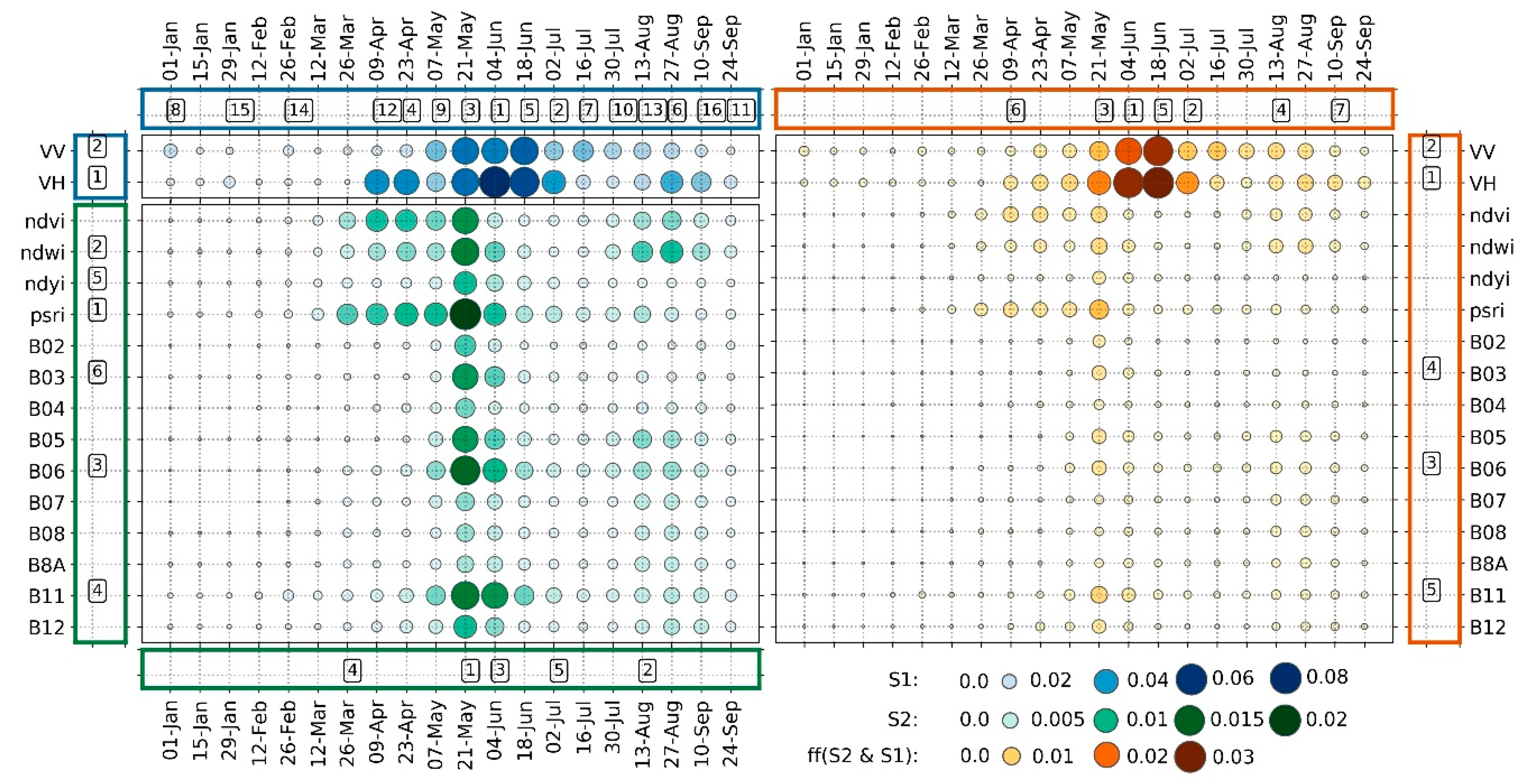
The RF model with the highest accuracy (f1-score: 0.7) was achieved using a variable-wise gFFS at the 5th sequence with 100 features with ff(S1&S2) (Figure 11). By variable-wise gFFS, the full time-series of VH, VV, red-edge (B06), green (B03), and SWIR (B11) were identified as the most performant feature-sets (Figure 12, border axis). The f1-score difference at the point with the maximum performance (100 features) and the last sequence (320 features) was only 0.01.

The time-wise gFFS showed the maximum performance (f1-score: 0.69) with 112 features at the 7th sequence with ff(S1&S2). The dates chosen as being most crucial by time-wise gFFS are shown in the border axis of Figure 12. No significant difference was observed between the maximum performance value and the f1-score at the last sequence with 320 features (∆ = 0.001).

When applied to only optical features, time-wise and variable-wise gFFS showed identical maximum accuracy results with f1-score of 0.58. The difference was in the number of features, where time-wise gFFS peaked at the 5th sequence with 70 features, and variable-wise gFFS peaked at the 6th sequence with 120 features.

The use of both, VH and VV feature-sets (40 features), showed the highest performance (f1-score: 0.65) of the variable-wise gFFS when applied to only SAR features. The maximum performance (f1-score: 0.66) of the time-wise gFFS for VV and VH features was achieved at the 16th sequence.

The RF importance scores derived from the RF models trained using optical (greens), SAR (blues), and optical-SAR feature stack (orange-brown) are illustrated in Figure 12. The experiments using only SAR features showed that data from April until mid-September were the most valuable for the classifier. The highest importance scores were given to the features acquired in June when the majority of crops are close to their full development stage. The results of those experiments that were based on only optical features showed that information obtained from three VIs (psri, ndwi, ndvi), red-edge (B06), and SWIR (B11) bands had higher importance scores compared to other features. The features acquired at the end of May had a distinct significance to the classifier. When optical and SAR data were used simultaneously, SAR features received higher ranking compared to optical features. Notably, none of the VIs were selected by variable-wise gFFS when using the stacked features.

3.3. Potential Influences of Parcel Size, Optical Data Availability, and Pixel Location within the Parcel on the Classification Accuracy

For mis- and correctly-classified pixels, we analyzed the information on parcel sizes, the distance of pixels to parcel borders, optical data availability, their NDVI, and VH temporal profiles to assess their influence classification outcomes.

Except for winter triticale and winter rye, all crops with f1-score below 0.70 at ff(S1&S2) have average field sizes below 9 ha (see, Table 1). Among winter cereals, winter triticale and winter rye have the smallest average parcel sizes. Figure 13 shows, for each class, the distribution of field sizes of correctly and incorrectly classified pixels. For most classes, the parcel size distribution of correctly classified records is much broader than from misclassified records. Also, differences in medians suggest that pixels coming from large parcels were more often correctly classified. The medians’ differences derived from the parcel size distributions of correctly and misclassified records are smaller for the classes with the smallest average parcel sizes. For example, classes such as permanent grasslands (0.29 ha), temporal grasslands (0.33 ha), winter rye (0.85 ha), summer oat (1.03 ha), lupins (1.71 ha) show differences in medians of less than 2 ha. Whereas the highest differences in median parcel sizes were recorded for the following classes: winter wheat (7.44 ha), winter rape (6.15 ha), winter barley (5.80 ha), potatoes (5.14 ha), and peas-beans (5.12 ha).

The variations of f1-scores depending on a pixel’s distance to parcel border are illustrated in Figure 14. Plots for all remaining crop types can be found in Supplementary Materials E.

As can be seen from Figure 14, border pixels have lower accuracy than those located 6–8 pixels away from the parcel borders. Predictions based on only optical features seem to have a higher variation of f1-scores even for classes with overall high accuracy values (e.g., winter rape, peas-beans, sunflowers) except for maize and sugar beets classes (see Supplementary Materials E). The classifications based on optical-SAR stacked features and decision fusion, in most of the cases, showed the highest accuracy, even for mixed pixels close to parcel border, compared to classifications based on one sensor only.

As various atmospheric conditions can considerably influence optical data quality, the effect of optical data availability on the classification accuracy was assessed based on the invalid pixel mask (see Section 2.3.1.). We analyzed monthly optical data availability for correctly classified and misclassified pixels predicted by S2 (Figure 15). Further plots showing all crop types are available as Supplementary Materials F.

Correctly predicted pixels have, on average, more valid optical observations compared to misclassified pixels. For example, the class maize had the highest difference in optical data availability for correctly and incorrectly classified pixels in May and August. In May, 94.4% of the correctly predicted pixels had one or more valid optical observations, whereas for misclassified pixels, this number was equal to 65.2%. In August, only 20.1% of all misclassified maize test pixels had one or more valid optical observations, while for the correctly classified pixels, it was 70%. For winter cereals, the maximum differences in the percentages occurred in July for winter barley and winter triticale; in May for winter rape and winter rye, in August for winter wheat. No significant differences were observed for summer cereals, temporal grasslands, and legume classes. In August, the difference for correctly- and misclassified pixels was the highest for classes such as sugar beets (77.1% vs. 37.6%), potatoes (58.9% vs. 38.2%), and sunflowers (41.2% vs. 21.3%). Consequently, such optical data scarcity influenced the temporal profile curves.

NDVI temporal profiles of mis- and correctly classified samples deviate considerably in the month, where we also observed large differences in optical data availability reported in the previous paragraph (Figure 15). Optical data scarcity can also be seen from the NDVI temporal profiles of misclassified and correctly classified pixels (Figure 16). Supplementary Materials G gives an overview of NDVI temporal profiles for all crop types. The months when misclassified pixels had the lowest amount of valid optical observations, apparent discrepancies in the NDVI curves can be identified. For example, the lowest percentage of optical data availability for misclassified pixels in August (Figure 15) is reflected in the lower NDVI values in August for the class maize. Surely, climatological, meteorological, and biological factors should also be taken into account when interpreting the alterations seen in these NDVI profiles. Smaller differences were present between the VH temporal profiles of correctly- and misclassified pixels (Figure 16). These profiles are presented in Supplementary Materials H.

4. Discussion

We evaluated the classification accuracies of RF models built using dense time-series features of only optical data (Sentinel-2), only SAR data (Sentinel-1), their combination, and decision fusion. Time-wise and variable-wise gFFS was employed to investigate the relevance of specific bands, Vis, and time-steps. To understand further influences on misclassifications, we additionally analyzed parcel sizes, optical data availability, and pixel distance to polygon borders.

The results acquired for the example of Brandenburg (year 2017) showed that the combination of optical and SAR features and decision fusion leads to better overall classification accuracy (f1 score: 0.81) compared to single-sensor approaches. These findings are in line with several previous studies [57,58,59]. In the presented study, no significant differences in accuracy were found between optical-SAR feature-stacking and decision fusion. When considering class-specific accuracies, several crop types were classified more accurately with only SAR features (e.g., lupins, peas-beans), while fewer crop types showed higher accuracies when using only optical features (e.g., permanent grasslands, sugar beets). However, in most cases, crop-specific accuracy based on a combination of sensors was insignificantly higher than the better-performing single sensor accuracy. Respectively, the increase of overall accuracy in the fusion approaches is an expected consequence as each target class could achieve higher accuracies using best performing optical or SAR features. These results suggest that if the remote sensing data availability for the study region is not a subject of concern, the decision to use optical-SAR fusion or single sensor data should be considered depending on the crop types being investigated. Data fusion is an attractive option for the classification of a broad range of diverse crop classes, but it also comes with more significant computational expenses.

For the majority of investigated classes, classification accuracies derived from only SAR features showed higher values compared to only optical features. These results are contrasting to those where the performance of optical features was higher than SAR [16,18]. However, several reasons can serve as a possible explanation for these outcomes. First, a large number of crop classes show similar phenological patterns. Existing crop type mapping studies often focus on few and partly merged classes such as maize, grasslands, winter cereals (one class), summer cereals (one class), and sugar beets. These classes have distinct phenological development profiles, which are well reflected in optical data. As our grouped class-specific accuracy showed (Figure 10), the accuracy values based on only optical features increases when both cereals and legumes are grouped into single classes. Nonetheless, when predicting individual cereal classes, the SAR data were more successful in capturing the important short term differences in phenological development phases (see Supplementary Materials H, for VH temporal profiles) for those crops which optical data could not separate (see Supplementary Materials G, for NDVI temporal profiles). We assume that this is most likely due to the data gaps in optical data. It surely depends on the quality and amount of optical and SAR data used for feature generation, as seen in [17]. Second, in the presented study, we focus purely on the crop type classification, but no other land cover class was considered. The majority of crop type mapping studies often include land cover and land use classes such as urban areas, water bodies, forest, etc. e.g., [4,17,21]. When differentiating, e.g., maize pixels from water, built-up, or forest pixels, it could be the case that optical features are more relevant for the classifier rather than SAR features.

When looking at Figure 11, we may notice that the feature learning curve of S2 has a higher starting point than S1. However, with the increasing number of grouped features, the accuracy for S1 increases much stronger than the accuracy of S2. It could, thus be concluded that single optical features are more informative than single SAR features; nevertheless, dense time-series of SAR data are able to reach higher accuracies compared to dense time-series of optical features.

No significant accuracy differences were recorded among classifications based on full time-series data (320 features) and their subsets selected using gFFS. This supports that RF algorithm is robust to a large number of input features as stated also by other authors [34]. However, it is also shown that dimensionality reduction of input features improves the stability of RF classification accuracies [60]. Only in the last sequences of gFFS, we recorded an insignificant decline in accuracies (f1-score: ∆ = 0.01). But at the same time, the gFFS proved that based on a selection of the most relevant feature subsets (here: 120 features), it was possible to reach the peak accuracy.

Feature selection is used not only to improve the classification accuracy but also to better understand and interpret the input dataset [29,31,32], leading to explainable classification outcomes [28]. In this context, combining the information of RF feature importance and the rankings of the gFFS allows more profound insights into the relevance of individual features and groups of features for mapping typical crop types of Germany. It enables the identification of features that have high RF feature importance values but are correlated with other features in their information content. For example, many S2 based features of 21 May show very high RF feature importance values. However, many of these features are not needed to reach maximum accuracy with the gFFS (see Figure 12). Thus, their information content for the classification must be highly correlated with one of the already-selected features. Similarly, the RF feature importance of the psri from 9 April, 23 April, and 7 May are high, but they are not needed to reach maximum accuracy in case of time-wise gFFS on S2. Instead, the date 2 July is selected where the Gini feature importance is relatively low for all single features. However, concerning the information already selected in previous sequences, it seems to include some unique additional details. The combination of this information shows a certain limitation of the RF feature importance when the goal is to select a minimum of features with the maximum amount of information for the classification tasks. It also shows that the combination of both feature relevance information sources (Gini feature importance and gFFS ranking) increases the understanding and insight in feature relevance.

Group-wise FFS allowed to substantially reduce the computational costs of a feature selection step while receiving meaningful outcomes. Usage of such feature grouping strategies could be an alternative choice for studies where computational expenses of feature selection were considered as one of the main challenges [22,61]. For studies investigating the spatial-temporal transferability of machine learning models [62,63], where the feature selection methods as FFS were extensively used, the application of gFFS might make this process more performant in large input feature-set cases.

The feature learning curve of time-wise gFFS applied on optical-SAR feature combination (Figure 11) shows high accuracy increases in the first five sequences, which correspond to 4 June, 2 July, 21 May, 13 August, and 18 July (Figure 12). These time frames cover critical phenological phases such as full stem development of most of the cereals, flowering, and land management events like harvest and hay cut. The following two time-steps, 9 April and 10 September improved the f1-score only by 0.01 each. According to the German National Weather Service data [39], these two time-steps are associated with significant plant height development for winter cereals. As for summer crops, it is the phase of the first plant emergence above ground. The beginning of September is a time of harvest for classes such as maize, sunflowers, and pre-harvest phase for sugar beets. Thus, all time steps selected by time-wise gFFS reflect significant phenological developments or management actions on the ground. The results we acquired from time-wise gFFS and RF feature importance scores enable us to infer that the temporal coverage from the beginning of April until the end of September is sufficient to classify the classes under consideration, including winter cereals in our study region.

The results of variable-wise gFFS (Figure 12) applied on the optical-SAR combination, together with our results on the comparison of single-sensor performances (Section 3.1.), showed the high importance of SAR features. These outcomes were reaffirmed by the highest RF importance scores of VH and VV. This result was different from the findings of some studies, where optical features turned out to be more relevant for crop type classification [16,18]. In our variable-wise gFFS results, VH and VV were followed by the red-edge band (B06) as the next most relevant feature set. A recent study by Griffiths et al. 2019 [4] also pointed out that adding the red-edge band to other optical bands improved crop-specific accuracy while it had a lower impact on the accuracy of non-cropland cover classes. The last feature sets that finally raised the feature learning curve to maximum were the green and SWIR bands, which improved the f1-score by only 0.01 each (Figure 11). This supports the finding of previous studies stating that green and SWIR bands also contain important information for crop type mapping tasks [64].

The crop-specific accuracies were influenced by the parcel sizes (Figure 13). The results showed that classes with small average parcel sizes (Table 1) were classified with lower f1-scores. This issue was similarly discussed in recently published studies [3,65]. One of the reasons for this effect is the influence of mixed pixels at parcel borders. Often, small parcels have elongated shapes, which would result in an increased number of mixed pixels. As it was seen from Figure 14, in the majority of cases (all except sugar beets and winter rape), border pixels were classified with lower accuracies almost until the 4th pixel away from parcel border. However, some studies successfully employ information from mixed pixels in their classification tasks [66].

Apart from the effect of border pixels, differences in the field management practices (e.g., tillage practices, fertilization, time, and frequency of weeding, water management) for small and large parcels certainly influence the spectral response. Based on this, we explicitly built our sampling strategy in a way that all training and testing pixels were equally distributed among all polygons. We assumed that the differences in classification accuracy for large and small parcels could have been bigger if we had not adjusted our sampling strategy.

It was also shown how optical data availability affected the performance of the classifier. As we saw from Figure 15 (for all crop types, see Supplementary Materials F), predictability of all crop types suffered from a scarcity of optical observations. Nonetheless, some crops appeared to be more sensitive to the lack of optical data at specific months. For example, for the winter rape, it was May, which was associated with the flowering phase. The high RF importance scores (Figure 12) of feature ‘21 May’ in the experiments based on only optical features could also be explained by the optical data availability, as the number of optical observations was much higher in May compared to all other months (Figure 15). Therefore, it is suggested to consider the aspect of data availability when concluding the importance of specific features or time-steps.

Further steps could include testing spectral-temporal variability metrics such as medians, percentiles of optical and SAR features. The spatial transferability of machine learning models would also be considered in future research.

5. Conclusions

The present study investigated the advantages of using the fusion of optical (Sentinel-2) and SAR (Sentinel-1) dense time-series data over the single sensor features. The importance of the features was evaluated using variable- and time-wise grouped forward feature selection (gFFS). Additionally, the effects of optical satellite data gaps and parcel size were analyzed to understand the reasons for misclassifications.

The classification accuracy based on only SAR features outperformed those based on optical features alone. Optical-SAR feature stacking showed the highest accuracies, while no significant difference was found between feature stacking and decision fusion.

The combined assessment of feature ranking based on gFFS and RF feature importance enabled a better interpretation of the results and selecting the most relevant features from both data sources. The question of selecting time-steps with most discriminative power for a classification task is better analyzed by considering all the information available at a particular time step compared to single features.

With optical-SAR feature combination, the peak accuracy of the RF model was achieved when using the full time-series of VH, VV, red-edge (B06), green (B03), and short-wave infrared (B11) bands. As for temporal information, the classifier’s performance was the highest when the full feature-sets acquired on 9 April, 21 May, 4 June, 2–18 July, 13 August, and 10 September were used.

The analysis of the parcel sizes showed that these had a high impact on classification accuracies. Crop classes with a large number of small parcels are harder to classify than large parcels. One reason for this is that border pixels had lower classification accuracy than those in the center of the agricultural parcels.

Also, it was shown that for most of the crop classes, the classification accuracy drops when a lower amount of valid optical observations is available at specific months.

References

1. Belgiu, M.; Csillik, O. Sentinel-2 cropland mapping using pixel-based and object-based time-weighted dynamic time warping analysis. Remote Sens. Environ. 2018, 204, 509–523. [Google Scholar] [CrossRef]
2. Conrad, C.; Fritsch, S.; Zeidler, J.; Rücker, G.; Dech, S. Per-field irrigated crop classification in arid Central Asia using SPOT and ASTER data. Remote Sens. 2010, 2, 1035–1056. [Google Scholar] [CrossRef] [Green Version]
3. Defourny, P.; Bontemps, S.; Bellemans, N.; Cara, C.; Dedieu, G.; Guzzonato, E.; Hagolle, O.; Inglada, J.; Nicola, L.; Rabaute, T.; et al. Near real-time agriculture monitoring at national scale at parcel resolution: Performance assessment of the Sen2-Agri automated system in various cropping systems around the world. Remote Sens. Environ. 2019, 221, 551–568. [Google Scholar] [CrossRef]
4. Griffiths, P.; Nendel, C.; Hostert, P. Intra-annual reflectance composites from Sentinel-2 and Landsat for national-scale crop and land cover mapping. Remote Sens. Environ. 2019, 220, 135–151. [Google Scholar] [CrossRef]
5. Inglada, J.; Arias, M.; Tardy, B.; Hagolle, O.; Valero, S.; Morin, D.; Dedieu, G.; Sepulcre, G.; Bontemps, S.; Defourny, P.; et al. Assessment of an operational system for crop type map production using high temporal and spatial resolution satellite optical imagery. Remote Sens. 2015, 7, 12356–12379. [Google Scholar] [CrossRef] [Green Version]
6. Bargiel, D. A new method for crop classification combining time series of radar images and crop phenology information. Remote Sens. Environ. 2017, 198, 369–383. [Google Scholar] [CrossRef]
7. Clauss, K.; Ottinger, M.; Kuenzer, C. Mapping rice areas with Sentinel-1 time series and superpixel segmentation. Int. J. Remote Sens. 2018, 39, 1399–1420. [Google Scholar] [CrossRef] [Green Version]
8. Kenduiywo, B.K.; Bargiel, D.; Soergel, U. Crop-type mapping from a sequence of Sentinel 1 images. Int. J. Remote Sens. 2018, 39, 6383–6404. [Google Scholar] [CrossRef]
9. McNairn, H.; Kross, A.; Lapen, D.; Caves, R.; Shang, J. Early season monitoring of corn and soybeans with TerraSAR-X and RADARSAT-2. Int. J. Appl. Earth Obs. Geoinf. 2014, 28, 252–259. [Google Scholar] [CrossRef]
10. McNairn, H.; Brisco, B. The application of C-band polarimetric SAR for agriculture: A review. Can. J. Remote Sens. 2004, 30, 525–542. [Google Scholar] [CrossRef]
11. Li, R.Y.; Ulaby, F.T.; Eyton, J.R. Sixth Annual Symposium, Machine Processing of Remotely Sensed Data and Soil Information Systems and Remote Sensing and Soil Survey; IEEE: New York, NY, USA, 1980; pp. 78–87. [Google Scholar]
12. Ulaby, F.T.; Li, R.Y.; Shanmugan, K.S. Crop Classification Using Airborne Radar and Landsat Data. IEEE Trans. Geosci. Remote Sens. 1982, 20, 42–51. [Google Scholar] [CrossRef] [Green Version]
13. Orynbaikyzy, A.; Gessner, U.; Conrad, C. Crop type classification using a combination of optical and radar remote sensing data: A review. Int. J. Remote Sens. 2019, 40, 6553–6595. [Google Scholar] [CrossRef]
14. Torbick, N.; Chowdhury, D.; Salas, W.; Qi, J. Monitoring rice agriculture across myanmar using time series Sentinel-1 assisted by Landsat-8 and PALSAR-2. Remote Sens. 2017, 9, 119. [Google Scholar] [CrossRef] [Green Version]
15. Forkuor, G.; Conrad, C.; Thiel, M.; Ullmann, T.; Zoungrana, E. Integration of optical and synthetic aperture radar imagery for improving crop mapping in northwestern Benin, West Africa. Remote Sens. 2014, 6, 6472–6499. [Google Scholar] [CrossRef] [Green Version]
16. Denize, J.; Hubert-Moy, L.; Betbeder, J.; Corgne, S.; Baudry, J.; Pottier, E. Evaluation of using sentinel-1 and -2 time-series to identifywinter land use in agricultural landscapes. Remote Sens. 2019, 11, 37. [Google Scholar] [CrossRef] [Green Version]
17. Van Tricht, K.; Gobin, A.; Gilliams, S.; Piccard, I. Synergistic use of radar sentinel-1 and optical sentinel-2 imagery for crop mapping: A case study for Belgium. Remote Sens. 2018, 10, 1642. [Google Scholar] [CrossRef] [Green Version]
18. Demarez, V.; Helen, F.; Marais-Sicre, C.; Baup, F. In-season mapping of irrigated crops using Landsat 8 and Sentinel-1 time series. Remote Sens. 2019, 11, 118. [Google Scholar] [CrossRef] [Green Version]
19. Pohl, C.; Van Genderen, J.L. Review article Multisensor image fusion in remote sensing: Concepts, methods and applications. Int. J. Remote Sens. 1998, 19, 823–854. [Google Scholar] [CrossRef] [Green Version]
20. Gibril, M.B.A.; Bakar, S.A.; Yao, K.; Idrees, M.O.; Pradhan, B. Fusion of RADARSAT-2 and multispectral optical remote sensing data for LULC extraction in a tropical agricultural area. Geocarto Int. 2017, 32, 735–748. [Google Scholar] [CrossRef]
21. Waske, B.; Van Der Linden, S. Classifying multilevel imagery from SAR and optical sensors by decision fusion. IEEE Trans. Geosci. Remote Sens. 2008, 46, 1457–1466. [Google Scholar] [CrossRef]
22. Löw, F.; Michel, U.; Dech, S.; Conrad, C. Impact of feature selection on the accuracy and spatial uncertainty of per-field crop classification using Support Vector Machines. ISPRS J. Photogramm. Remote Sens. 2013, 85, 102–119. [Google Scholar] [CrossRef]
23. Jain, A. Feature selection: Evaluation, application, and small sample performance. IEEE Trans. Pattern Anal. Mach. Intell. 1997, 19, 153–158. [Google Scholar] [CrossRef] [Green Version]
24. Müller, H.; Rufin, P.; Griffiths, P.; Barros Siqueira, A.J.; Hostert, P. Mining dense Landsat time series for separating cropland and pasture in a heterogeneous Brazilian savanna landscape. Remote Sens. Environ. 2015, 156, 490–499. [Google Scholar] [CrossRef] [Green Version]
25. Maus, V.; Câmara, G.; Appel, M.; Pebesma, E. dtwSat: Time-weighted dynamic time warping for satellite image time series analysis in R. J. Stat. Softw. 2019, 88, 1–31. [Google Scholar] [CrossRef] [Green Version]
26. Goodenough, D.G.; Narendra, P.M.; O’Neill, K. Feature subset selection in remote sensing. Can. J. Remote Sens. 1978, 4, 143–148. [Google Scholar] [CrossRef]
27. Richards, J.A. Analysis of remotely sensed data: The formative decades and the future. IEEE Trans. Geosci. Remote Sens. 2005, 43, 422–432. [Google Scholar] [CrossRef]
28. Roscher, R.; Bohn, B.; Duarte, M.F.; Garcke, J. Explainable Machine Learning for Scientific Insights and Discoveries. IEEE Access 2020, 8, 42200–42216. [Google Scholar] [CrossRef]
29. Yu, L.; Fu, H.; Wu, B.; Clinton, N.; Gong, P. Exploring the potential role of feature selection in global land-cover mapping. Int. J. Remote Sens. 2016, 37, 5491–5504. [Google Scholar] [CrossRef]
30. Inglada, J.; Vincent, A.; Arias, M.; Tardy, B.; Morin, D.; Rodes, I. Operational High Resolution Land Cover Map Production at the Country Scale Using Satellite Image Time Series. Remote Sens. 2017, 9, 95. [Google Scholar] [CrossRef] [Green Version]
31. Immitzer, M.; Neuwirth, M.; Böck, S.; Brenner, H.; Vuolo, F.; Atzberger, C. Optimal input features for tree species classification in Central Europe based on multi-temporal Sentinel-2 data. Remote Sens. 2019, 11, 2599. [Google Scholar] [CrossRef] [Green Version]
32. Sitokonstantinou, V.; Papoutsis, I.; Kontoes, C.; Arnal, A.L.; Andrés, A.P.A.; Zurbano, J.A.G. Scalable parcel-based crop identification scheme using Sentinel-2 data time-series for the monitoring of the common agricultural policy. Remote Sens. 2018, 10, 911. [Google Scholar] [CrossRef] [Green Version]
33. Guyon, I.; Elisseeff, A. An Introduction to Variable and Feature Selection. J. Mach. Learn. Res. 2003, 3, 1157–1182. [Google Scholar]
34. Belgiu, M.; Drăgu, L. Random forest in remote sensing: A review of applications and future directions. ISPRS J. Photogramm. Remote Sens. 2016, 114, 24–31. [Google Scholar] [CrossRef]
35. Defourny, P.; Moreau, I.; Wolter, J. D33.1b-Time Series Analysis for Thematic Classification (Issue 2). Available online: https://www.ecolass.eu/project-deliverables (accessed on 17 May 2020).
36. Veloso, A.; Mermoz, S.; Bouvet, A.; Le Toan, T.; Planells, M.; Dejoux, J.F.; Ceschia, E. Understanding the temporal behavior of crops using Sentinel-1 and Sentinel-2-like data for agricultural applications. Remote Sens. Environ. 2017, 199, 415–426. [Google Scholar] [CrossRef]
37. Claverie, M.; Ju, J.; Masek, J.G.; Dungan, J.L.; Vermote, E.F.; Roger, J.C.; Skakun, S.V.; Justice, C. The Harmonized Landsat and Sentinel-2 surface reflectance data set. Remote Sens. Environ. 2018, 219, 145–161. [Google Scholar] [CrossRef]
38. Gutzler, C.; Helming, K.; Balla, D.; Dannowski, R.; Deumlich, D.; Glemnitz, M.; Knierim, A.; Mirschel, W.; Nendel, C.; Paul, C.; et al. Agricultural land use changes—A scenario-based sustainability impact assessment for Brandenburg, Germany. Ecol. Indic. 2015, 48, 505–517. [Google Scholar] [CrossRef] [Green Version]
39. German National Weather Service (Deutscher Wetterdienst—DWD). Available online: ftp://ftp-cdc.dwd.de (accessed on 30 September 2019).
40. Brandenburg Surveying and Geospatial Information Office Daten aus dem Agrarförderantrag. Available online: https://geobroker.geobasis-bb.de (accessed on 13 December 2019).
41. Müller-Wilm, U.; Devignot, O.; Pessiot, L. Sen2Cor Configuration and User Manual; Telespazio VEGA Deutschland GmbH: Darmstadt, Germany, 2016. [Google Scholar]
42. Hatfield, J.L.; Prueger, J.H. Value of using different vegetative indices to quantify agricultural crop characteristics at different growth stages under varying management practices. Remote Sens. 2010, 2, 562–578. [Google Scholar] [CrossRef] [Green Version]
43. Sulik, J.J.; Long, D.S. Spectral indices for yellow canola flowers. Int. J. Remote Sens. 2015, 36, 2751–2765. [Google Scholar] [CrossRef]
44. Zhu, Z.; Wang, S.; Woodcock, C.E. Improvement and expansion of the Fmask algorithm: Cloud, cloud shadow, and snow detection for Landsats 4-7, 8, and Sentinel 2 images. Remote Sens. Environ. 2015, 159, 269–277. [Google Scholar] [CrossRef]
45. Frantz, D.; Haß, E.; Uhl, A.; Stoffels, J.; Hill, J. Improvement of the Fmask algorithm for Sentinel-2 images: Separating clouds from bright surfaces based on parallax effects. Remote Sens. Environ. 2018, 215, 471–481. [Google Scholar] [CrossRef]
46. Tang, F.; Ishwaran, H. Random Forest Missing Data Algorithms. Physiol. Behav. 2017, 176, 139–148. [Google Scholar] [CrossRef]
47. Gorelick, N.; Hancher, M.; Dixon, M.; Ilyushchenko, S.; Thau, D.; Moore, R. Google Earth Engine: Planetary-scale geospatial analysis for everyone. Remote Sens. Environ. 2017, 202, 18–27. [Google Scholar] [CrossRef]
48. Joshi, N.; Baumann, M.; Ehammer, A.; Fensholt, R.; Grogan, K.; Hostert, P.; Jepsen, M.R.; Kuemmerle, T.; Meyfroidt, P.; Mitchard, E.T.A.; et al. A review of the application of optical and radar remote sensing data fusion to land use mapping and monitoring. Remote Sens. 2016, 8, 70. [Google Scholar] [CrossRef] [Green Version]
49. Pedregosa, F.; Varoquaux, G.; Gramfort, A.; Michel, V.; Thirion, B.; Grisel, O.; Blondel, M.; Prettenhofer, P.; Weiss, R.; Dubourg, V.; et al. Scikit-learn: Machine Learning in Python. J. Mach. Learn. Res. 2011, 12, 2825–2830. [Google Scholar]
50. Saeys, Y.; Inza, I.; Larrañaga, P. A review of feature selection techniques in bioinformatics. Bioinformatics 2007, 23, 2507–2517. [Google Scholar] [CrossRef] [Green Version]
51. Raschka, S. MLxtend: Providing machine learning and data science utilities and extensions to Python’s scientific computing stack. J. Open Source Softw. 2018, 3, 638. [Google Scholar] [CrossRef]
52. Breiman, L. Random Forests. Mach. Learn. 2001, 45, 5–32. [Google Scholar] [CrossRef] [Green Version]
53. Onojeghuo, A.O.; Blackburn, G.A.; Wang, Q.; Atkinson, P.M.; Kindred, D.; Miao, Y. Mapping paddy rice fields by applying machine learning algorithms to multi-temporal sentinel-1A and landsat data. Int. J. Remote Sens. 2018, 39, 1042–1067. [Google Scholar] [CrossRef] [Green Version]
54. Conrad, C.; Dech, S.; Dubovyk, O.; Fritsch, S.; Klein, D.; Löw, F.; Schorcht, G.; Zeidler, J. Derivation of temporal windows for accurate crop discrimination in heterogeneous croplands of Uzbekistan using multitemporal RapidEye images. Comput. Electron. Agric. 2014, 103, 63–74. [Google Scholar] [CrossRef]
55. Zhou, T.; Pan, J.; Zhang, P.; Wei, S.; Han, T. Mapping winter wheat with multi-temporal SAR and optical images in an urban agricultural region. Sensors (Switzerland) 2017, 17, 1210. [Google Scholar] [CrossRef]
56. Mack, B. Eo-Box. Available online: https://github.com/benmack/eo-box (accessed on 1 November 2019).
57. Inglada, J.; Vincent, A.; Arias, M.; Marais-Sicre, C. Improved early crop type identification by joint use of high temporal resolution sar and optical image time series. Remote Sens. 2016, 8, 362. [Google Scholar] [CrossRef] [Green Version]
58. Sonobe, R.; Yamaya, Y.; Tani, H.; Wang, X.; Kobayashi, N.; Mochizuki, K.I. Assessing the suitability of data from Sentinel-1A and 2A for crop classification. GISci. Remote Sens. 2017, 54, 918–938. [Google Scholar] [CrossRef]
59. Salehi, B.; Daneshfar, B.; Davidson, A.M. Accurate crop-type classification using multi-temporal optical and multi-polarization SAR data in an object-based image analysis framework. Int. J. Remote Sens. 2017, 38, 4130–4155. [Google Scholar] [CrossRef]
60. Millard, K.; Richardson, M. On the importance of training data sample selection in Random Forest image classification: A case study in peatland ecosystem mapping. Remote Sens. 2015, 7, 8489–8515. [Google Scholar] [CrossRef] [Green Version]
61. Liang, W.; Abidi, M.; Carrasco, L.; McNelis, J.; Tran, L.; Li, Y.; Grant, J.; Liang, W. Mapping vegetation at species level with high-resolution multispectral and lidar data over a large spatial area: A case study with Kudzu. Remote Sens. 2020, 12, 609. [Google Scholar] [CrossRef] [Green Version]
62. Meyer, H.; Reudenbach, C.; Hengl, T.; Katurji, M.; Nauss, T. Improving performance of spatio-temporal machine learning models using forward feature selection and target-oriented validation. Environ. Model. Softw. 2018, 101, 1–9. [Google Scholar] [CrossRef]
63. Meyer, H.; Reudenbach, C.; Wöllauer, S.; Nauss, T. Importance of spatial predictor variable selection in machine learning applications—Moving from data reproduction to spatial prediction. Ecol. Model. 2019, 411, 108815. [Google Scholar] [CrossRef] [Green Version]
64. Immitzer, M.; Vuolo, F.; Atzberger, C. First experience with Sentinel-2 data for crop and tree species classifications in central Europe. Remote Sens. 2016, 8, 166. [Google Scholar] [CrossRef]
65. Arias, M.; Campo-Bescós, M.Á.; Álvarez-Mozos, J. Crop Classification Based on Temporal Signatures of Sentinel-1 Observations over Navarre Province, Spain. Remote Sens. 2020, 12, 278. [Google Scholar] [CrossRef] [Green Version]
66. Foody, G.M.; Mathur, A. The use of small training sets containing mixed pixels for accurate hard image classification: Training on mixed spectral responses for classification by a SVM. Remote Sens. Environ. 2006, 103, 179–189. [Google Scholar] [CrossRef]
Figure 1. The study area Brandenburg with the density of agricultural parcels according to Land Parcel Identification System (LPIS) data for the year 2017.
Remotesensing 12 02779 g001
Figure 2. Overview of Sentinel-2 tiles covering Brandenburg and available Sentinel-1 SAR data (ascending mode) in the study region.
Remotesensing 12 02779 g002
Figure 3. Sentinel-2 data pre-processing and feature generation.
Remotesensing 12 02779 g003
Figure 4. Sentinel-1 data pre-processing and feature generation.
Remotesensing 12 02779 g004
Figure 5. Schematic overview of the methodological workflow.
Remotesensing 12 02779 g005
Figure 6. Group-wise forward feature selection scheme, where fgi is a group of features, e.g., fg1 = all features on date 1, fg2 = all features on date 2, etc. In the first sequence, fg1 is selected as the best (highest accuracy) of all feature groups. In the second sequence, each of the remaining feature groups is evaluated pair-wise together with already selected ones. The sequences are continued until the final set of features is evaluated.
Remotesensing 12 02779 g006
Figure 7. Crop-specific accuracies derived from the classifications based on only SAR (S1), only optical (S2) features, and optical-SAR feature stacks (ff(S1&S2)) and decision fusion (df(S1&S2)).
Remotesensing 12 02779 g007
Figure 8. Classification maps based on only SAR (S1) features, only optical (S2) features, their combination (ff(S1&S2)).
Remotesensing 12 02779 g008
Figure 9. Confusion matrix derived from the classification results using a combination of optical and SAR features (ff(S1&S2)).
Remotesensing 12 02779 g009
Figure 10. Grouped crop-specific accuracies derived from the classifications based on only SAR (S1) features, only optical (S2) features, their combination (ff(S1&S2)), and decision fusion df(S1&S2).
Remotesensing 12 02779 g010
Figure 11. Feature learning curves of time-wise and variable-wise gFFS based on only optical (S1), only, SAR (S2), and optical-SAR feature stacking (ff(S1&S2)).
Remotesensing 12 02779 g011
Figure 12. Feature importance derived from RF models built using only optical, only SAR, and optical-SAR features. Circles illustrate the RF importance scores, while border axes illustrate the number of sequences at which variable-wise and time-wise gFFS have been picked.
Remotesensing 12 02779 g012
Figure 13. The parcel size distribution of misclassified and correctly classified pixels for ff(S1&S2). The plots for S1, S2, and df(S1&S2) can be found in Supplementary Materials D.
Remotesensing 12 02779 g013
Figure 14. Variations in accuracy, depending on the distance of pixels to the parcel borders (y-axis). Vertical red lines indicate that 80% of the data lie on the left side of this axis.
Remotesensing 12 02779 g014
Figure 15. Incidence of 1–5 monthly observations for correctly- and misclassified pixel.
Remotesensing 12 02779 g015
Figure 16. NDVI and VH temporal profiles of correctly classified and misclassified pixels of class maize.
Remotesensing 12 02779 g016