Sugarcane Yield Mapping Using High-Resolution Imagery Data and Machine Learning Technique


Abstract
1. Introduction
2. Materials and Methods
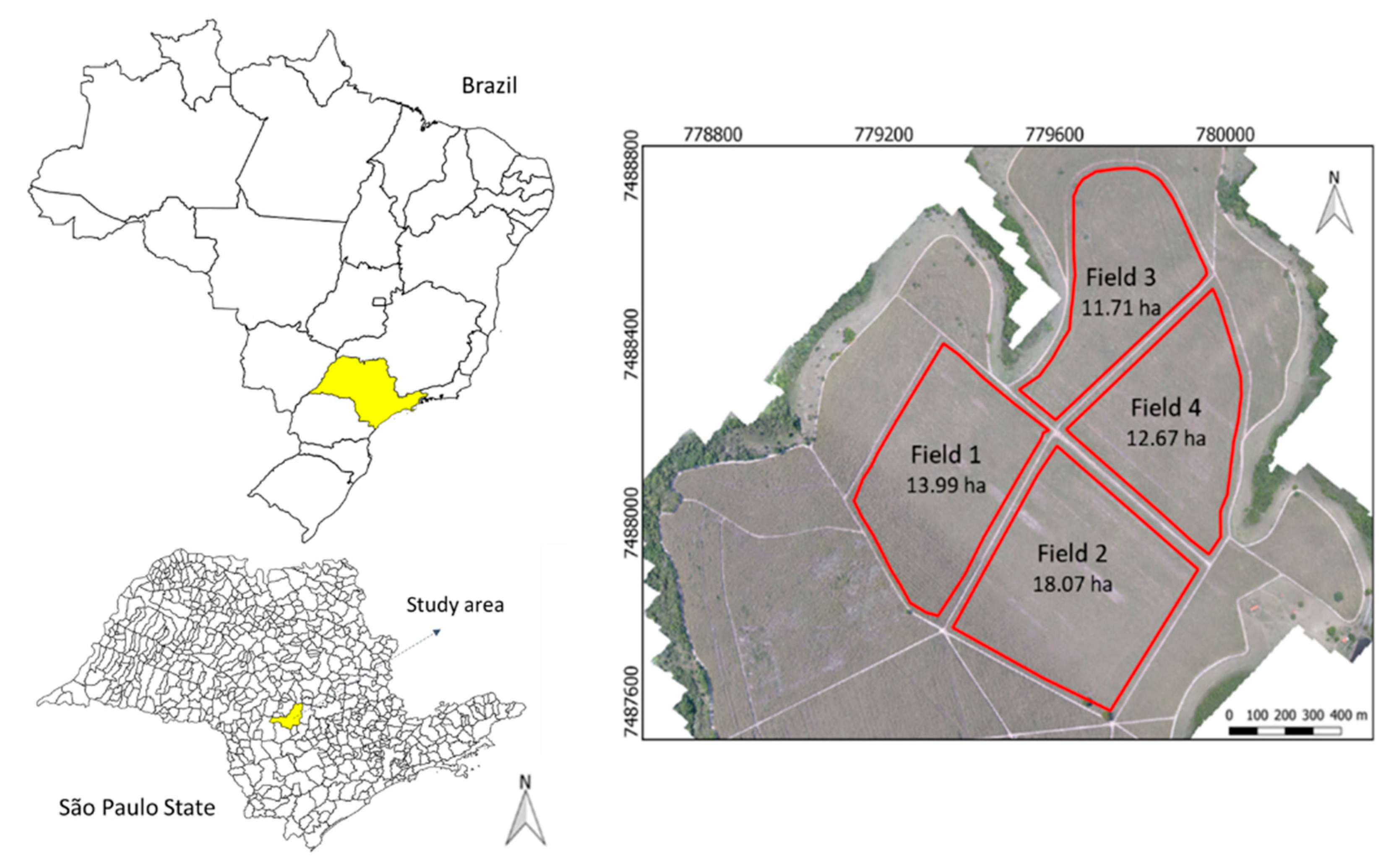
2.1. Study Site
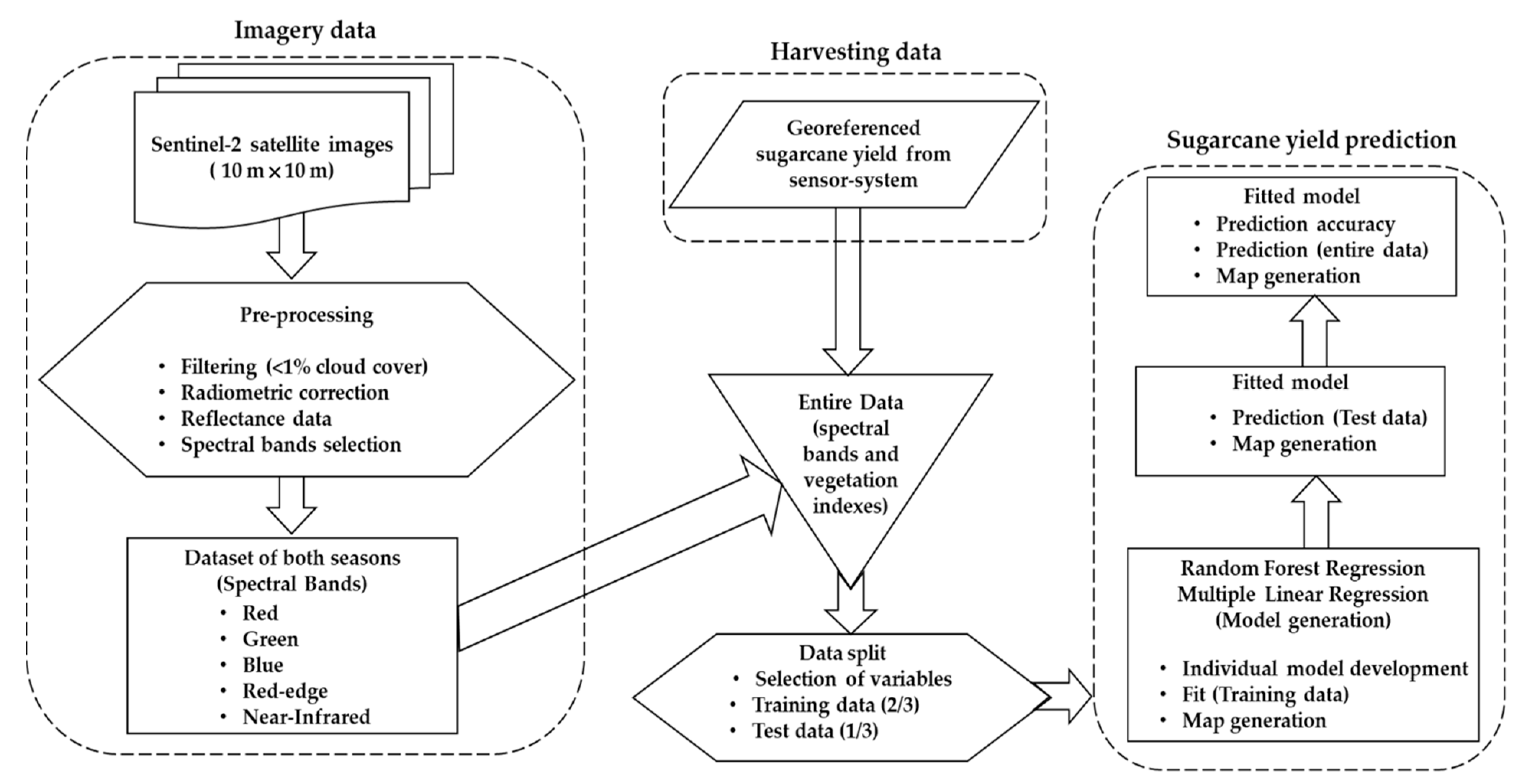
2.2. Imagery Data
2.3. Yield Data and Predictive Models
3. Results
3.1. Yield Data and Statistical Analyses
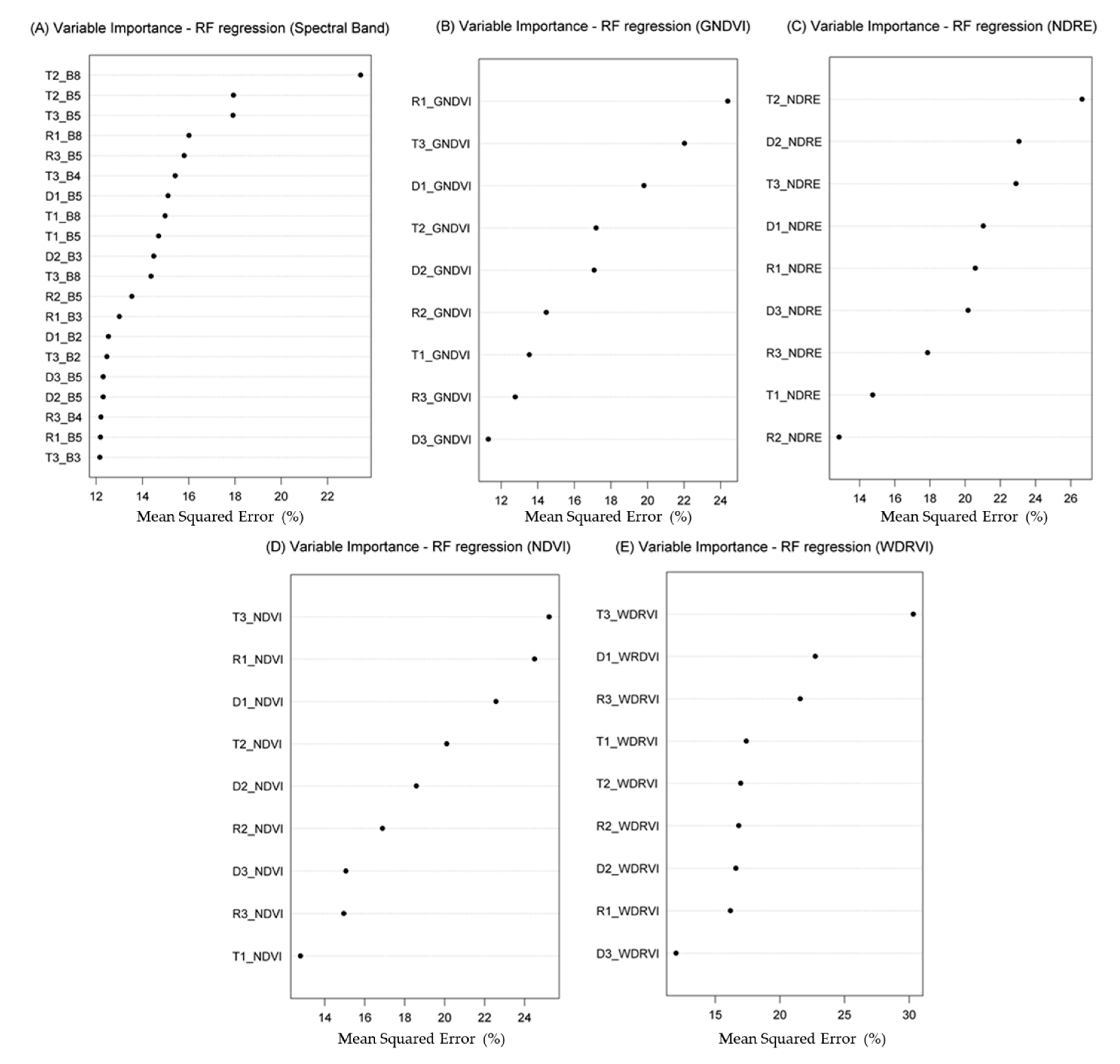
3.2. Selection of Predictor Variables
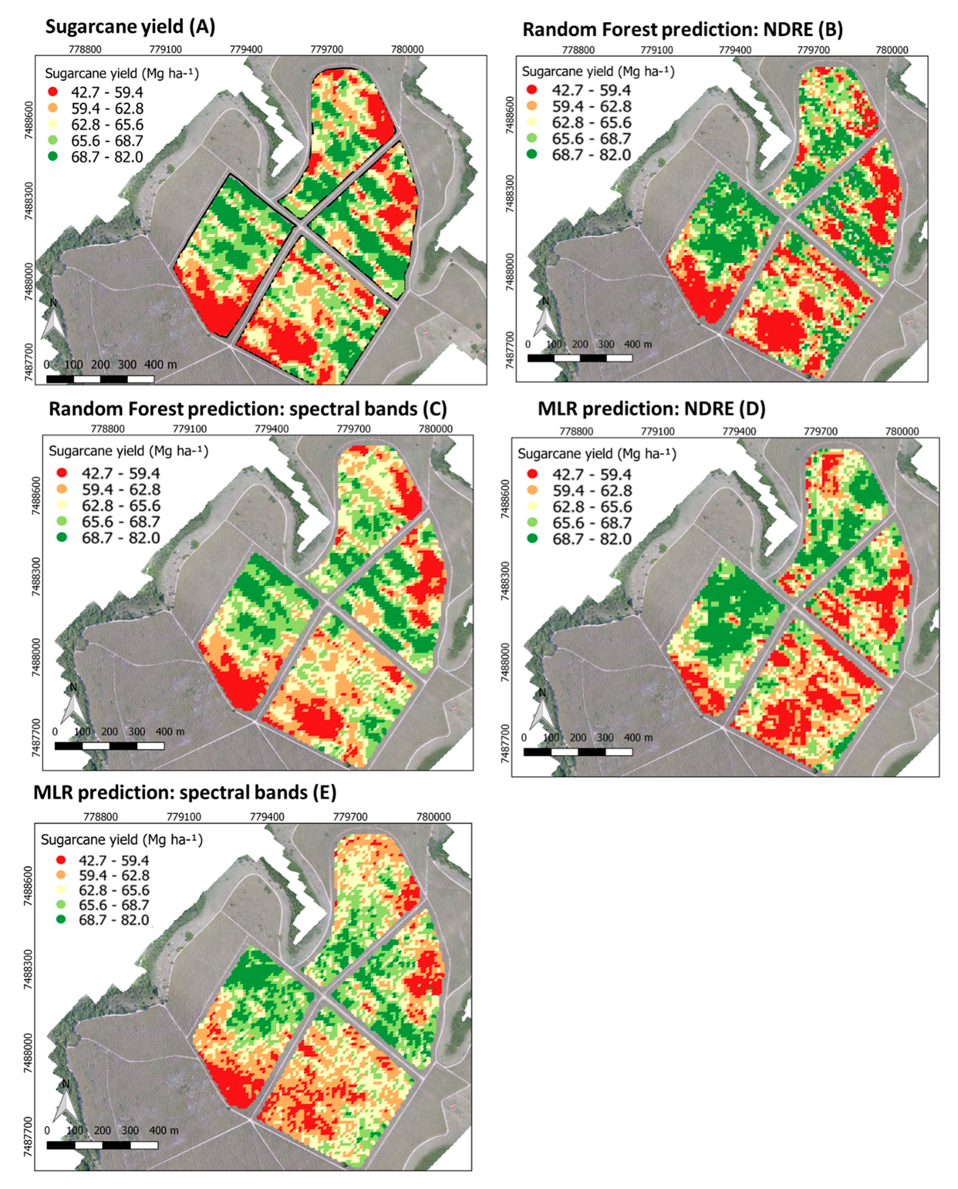
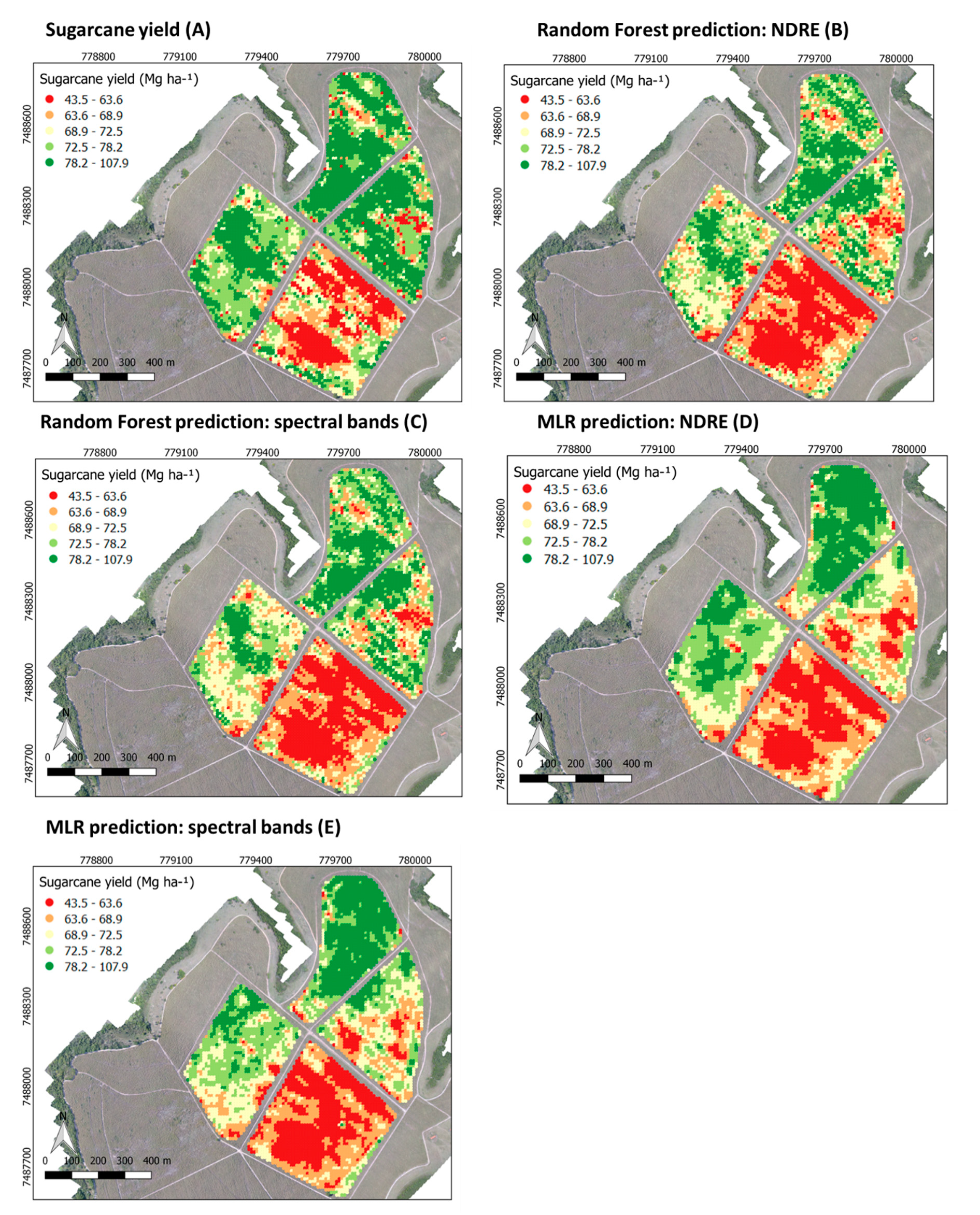
3.3. Accuracy Assessment
4. Discussion
5. Conclusions
Author Contributions
Funding
Institutional Review Board Statement
Informed Consent Statement
Acknowledgments
Conflicts of Interest
References
- Damian, J.M.; Pias, O.H.D.C.; Cherubin, M.R.; da Fonseca, A.Z.; Fornari, E.Z.; Santi, A.L. Applying the NDVI from satellite images in delimiting management zones for annual crops. Sci. Agricoia 2020, 77, e20180055. [Google Scholar] [CrossRef]
- Kayad, A.; Sozzi, M.; Gatto, S.; Marinello, F.; Pirotti, F. Monitoring within-field variability of corn yield using Sentinel-2 and machine learning techniques. Remote Sens. 2019, 11, 2873. [Google Scholar] [CrossRef]
- Baio, F.H.R.; Neves, D.C.; Campos, C.N.S.; Teodoro, P.E. Relationship between cotton productivity and variability of NDVI obtained by Landsat images. Biosci. J. 2018, 34, 197–205. [Google Scholar] [CrossRef]
- Khaliq, A.; Comba, L.; Biglia, A.; Aimonino, D.R.; Chiaberge, M.; Gay, P. Comparison of satellite and UAV-based multispectral imagery for vineyard variability assessment. Remote Sens. 2019, 11, 436. [Google Scholar] [CrossRef]
- Taghizadeh, S.; Navid, H.; Adiban, R.; Maghsodi, Y. Harvest chronological planning using a method based on satellite-derived vegetation indices and artificial neural networks. Span. J. Agric. Res. 2019, 17, 206. [Google Scholar] [CrossRef]
- Levitan, N.; Gross, B. Utilizing collocated crop growth model simulations to train agronomic satellite retrieval algorithms. Remote Sens. 2018, 10, 1968. [Google Scholar] [CrossRef]
- Cisneros, A.; Fiorio, P.; Menezes, P.; Pasqualotto, N.; Wittenberghe, V.S.; Bayma, G.; Furlan Nogueira, S. Mapping Productivity and Essential Biophysical Parameters of Cultivated Tropical Grasslands from Sentinel-2 Imagery. Agronomy 2020, 10, 711. [Google Scholar] [CrossRef]
- Sibanda, M.; Mutanga, O.; Rouget, M. Examining the potential of Sentinel-2 MSI spectral resolution in quantifying above ground biomass across different fertilizer treatments. ISPRS J. Photogramm. Remote Sens. 2015, 110, 55–65. [Google Scholar] [CrossRef]
- Lobell, D.B.; Thau, D.; Seifert, C.; Engle, E.; Little, B. A scalable satellite-based crop yield mapper. Remote Sens. Environ. 2015, 164, 324–333. [Google Scholar] [CrossRef]
- Jeffries, G.R.; Griffin, T.S.; Fleisher, D.H.; Naumova, E.N.; Koch, M.; Wardlow, B.D. Mapping sub-field maize yields in Nebraska, USA by combining remote sensing imagery, crop simulation models, and machine learning. Precis. Agric. 2020, 21, 678–694. [Google Scholar] [CrossRef]
- Schwalbert, R.A.; Amado, T.J.C.; Nieto, L.; Varela, S.; Corassa, G.M.; Horbe, T.A.N.; Rice, C.W.; Peralta, N.R.; Ciampitti, I.A. Forecasting maize yield at field scale based on high-resolution satellite imagery. Biosyst. Eng. 2018, 171, 179–192. [Google Scholar] [CrossRef]
- Lobell, D.B. The use of satellite data for crop yield gap analysis. Field Crop. Res. 2013, 143, 56–64. [Google Scholar] [CrossRef]
- Colaço, A.F.; Bramley, R. Site–Year Characteristics Have a Critical Impact on Crop Sensor Calibrations for Nitrogen Recommendations. Agron. J. 2019, 111, 2047–2059. [Google Scholar] [CrossRef]
- Bramley, R.G.V.; Ouzman, J.; Gobbett, D.L. Regional scale application of the precision agriculture thought process to promote improved fertilizer management in the Australian sugar industry. Precis. Agric. 2019, 20, 362–378. [Google Scholar] [CrossRef]
- Momin, M.A.; Grift, T.E.; Valente, D.S.; Hansen, A.C. Sugarcane yield mapping based on vehicle tracking. Precis. Agric. 2019, 20, 896–910. [Google Scholar] [CrossRef]
- Fulton, J.P.; Port, K. Precision agriculture data management. In Precision Agriculture Basics; Shannon, D.K., Clay, D.E., Kitchen, N.R., Eds.; ASA, CSSA, SSSA: Madison, WI, USA, 2018. [Google Scholar]
- Rahman, M.M.; Robson, A.J. A novel approach for sugarcane yield prediction using landsat time series imagery: A case study on bundaberg region. Adv. Remote Sens. 2016, 5, 93–102. [Google Scholar] [CrossRef]
- Mulianga, B.; Bégué, A.; Simoes, M.; Todoroff, P. Forecasting Regional Sugarcane Yield Based on Time Integral and Spatial Aggregation of MODIS NDVI. Remote Sens. 2013, 5, 2184–2199. [Google Scholar] [CrossRef]
- Bégué, A.; Lebourgeois, V.; Bappel, E.; Todoroff, P.; Pellegrino, A.; Baillarin, F.; Siegmund, B. Spatio-temporal variability of sugarcane fields and recommendations for yield forecast using NDVI. Int. J. Remote Sens. 2010, 31, 5391–5407. [Google Scholar] [CrossRef]
- Hammer, R.G.; Sentelhas, P.C.; Mariano, J.C.Q. Sugarcane yield prediction through data mining and crop simulation models. Sugar Tech. 2019, 22, 216–225. [Google Scholar] [CrossRef]
- Simões, M.D.S.; Rocha, J.V.; Lamparelli, R.A.C. Spectral variables, growth analysis and yield of sugarcane. Sci. Agric. 2005, 62, 199–207. [Google Scholar] [CrossRef]
- Abdel-Rahman, E.M.; Ahmed, F.B. The application of remote sensing techniques to sugarcane (Saccharum spp. hybrid) production: A review of the literature. Int. J. Remote Sens. 2008, 29, 3753–3767. [Google Scholar] [CrossRef]
- Lisboa, I.P.; Damian, J.M.; Cherubin, M.R.; Barros, P.P.S.; Fiorio, P.R.; Cerri, C.C.; Cerri, C.E.P. Prediction of sugarcane yield based on NDVI and concentration of leaf-tissue nutrients in fields managed with straw removal. Agronomy 2018, 8, 196. [Google Scholar] [CrossRef]
- Rahman, M.M.; Robson, A.J. Integrating Landsat-8 and Sentinel-2 Time Series Data for Yield Prediction of Sugarcane Crops at the Block Level. Remote Sens. 2020, 12, 1313. [Google Scholar] [CrossRef]
- Abdel-Rahman, E.M.; Ahmed, F.B.; Riyad, I. Random forest regression for sugarcane yield prediction based on Landsat TM derived spectral parameters. In Sugarcane: Production, Cultivation and Uses; Nova Science Publishers Inc.: Hauppauge, NY, USA, 2012; Chapter 10. [Google Scholar]
- Hunt, M.L.; Blackburn, G.A.; Carrasco, L.; Redhead, J.W.; Rowland, C.S. High resolution wheat yield mapping using Sentinel-2. Remote Sens. Environ. 2019, 233, 111410. [Google Scholar] [CrossRef]
- Jeong, J.H.; Resop, J.P.; Mueller, N.D.; Fleisher, D.H.; Yun, K.; Butler, E.E.; Timlin, D.J.; Shim, K.M.; Gerber, J.S.; Reddy, V.R.; et al. Random forests for global and regional crop yield predictions. PLoS ONE 2016, 11, e0156571. [Google Scholar] [CrossRef]
- Hochachka, W.M.; Caruana, R.; Fink, D.; Munson, A.; Riedewald, D.; Sorokina, D.; Kelling, S. Data-mining discovery of pattern and process in ecological systems. J. Wildl. Manag. 2007, 71, 2427–2437. [Google Scholar] [CrossRef]
- Yuan, H.; Yang, G.; Li, C.; Wang, Y.; Liu, J.; Yu, H.; Feng, H.; Xu, B.; Zhao, X.; Yang, X. Retrieving soybean leaf area index from unmanned aerial vehicle hyperspectral remote sensing: Analysis of RF, ANN, and SVM regression models. Remote Sens. 2017, 9, 309. [Google Scholar] [CrossRef]
- Yue, J.; Feng, H.; Yang, G.; Li, Z. A comparison of regression techniques for estimation of above-ground winter wheat biomass using near-surface spectroscopy. Remote Sens. 2018, 10, 66. [Google Scholar] [CrossRef]
- Han, L.; Yang, G.; Dai, H.; Xu, B.; Yang, H.; Feng, H.; Li, Z.; Yang, X. Modeling maize above-ground biomass based on machine learning approaches using UAV remote-sensing data. Plant Methods 2019, 15, 1–19. [Google Scholar] [CrossRef]
- Schwalbert, R.A.; Amado, T.J.C.; Nieto, L.; Corassa, G.M.; Rice, C.W.; Peralta, N.R.; Schauberger, B.; Gornott, C.; Ciampitti, I.A. Mid-season county-level corn yield forecast for US Corn Belt integrating satellite imagery and weather variables. Crop Sci. 2020, 60. [Google Scholar] [CrossRef]
- EMBRAPA—Empresa Brasileira de Pesquisa Agropecuária. Sistema Brasileiro de Classificação de Solos, 3rd ed.; Empresa Brasileira de Pesquisa Agropecuária (Embrapa): Brasília, Brazil, 2013; p. 353. [Google Scholar]
- QGIS Development Team. QGIS Geographic Information System. Open Source Geospatial Foundation Project. 2018. Available online: http://qgis.osgeo.org (accessed on 10 January 2021).
- Congedo, L. Semi-Automatic Classification Plugin Documentation. Release 2016, 4, 29. [Google Scholar] [CrossRef]
- Chavez, P., Jr. Image-Based Atmospheric Corrections—Revisited and Improved. Photogramm. Eng. Remote Sens. 1996, 62, 1025–1036. [Google Scholar]
- Rouse, J.W.; Haas, R.H.; Schell, J.A.; Deering, D.W. Monitoring vegetation systems in the great plains with ERTS. In Proceedings of the Earth Resources Technology Satellite—1 Symposium, Washington, DC, USA, 10–14 December 1974; pp. 309–317. [Google Scholar]
- Barnes, E.M.; Clarke, T.R.; Richards, S.E.; Colaizzi, P.D.; Haberland, J.; Kostrzewski, M.; Waller, P.; Choi, C.; Riley, E.; Thompson, T.; et al. Coincident detection of crop water stress, nitrogen status and canopy density using ground-based multispectral data. In Proceedings of the 5th International Conference on Precision Agriculture, Bloomington, MN, USA, 16–19 July 2000. [Google Scholar]
- Gitelson, A.A.; Kaufman, Y.J.; Merzlyak, M.N. Use of a green channel in remote sensing of global vegetation from EOS- MODIS. Remote Sens. Environ. 1996, 58, 289–298. [Google Scholar] [CrossRef]
- Gitelson, A.A. Wide Dynamic Range Vegetation Index for Remote Quantification of Crop Biophysical Characteristics. J. Plant Physiol. 2004, 161, 165–173. [Google Scholar] [CrossRef]
- Abrahão, S.A.; Pinto, F.D.A.D.C.; Queiroz, D.M.D.; Santos, N.T.; Gleriani, J.M.; Alves, E.A. Índices de vegetação de base espectral para discriminar doses de nitrogênio em capim-tanzânia. Rev. Bras. Zootec. 2009, 38, 1637–1644. [Google Scholar] [CrossRef][Green Version]
- Maresma, Á.; Ariza, M.; Martínez, E.; Lloveras, J.; Martínez-Casasnovas, J.A. Analysis of Vegetation Indices to Determine Nitrogen Application and Yield Prediction in Maize (Zea mays L.) from a Standard UAV Service. Remote Sens. 2018, 10, 368. [Google Scholar] [CrossRef]
- Matsuoka, S.; Stolf, R. Sugarcane tillering and ratooning: Key factors for a profitable cropping. In Sugarcane: Production, Cultivation and Uses; Gonçalves, J.F., Correia, K.D., Eds.; Nova Science Publishers: New York, NY, USA, 2012; Volume 5, pp. 137–157. [Google Scholar]
- Maldaner, L.F.; Molin, J.P. Data processing within rows for sugarcane yield mapping. Sci. Agric. 2020, 77, e20180391. [Google Scholar] [CrossRef]
- Minasny, B.; Mcbratney, A.B.; Whelan, B.M. VESPER Version 1.62; Australian Centre for Precision Agriculture, McMillan Building A05, The University of Sydney: Sydney, Australia, 2005. [Google Scholar]
- R Core Team. R: A Language and Environment for Statistical Computing; R Foundation for Statistical Computing: Vienna, Austria, 2018. [Google Scholar]
- Liaw, A.; Wiener, M. Classification and Regression by randomForest. R News 2020, 2, 18–22. [Google Scholar]
- Tracy, T.; Fu, Y.; Roy, I.; Jonas, E.; Glendenning, P. Towards Machine Learning on the Automata Processor. In High Performance Computing; Kunkel, J., Balaji, P., Dongarra, J., Eds.; Springer: Cham, Switzerland, 2016; Volume 9697, pp. 200–218. [Google Scholar] [CrossRef]
- Ripley, B.D. Spatial Statistics; John Wiley Sons: New York, NY, USA, 1981; Chapter 3. [Google Scholar]
- Li, W.; Jiang, J.; Guo, T.; Zhou, M.; Tang, Y.; Wang, Y.; Zhang, Y.; Cheng, T.; Zhu, Y.; Cao, W.; et al. Generating Red-Edge Images at 3 M Spatial Resolution by Fusing Sentinel-2 and Planet Satellite Products. Remote Sens. 2019, 11, 1422. [Google Scholar] [CrossRef]
- Cui, Z.; Kerekes, J.P. Potential of Red Edge Spectral Bands in Future Landsat Satellites on Agroecosystem Canopy Green Leaf Area Index Retrieval. Remote Sens. 2018, 10, 1458. [Google Scholar] [CrossRef]
- Sun, Y.; Qin, Q.; Ren, H.; Zhang, T.; Chen, S. Red-Edge Band Vegetation Indices for Leaf Area Index Estimation from Sentinel-2/MSI Imagery. IEEE Trans. Geosci. Remote Sens. 2019, 58, 826–840. [Google Scholar] [CrossRef]
- Wei, M.C.F.; Maldaner, L.F.; Ottoni, P.M.N.; Molin, J.P. Carrot Yield Mapping: A Precision Agriculture Approach Based on Machine Learning. Artif. Intell. 2020, 1, 229–241. [Google Scholar] [CrossRef]
- Venancio, L.P.; Filgueiras, R.; Cunha, F.F.D.; Silva, F.C.S.D.; Santos, R.A.D.; Mantovani, E.C. Mapping of corn phenological stages using NDVI from OLI and MODIS sensors. Semin. Ciênc. Agrar. 2020, 41, 1517–1534. [Google Scholar] [CrossRef]
- Morel, J.; Bégué, A.; Todoroff, P.; Martiné, J.F.; Lebourgeois, V.; Petit, M. Coupling a sugarcane crop model with the remotely sensed time series of fIPAR to optimise the yield estimation. Eur. J. Agron. 2014, 61, 60–68. [Google Scholar] [CrossRef]
- Dubey, S.K.; Gavli, A.S.; Yadav, S.K.; Sehgal, S.; Ray, S.S. Remote Sensing-Based Yield Forecasting for Sugarcane (Saccharum officinarum L.) Crop in India. J. Indian Soc. Remote Sens. 2018, 46, 1823–1833. [Google Scholar] [CrossRef]
- Zhao, D.; Gordon, V.S.; Comstock, J.C.; Glynn, N.C.; Johnson, R.M. Assessment of Sugarcane Yield Potential across Large Numbers of Genotypes using Canopy Reflectance Measurements. Crop Sci. 2016, 56, 1747–1759. [Google Scholar] [CrossRef]


| Spectral Bands | Central Wavelength (nm) | Resolution | ||
|---|---|---|---|---|
| Spatial (m) | Temporal (Days) | Radiometric (Bits) | ||
| B2 Blue | 490 | 10 | 5 | 12 |
| B3 Green | 560 | |||
| B4 Red | 665 | |||
| B8 NIR | 842 | |||
| B5 Red-Edge | 705 | 20 | ||
| Vegetation Index | Equation | Authors |
|---|---|---|
| Normalized Difference Vegetation Index | NDVI = (NIR − Red)/(NIR + Red) | Rouse et al. [37] |
| Normalized Difference Red-Edge Index | NDRE = (NIR − Red-edge)/(NIR + Red-edge) | Barnes et al. [38] |
| Green Normalized Difference Vegetation Index | GNDVI = (NIR − Green)/(NIR + Green) | Gitelson et al. [39] |
| Wide Dynamic Range Vegetation Index | WDRVI = (a × NIR − Red)/(a × NIR + Red) | Gitelson [40] |
| ID | DAC | Orbital Image Dates in 2018 (Month/Day) | Orbital Image Dates in 2019 (Month/Day) | Phenological Stage |
|---|---|---|---|---|
| I1 | 30 | NA | NA | Initial |
| I2 | 60 | NA | NA | Initial |
| T1 | 90 | 02/04, 02/09, 02/24 | 02/09 | Tillering |
| T2 | 120 | 03/06, 03/11, 03/16, 03/21 | 03/06, 03/26, 03/31 | Tillering |
| T3 | 150 | 04/05, 04/20, 04/25, 04/30 | 04/20, 04/25 | Tillering |
| D1 | 180 | 05/20, 05/30 | 05/05, 05/30 | Development |
| D2 | 210 | 06/19, 06/29 | 06/09, 06/14, 06/24, 06/29 | Development |
| D3 | 240 | 07/04, 07/09, 07/14, 07/19, 07/24, 07/29 | 07/09, 07/14, 07/24 | Development |
| R1 | 270 | 08/13, 08/18, 08/23, 08/28 | 08/08, 08/18, 08/23, 08/28 | Ripening |
| R2 | 300 | 09/07, 09/22 | 09/07, 09/12, 09/17 | Ripening |
| R3 | 330 | 10/12, 10/22 | 10/02, 10/12, 10/17 | Ripening |
| M | 360 | NA | NA | Maturation |
| Season | Dataset | n | Minimum | Median | Mean | Maximum | SD | CV (%) |
|---|---|---|---|---|---|---|---|---|
| Mg ha−1 | ||||||||
| 2018/2019 | Original | 53,759 | 0.86 | 70.85 | 71.20 | 501.23 | 23.53 | 33.04 |
| 2018/2019 | Filtered | 16,202 | 36.03 | 64.43 | 64.31 | 86.35 | 7.06 | 10.98 |
| 2019/2020 | Original | 67,716 | 10.39 | 72.52 | 112.90 | 498.21 | 81.96 | 72.60 |
| 2019/2020 | Filtered | 28,247 | 42.74 | 65.82 | 70.92 | 107.90 | 9.55 | 13.47 |
| Season | n | Model | Range (m) | Sill | Nugget | RMSE (Mg ha−1) | Calc. Grid (Samples ha−1) |
|---|---|---|---|---|---|---|---|
| 2018/2019 | 5616 | Exponential | 42.04 | 33.79 | 12.95 | 0.53 | 23 |
| 2019/2020 | 5686 | Exponential | 49.30 | 23.54 | 5.19 | 1.41 | 16 |
| Random Forest | Multiple Linear Regression | ||||||
|---|---|---|---|---|---|---|---|
| Variables | Dataset | RMSE | R2 | MAE | RMSE | R2 | MAE |
| Spectral bands | Training | 1.95 | 0.96 | 1.42 | 6.10 | 0.48 | 4.73 |
| Testing | 4.63 | 0.70 | 3.46 | 6.11 | 0.47 | 4.67 | |
| Entire | 3.13 | 0.87 | 2.11 | 6.10 | 0.47 | 4.71 | |
| GNDVI | Training | 2.44 | 0.93 | 1.83 | 6.35 | 0.44 | 4.92 |
| Testing | 5.47 | 0.57 | 4.21 | 6.14 | 0.46 | 4.79 | |
| Entire | 3.76 | 0.81 | 2.64 | 6.28 | 0.44 | 4.87 | |
| NDRE | Training | 2.39 | 0.94 | 1.79 | 6.36 | 0.43 | 4.93 |
| Testing | 5.30 | 0.60 | 4.06 | 6.18 | 0.45 | 4.82 | |
| Entire | 3.65 | 0.82 | 2.56 | 6.30 | 0.44 | 4.89 | |
| NDVI | Training | 2.42 | 0.93 | 1.81 | 6.39 | 0.43 | 4.93 |
| Testing | 5.39 | 0.58 | 4.18 | 6.21 | 0.45 | 4.83 | |
| Entire | 3.71 | 0.81 | 2.62 | 6.33 | 0.43 | 4.90 | |
| WDRVI | Training | 2.41 | 0.94 | 1.81 | 6.36 | 0.43 | 4.93 |
| Testing | 5.43 | 0.58 | 4.20 | 6.18 | 0.45 | 4.81 | |
| Entire | 3.73 | 0.81 | 2.62 | 6.30 | 0.44 | 4.89 | |
Publisher’s Note: MDPI stays neutral with regard to jurisdictional claims in published maps and institutional affiliations. |
© 2021 by the authors. Licensee MDPI, Basel, Switzerland. This article is an open access article distributed under the terms and conditions of the Creative Commons Attribution (CC BY) license (http://creativecommons.org/licenses/by/4.0/).
Share and Cite
Canata, T.F.; Wei, M.C.F.; Maldaner, L.F.; Molin, J.P. Sugarcane Yield Mapping Using High-Resolution Imagery Data and Machine Learning Technique. Remote Sens. 2021, 13, 232. https://doi.org/10.3390/rs13020232
Canata TF, Wei MCF, Maldaner LF, Molin JP. Sugarcane Yield Mapping Using High-Resolution Imagery Data and Machine Learning Technique. Remote Sensing. 2021; 13(2):232. https://doi.org/10.3390/rs13020232
Chicago/Turabian StyleCanata, Tatiana Fernanda, Marcelo Chan Fu Wei, Leonardo Felipe Maldaner, and José Paulo Molin. 2021. "Sugarcane Yield Mapping Using High-Resolution Imagery Data and Machine Learning Technique" Remote Sensing 13, no. 2: 232. https://doi.org/10.3390/rs13020232
APA StyleCanata, T. F., Wei, M. C. F., Maldaner, L. F., & Molin, J. P. (2021). Sugarcane Yield Mapping Using High-Resolution Imagery Data and Machine Learning Technique. Remote Sensing, 13(2), 232. https://doi.org/10.3390/rs13020232