Abstract
Among various ways to eliminate the multipath effect in high-precision global navigation satellite system positioning, the multipath hemispherical map (MHM) is a typical multipath correction method based on spatial domain repeatability, which is suitable for not only static environments, but also some dynamic carriers, such as ships and aircraft. So, it has notable advantages and is widely used. The MHM method divides the sky into grids according to the azimuth and elevation angles of satellite, and calculates the average of the residuals within the grid points as its multipath calibration value. It is easy to implement, but it will inevitably lead to excessive or insufficient multipath correction in the grid. The trend surface analysis-based multipath hemispherical map (T-MHM) method makes up for this deficiency by performing trend surface analysis on the multipath spatial changes within the grid points. However, the effectiveness of T-MHM is limited and less capable of resisting noise interference due to the multicollinearity between the independent variables caused by the special spatial distribution of multipath sampling and the overfitting problem caused by ignoring the multipath anisotropy. Thus, we proposed an improved multipath elimination method named AT-MHM (advanced trend surface analysis-based multipath hemispherical model), which cautiously judges the occurrence of the above problems and gives corresponding solutions. This was extended to double-difference mode, which expands the scope of application. The performance of AT-MHM in GPS pseudorange multipath mitigation was verified on geodetic receiver and low-cost receiver in a strong multipath environment with high occlusion.
1. Introduction
Multipath error is one of the key unresolved errors in global navigation satellite system (GNSS) positioning, as it is difficult to parameterize and cannot be eliminated by differential technology. At present, the methods to suppress multipath error are mainly divided into hardware-based and software-based. The hardware-based method includes improvements of the antenna and receiver. The antenna improvement methods mainly include the patch elements placed on choke rings [1], the multipath estimating delay-locked loop [2,3] and a “narrow correlator” delay-locked loop [4], which can only partially eliminate multipath error. Antenna-related improvements also include array antennas [5,6,7,8,9,10] and dual-polarized antenna techniques [11,12,13]. The above methods effectively suppress the multipath effect, but increase the hardware cost.
There are four types of data processing methods. The first category makes use of the correlation between the carrier to noise power density ratio (C/N0) and multipath error to reduce the error of the multipath positioning results according to the observed value of C/N0 [14]. However, the attenuation of the direct signal may lead to the decrease in C/N0, and the reflected signal strength of glass, metal, and wet surfaces may be equivalent to that of the direct signal [15]. The second category is based on a time series analysis. Zhong et al., Satirapod et al., and others used the Vondrak filter, empirical mode decomposition (EMD), and wavelet analysis to construct multipath mitigation models [16,17,18]. This type of method separates the multipath error from the residual time series and performs post-processing corrections on the same observation sequence, which is inconvenient to realize the real-time calculation and correction of the multipath effect.
The third category method is based on the repetitive period of satellite constellation distribution in time domain, including sidereal filtering (SF) [19], modified sidereal filtering (MSF) [20,21,22,23] and Advanced Sidereal filtering (ASF) [24,25,26,27]. This type of method calculates the precise repeat periods of satellite orbits. In addition, it is only suitable for static environments and is difficult to extend to dynamic environments. The fourth category is modeling based on multipath spatial domain repeatability. As long as the primary multipath environment between the antenna and its carrier does not change, the multipath error is only related to the elevation and azimuth angle of the satellite, and irrelevant to which satellite. Based on this feature, the application of multipath mitigation can be extended from static scenes to dynamic scenes (such as ships and aircrafts) with an unchanged primary multipath environment.
There are several ideas in multipath modeling based on spatial domain repeatability. Cohen constructed a 12th spherical harmonic model to fit the multipath error [28]. This method is equivalent to the revolution of a 30° × 30° grid size. However, to meet the positioning accuracy requirements, it is typically necessary to use a fine mesh (such as 1° × 1°). Due to the high computational complexity of high-order spherical harmonic model, some studies divided the sky into grids according to the equal angle interval [29] or equal area [30] and then calculated the mean value of the residual error within the grid points as its multipath.
This type of method is simple to implement and has low complexity; however, the spatial distribution of the multipath inside the grid is ignored, which leads to a better correction effect for a low-frequency multipath and limited modification for a high-frequency multipath [29]. To solve this problem, Wang et al. established a trend surface analysis-based multipath hemispherical model (T-MHM), which uses the trend surface polynomials of different orders to simulate the variation of multipaths in grids and to realize the reduction in both low-frequency and high-frequency multipaths [31]. This method provides in-depth modeling within MHM grids. By combining the statistical method of spatial analysis with the time–space repeatability of multipaths, this method can be more capable for a complex multipath environment.
However, some weaknesses that affect the trend surface analysis should be investigated and further remedied. First, when there is only one satellite trajectory in the grid, the multicollinearity problem exists among the regression independent parameters, which leads to the singularity of the equation. The least squares solution obtained in this case may be close to ill-conditioned; thus, it is necessary to be cautious in the substantial interpretation of the multipath spatial pattern [32]. Second, multipath errors are closely related to the environment. Therefore, the multipath errors may exhibit strong spatial anisotropy even within a certain grid, which is modeled by a few skew paths of satellites in T-MHM fitting, where the elevation and azimuth parameters are always given the same weights. Such a treatment may fit part of the noise or other interference, causing overfitting.
Based on the above analysis, an improved method named advanced trend surface analysis-based multipath hemispherical model (AT-MHM) was proposed to remedy the weakness in the application of T-MHM and enhance the anti-interference capability. In order to be adaptable for more general applications, AT-MHM adopts the “Zero Mean” method to obtain single-difference multipath values through double-difference residual conversion [33]. We verified the performance of pseudorange multipath correction for the geodetic receiver in a strong multipath environment and discussed the feasibility of multipath correction for low-cost equipment.
In the following sections, we first introduce the modeling process of AT-MHM. Then, the key factors affecting the effectiveness of the trend surface analysis results are discussed, detailed data examples and analysis are listed, and AT-MHM solutions are given for these drawbacks. In Section 3 and Section 4, the experimental settings and data processing results of both geodetic receiver and low-cost receiver are introduced and discussed. The last section concludes with a summary.
2. Methodology of AT-MHM
AT-MHM is established on the basis of the T-MHM method, and its modeling process is as shown in Figure 1. First, we solve the baseline solution and extract the multipath error from the double difference residuals as the input for the next modeling step. Second, we define the grids for the proposed model by azimuth and elevation angles and conduct the advanced trend surface analysis for all converted single-difference observable residuals residing in this lattice, which will be described in detail in Section 2.3. Finally, we choose the appropriate model based on the statistical criteria and store the proper set of multipath correction coefficients or the average value of the multipath. The steps shown in the blue box in the Figure 1 are the improvements in AT-MHM compared with T-MHM.
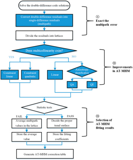
Figure 1.
Flow chart of advanced trend surface analysis-based multipath hemispherical model (AT-MHM) construction.
All the above steps are programmed in the software RPAD (realtime position and attitude determination) independently developed by our team. While implementing multipath correction using the AT-MHM, the required correction table will be loaded. For an epoch, we first calculate the satellite’s azimuth and elevation, query the corresponding grid points of the correction table to obtain the trend surface coefficients, and then substitute the satellite angle to calculate the multipath estimation value, and finally deduct it from the double-difference observation minus calculation value. In the following sections, we mainly introduce the details of key modeling steps of AT-MHM.
2.1. Extract the Multipath Error from Short Baseline Double-Difference Residuals
Let be the GPS L1 pseudorange observations of satellite i, j received by receiver U, and be the observations of satellite i, j received by receiver R. The single-difference observation equation can be expressed as:
Then, the double-difference observation equation can be expressed as:
where is the double-difference satellite-receiver distance corresponding to receiver U and receiver R, and satellite i and satellite j. Short baseline double-difference effectively eliminates the atmospheric error, ionosphere, orbital errors, and the clock offset of both the satellite and receiver. For an epoch, the position parameters were estimated by least square algorithm. When the coordinates of the rover and the base station are known or have a reliable solution, in the equation can be determined and fixed. Then, the residual can be considered mainly as the double-difference multipath error plus the observation noise. As the AT-MHM method is also based on the spatial repeatability of the multipath, it is necessary to establish the relationship between the multipath and the satellite elevation and azimuth. Therefore, the double-difference multipath value cannot be used directly, and it must be converted into a single-difference residual value.
Here, we adopt the “zero mean” assumption [24,33] and express the double-difference multipath value as the product of a matrix and single-difference seen as Equation (4).
Assuming that n shared satellites were received by two stations at this epoch, the satellite j with the highest elevation angle was selected as the reference satellite. Then, as calculated by the reciprocal of the elevation angle of satellite i, and let. The single-difference multipath value can be obtained by matrix inversion. The method of converting double-difference to single-difference was originally used to study the atmospheric water component, and later Zhong et al. used it to model the filtering residuals of the sidereal day.
2.2. Overview of the T-MHM Method
The mathematical equations used to calculate the trend surface include polynomial functions and Fourier series. T-MHM utilizes commonly used polynomial functions, which are expressed as
Equations (5)–(7) are the formulas for the linear, quadratic, and cubic trend surfaces, respectively, where represents the multipath estimation value at the residual point with azimuth angle and elevation angle , and represent the integer index of the sky grid . For example, when the model utilizes ° ×° resolution, there are a total of grids, and the grid contains all residual points of satellite azimuth falling in interval and elevation falling in interval .
The trend surface formula of the T-MHM method can be expressed in matrix form, as shown in Equations (8) and (9).
where n is the total number of sample points within the grid, is the multipath error (converted single-difference residual) assigned to the grid , r represents the fitting order of the trend surface model, and p represents the number of trend surface coefficients. The conventional least squares unbiased estimation of trend surface coefficients can be obtained using Equation (10). Then, through the goodness of fit test and significance tests, a suitable trend surface was selected from linear, quadratic, and cubic trend surface fittings. When the goodness of fit test result is less than 0.3 or significance test fails, that fitting result will not be adopted. If both the lower and higher order trend surface fitting can satisfy the conditions, successive significance test is essential to confirm whether progressively higher order is meaningful [34]. In two cases, the average of residuals will be used as the multipath correction value. One case is that all the fitting results fail the statistical tests, and the other is when the number of residual points in the grid is less than a certain amount, for example, we set a minimum of 24 by trial. The related equations of the goodness of fit test and significance tests are given in Table 1.

Table 1.
Statistical tests of trend surface analysis.
2.3. Improvements in AT-MHM
The T-MHM method adopts the method of fitting the trend surface and considers the spatial position relationship between points and the spatial trend change of the multipath, which has been verified to be effective for multipath mitigation in both low and high frequency bands. However, in practical application, we found that the trend surface fitting formula may not adapt properly to some situations. In this section, the constraint methods and improvements adopted by AT-MHM are introduced.
2.3.1. Identification and Solution of the Multicollinearity Problem
To meet the requirements of positioning accuracy, we typically divided the sky into grids of appropriate scale when establishing the multipath correction model. Figure 2a shows the multipath skymap obtained from static observations. We see that, even if many intersection points of satellite orbits exist, there are many grids (1° × 1° resolution) with only one track passing through (Figure 2b). As the trajectory is approximate to a straight line, the parameters are highly linear correlated in numerical value, resulting in the ill-conditioned fitting trend surface, seen as Figure 2c. The trend of the fitted plane in the direction orthogonal to the trajectory is nearly singular, which leads to a large uncertainty of trend in this direction and weak resistance to noise perturbation. Even the result of this trend surface fitting has a high goodness of fit as the small disturbances in data space due to system noises tend to cause large fluctuations in the results of model space. Hence, trend surface analysis should be cautiously performed to interpret the spatial pattern of multipaths of a single-trajectory grid.
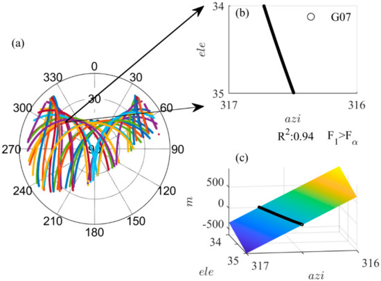
Figure 2.
Spatial distribution of the multipath value in a single-trajectory grid (35, 317). (a) Sky plot of satellite trajectories. (b) Projection of the multipath value in grid (35, 317) on the plane of elevation and azimuth. (c) trend surface analysis-based multipath hemispherical model (T-MHM) linear trend surface fitting of grid (35, 317).
The methods to judge and eliminate multicollinearity include increasing the sample size, eliminating the collinearity parameters, and ridge regression. Boots et al. and Wheeler et al. utilized the linear combination of eigenvectors of other parameters to eliminate one of the collinear parameters [32,35]. Similarly, AT-MHM adopts the constrained least squares fitting method, as shown in Equation (11), in which the parameters and can be obtained by linear fit to and . If the (seen in Table 1) of equation is greater than 0.9, then it is almost certain that this grid satisfies the case of multicollinearity. This is also a fast way to judge this situation without storing satellite numbers.
We replace one of the parameters by the linear combination fitted in Equation (11). The constrained variable matrix is shown in Equation (12). Then, the constrained estimation of trend surface coefficients is obtained with Equation (13).
Finally, the estimated value is calculated for the statistical test of the current model, shown as Equation (14), where the N is the observed variable matrix in Equation (9).
To show the difference between the constrained least squares fitting and the original T-MHM method, the grid (35, 317) is still taken as an example. The statistical test results of the linear and quadratic fitting trend surface of AT-MHM are shown in Table 2. The constrained linear and quadratic fitting results both passed the significance test, in which the goodness of fit of linear model relative to T-MHM is reduced a little. The two fitting surfaces are displayed in Figure 3, where (a) and (c) are the linear and quadratic trend surface under constraints, respectively.
Table 2.
Statistical tests of constrained linear and quadratic fitting of the trend surfaces of grid (35, 317).
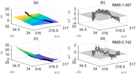
Figure 3.
Constrained trend surface fitting results of grid (35, 317). (a) Linear trend surface fitting with constraints. (b) Residual plot of target multipath value minus constrained linear fitting trend surface fitting. (c) Quadratic trend surface fitting with constraints. (d) Residual plot of target multipath value minus constrained quadratic trend surface fitting. X, Y-axis unit: degree, Z-axis unit: meter.
Compared with Figure 2c, we see that the fitting surfaces of the constrained method are quite different in areas lacking data (Figure 3a,c). Then, we take the multipath errors in the same grid of the next day as the target, written as , and estimate the correction value from two models, which is expressed as . The differences between and are shown in Figure 3b,d. From the results of the statistical test and actual mitigation, the goodness of fit and correction effect of quadratic trend surface fitting were much better. According to the conclusion of Wang et al. [31], it is unnecessary to consider cubic trend surface fitting for the grid points with a resolution of.
2.3.2. Identification and Solution of the Anisotropic Problem
The nature of a multipath is closely related to the environment; therefore, the variation characteristics of the multipath error in the azimuth and elevation parameters are likely different to reflect the spatial anisotropy. In the expression of the trend surface model, the linear term contributes to the trend of the data, while quadratic or high-order terms fit local non-linear variations. In the application of multipath correction, proper quadratic or high-order terms in the elevation and azimuth directions, respectively, should be chosen to model multipath anisotropy and to avoid over fitting. Then, by analyzing the co-correlation among the multipath, elevation, and azimuth, AT-MHM determines which parameter in this grid has a greater impact on the multipath variation. The Pearson correlation coefficient (PCC) is adopted as the criterion, and its calculation is shown as Equation (15) [36].
where n is the number of sample points within the grid; are the mean values and the standard deviations, respectively, of A, B. When the absolute value of PCC is 0.8–1.0, the two variables are highly correlated, 0.6–0.8 are a strong correlation, 0.4–0.6 are a moderate correlation, 0.2–0.4 are a weak correlation, and finally 0.0–0.2 are an extremely weak correlation or no correlation. When considering the quadratic trend surface fitting, T-MHM uses the same highest power for parameters and , as shown in Equation (6). While AT-MHM adopts quadratic term for the parameter which has greater correlation with multipath variation, and only linear term is used for the other parameter. Therefore, there are two quadratic trend surface fitting forms of AT-MHM, which correspond to the higher correlation between azimuth and multipath and the higher correlation between elevation and multipath, as shown in formula 16.
The above two forms are named QE and QA, respectively. Next, we use two examples to prove the necessity and effectiveness of using different forms of quadratic trend surface fitting formulas for different multipath anisotropy performance. For each example, we will fit the linear, T-MHM quadratic, QA and QE trend surfaces respectively, and compare the statistical test results and the actual multi-path correction effect of these four models.
- Case 1
The first example shows the grid type suitable for selecting the QE trend surface. The grid (30, 313) is shown in Figure 4. In order to intuitively show the variation of the multipath error in space, we use different colors in a 2D heat map to represent the value at the corresponding positions. From the color change and PCC results, the multipath error clearly varies with the elevation in this grid.
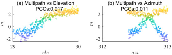
Figure 4.
The multipath error varies closely with the elevation in grid (30, 313). (a) Correlation between the elevation and multipath. (b) Correlation between the azimuth and multipath. X-axis unit: degree, Y-axis unit: meter. Pearson correlation coefficient (PCC).
We used the data of the previous day to construct linear, quadratic, QA, and QE models to correct the same grid point of the next day and to observe the change of residuals after multipath correction. The statistical test results of four models are given in Table 3. The models of the previous day all show very strong trend patterns. The goodness of fit of the quadratic, QA, and QE trend surface models are only different from the third decimal place, in which the quadratic trend surface obtained the highest score. Next, we will test the performance of these models for the next day. The results of the multipath reduction are shown in Figure 5. We first noticed that the linear trend surface and the QE trend surface achieved better correction effects followed by the QA trend surface, while the quadratic trend surface with the highest goodness of fit introduced larger errors in local areas.
Table 3.
The statistical test results of models constructed from the previous day.
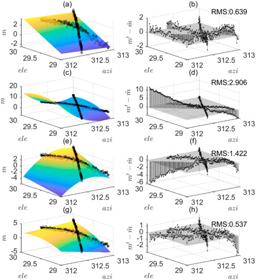
Figure 5.
The fitting and application results of four trend surface models constructed from the previous day of grid (30, 313). (a,b) The fitting surface and residual plot after multipath correction of the linear trend surface model. (c,d) The fitting surface and residual plot after multipath correction of the T-MHM quadratic trend surface model. (e,f) The fitting surface and residual plot after multipath correction of the AT-MHM QA trend surface model. (g,h) The fitting surface and residual plot after multipath correction of the AT-MHM QE trend surface model. X, Y-axis unit: degree, Z-axis unit: meter.
The satellite data in the modeling day were sometimes less than in the corrected day, which may be due to the short observation time, signal blocking, satellite orbit adjustment, and other causes. The results of the fitting surface and residual plot in Figure 5c,d show that quadratic trend surface model overestimated the areas lacking data and caused large errors. In addition, the results of the QA trend surface model also demonstrated that (Figure 5e,f). The QE model was fitted conservatively on the parameters with less influence, which not only improved the fitting performance compared with the linear trend surface but also did not appear to over-fit the results of the quadratic trend surface, thus obtaining the best correction effect (Figure 5g,h).
- Case 2
Next, the grid type suitable for selecting QA trend surface is illustrated in Figure 6. We also used the data of the previous day to construct linear, quadratic, QA, and QE models to correct the same grid points of the next day. The statistical test results of the four models are given in Table 4. The goodness of fit of the quadratic trend surface, QA, and QE also achieved almost the same results, and they all passed the successive significance test.
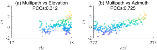
Figure 6.
The multipath error varies closely with the azimuth in grid (18, 273). (a) Correlation between the elevation and multipath. (b) Correlation between the azimuth and multipath. X-axis unit: degree, Y-axis unit: meter.
Table 4.
Statistical test results of four types of fitting trend surfaces of grid (318, 10).
The multipath reduction effects of these models for the next day are shown in Figure 7. The results of root mean square (RMS) after multipath correction show that the order of correction effectiveness was QA, QE, linear, and quadratic model. From the four fitting trend surfaces on the left (Figure 7a,c,e,g), the linear and QA trend surface better reflected the variation of the multipath value with the azimuth, while the quadratic and QE trend surfaces exhibited poor extension due to a quadratic term in the elevation parameter.
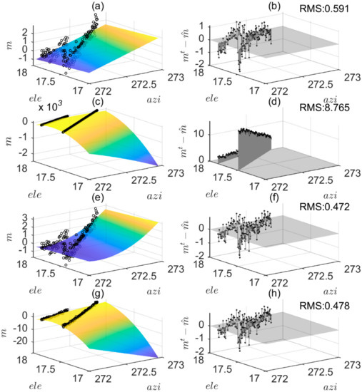
Figure 7.
The fitting and application results of the four trend surface models constructed from the previous day of grid (18,273). (a,b) The fitting surface and residual plot after multipath correction of the linear trend surface model. (c,d) The fitting surface and residual plot after multipath correction of the T-MHM quadratic trend surface model. (e,f) The fitting surface and residual plot after multipath correction of the AT-MHM QA trend surface model. (g,h) The fitting surface and residual plot after multipath correction of the AT-MHM QE trend surface model. X, Y-axis unit: degree, Z-axis unit: meter.
Both of the above examples illustrate that for a grid with obvious anisotropy, even if the statistical test was passed, the prediction of subsequent observations may be inaccurate if the high-order terms are not used properly.
3. Experiment Validations of Geodetic Receiver
A short baseline experiment was conducted from DOY (day of year) 50 to 52, 2019, every day from 5:00 to 17:00 UTC at the campus of the East China Normal University. Each day the sampling rate was 1 Hz. The rover station used a Trimble BD982 receiver and was placed on the balcony near the office window on the fourth floor of the Communication and Electronic Engineering Building (Left panel of Figure 8). Choosing such a scene can simulate the high shelter of the city environment and ensure a strong interference multipath error. The base station utilized the Continuously Operating Reference Station (CORS), as shown in right panel of Figure 8, erected on the roof of the Estuary and Coast College, approximately 56.7 m away from the rover station. The CORS station used a Trimble R9 receiver, and the sampling frequency was also 1 Hz.
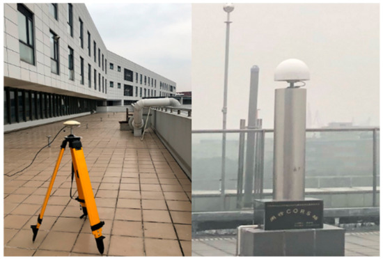
Figure 8.
Surrounding environments of the rover station and reference station.
3.1. Multipath Error Assessment of Geodetic Receiver
Before discussing general multipath modeling and correction effects, we evaluated the multipath error of the geodetic receiver in the environment shown in Figure 8. According to the workflow introduced in the theory part, we used the data of DOY 50 and took the centimeter level precision coordinate results calculated by GAMIT as the true value of the rover station, and then solved the double-difference fixed solution residual of the GPS pseudorange observables. The double-difference residuals can be considered to have eliminated the common errors, such as the ionosphere and troposphere, and are mainly composed of multipath errors and random noises.
Then, we used the “Zero Mean” method to obtain the new single-difference residual converted from the double-difference residual, which is represented by the “ZM single-difference” later. The probability density histogram is shown in the left panel of Figure 9. We can see that the mean value of the multipath error value of this experiment was near zero, distributed between −15.32 and 20.77 m, of which 98.5% of the values fell between −3 and +3 m. We drew the skymap of the ZM single-difference, as shown in the right panel of Figure 9. The azimuth angle of 90 to 210 degrees was blocked by the building, and the satellite signal could hardly be received. The larger values of the multipath were distributed in the direction of azimuth 30 to 90 degrees and 230 to 320 degrees, which were interfered with by the reflected signal from the wall.
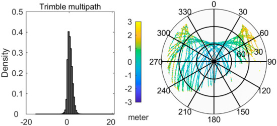
Figure 9.
The probability density histogram(left) and sky map(right) of the multipath error of day of year (DOY) 50.
3.2. Comparison of MHM, T-MHM, and AT-MHM in Double-Difference Mode for the Geodetic Receiver
Next, we performed two tests to compare the improvement effect of the pseudorange positioning accuracy of the geodetic receiver after multipath correction using MHM, T-MHM, and AT-MHM. The first test was to simulate the ideal situation where the spatial repetition rate of multipath effect can reach 100%. We utilized DOY50 modeling to correct the multipath of itself. The results show that the AT-MHM model achieved the best results in three directions, and the baseline accuracy was improved by approximately 45.98%, 58.68%, and 43.93% in the three directions of east, north, and vertical, respectively (Table 5). Compared with T-MHM, the improvement in the north was more obvious.
Table 5.
The root mean square error (RMSE) comparison between solutions of MHM, T-MHM, and AT-MHM on DOY 50. (Unit: meter).
The east direction (left panel) and north direction (right panel) of the baseline solution are shown in Figure 10. This demonstrates both the high frequency error and low frequency error, and the correction effect of MHM (blue) for the low-frequency multipath (7:00–9:00 and 16:00–17:00) was clearly better than that of the high-frequency error (10:00–11:00, 12:00–13:00, and 13:00–14:00). The results of T-MHM (green) also improve the high frequency multipath, but also brought some errors. The low frequency and high frequency multipath correction results of AT-MHM (red) are better than both MHM and T-MHM. Compared with the uncorrected solutions (gray), the improved epochs of MHM, T-MHM, and AT-MHM accounted for 70.51%, 75.31%, and 76.02% of the total epochs respectively in north direction.
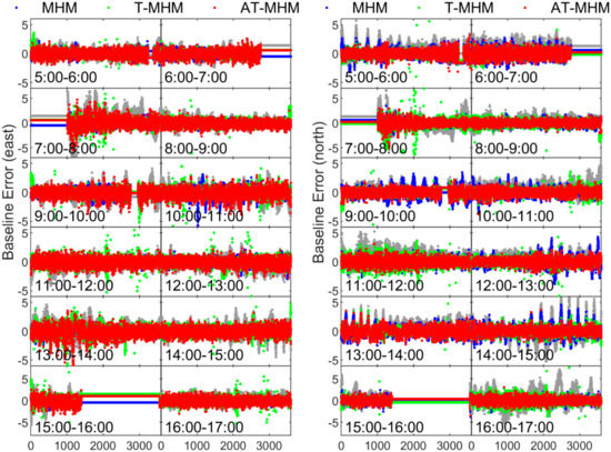
Figure 10.
The results of the east (left panel) and north (right panel) directions before and after multipath correction on DOY 50. The color gray in the figure represents the uncorrected baseline solution of DOY 50. X-axis unit: second, Y-axis unit: meter.
The second test was to apply these models to conduct multipath mitigation to the follow-up days. The correction effects on DOY 51 are displayed in Table 6 and Figure 11. When T-MHM was applied to another day, due to the problems described in Section 2.3, the fitting model of single-trajectory grids had weak resistance to noise perturbation and introduced large errors, which is the main reason for the results in the Figure 11. In contrast, the accuracy improvement rate of MHM and AT-MHM was stable at the level close to the ideal situation (Table 5).
Table 6.
The RMSE of the uncorrected and MHM, T-MHM, and AT-MHM corrected solutions on DOY51. (Unit: meter).
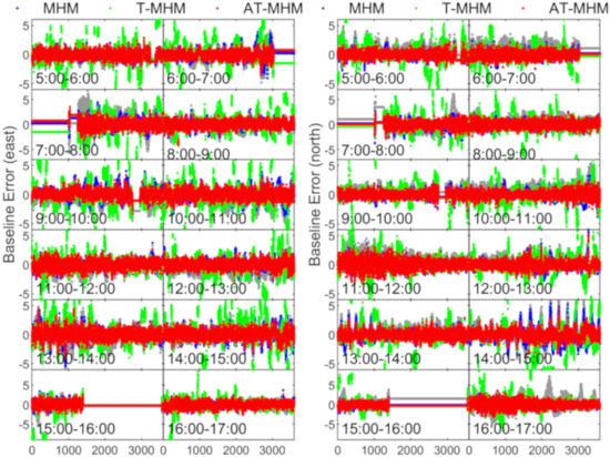
Figure 11.
The results of the east (left panel) and north (right panel) directions before and after the multipath correction on DOY51. The color gray in the figure indicates the uncorrected baseline solution of DOY 51. X-axis unit: second, Y-axis unit: meter.
Then, we continued to apply the DOY 50 model to DOY 52 multipath correction, and the results are shown in Table 7. From the perspective of the baseline accuracy improvement ratio, the correction ratio of MHM was slightly lower than that of DOY 50 and 51. The correction ratio of AT-MHM was basically stable except for a slight decrease in the north direction, while the overfitting of T-MHM was more serious. Figure 12 shows the comparison of the results of MHM and AT-MHM (east direction in the left panel and north direction in the right panel). As shown in the Figure 12, compared to MHM, the effect of AT-MHM on the high frequency multipath correction was still significant.
Table 7.
The RMSE of the uncorrected and the MHM, T-MHM, and AT-MHM corrected solutions on DOY52. (Unit: meter).
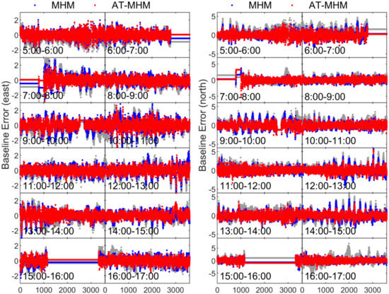
Figure 12.
The comparison between the MHM and AT-MHM multipath correction results of the east (left panel) and north (right panel) directions on DOY52. X-axis unit: second, Y-axis unit: meter.
4. Feasibility Discussion of Multipath Correction for Low-Cost Receiver
This experiment was to test the feasibility of applying the AT-MHM method to multipath reduction for a low-cost receiver in a strong multipath environment. We utilized the Ublox 9 receiver as the rover station to conduct a short baseline experiment at almost the same location as the previous year from DOY 152 to 153, 2020. The surrounding environment of the rover station is shown in Figure 13. The daily observation time was still from 5:00 to 17:00 UTC, covering a full 43,200 s with a sampling rate of 1 Hz. The base station also utilized the CORS station.
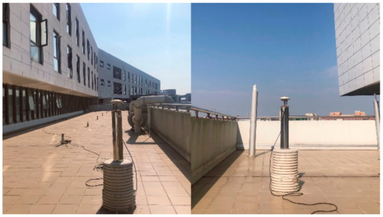
Figure 13.
The environment of the rover station of the Ublox test.
4.1. Multipath Error Assessment of Low-Cost Receiver
We evaluated the multipath error of the low-cost receiver in a similar environment as shown in Figure 14. The ZM single-difference of the Ublox test on DOY 153 were calculated, and the probability density diagram is shown in the left panel of Figure 14. We can see that the multipath value of this experiment was distributed between −76.5 and 314.3 m, of which 98.7% of the values fell between −10 and +10 m. We drew the skymap as shown in the right panel of Figure 14. The larger values were mostly distributed in the low-elevation area, which were interfered with by the reflected signal from the wall. Compared with those of the geodetic receiver, the pseudorange observations of the Ublox receiver suffered from greater multipath error and higher dispersion. Therefore, the application of AT-MHM to low-cost pseudorange multipath correction requires strong anti-noise ability.
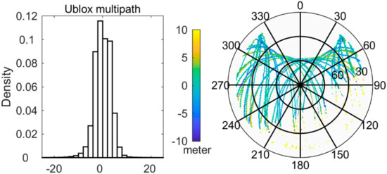
Figure 14.
The probability density histogram(left) and sky map(right) of the multipath error of DOY 153.
4.2. Comparison of MHM and AT-MHM in Double-Difference Mode for a Low-Cost Receiver
Since the effect of T-MHM on the pseudorange correction was discussed in terms of the geodetic receiver, we only discuss the correction results of the MHM and AT-MHM models in this section. We built correction models from DOY 152 and applied these to conduct multipath mitigation on DOY 153. The RMSE of the baseline solutions are shown in Table 8. The improvement ratios of AT-MHM and MHM were significantly higher than those of the geodetic receiver, because the power of pseudorange multipath of low-cost receiver was higher, and its low-frequency variation trend was well improved as shown in Figure 15. The fluctuation range and standard deviation of the baseline component corrected by AT-MHM were smaller. This is because the average value had only a small amount of correction for the grid points with a large multipath variation.
Table 8.
The multipath reduction effects of MHM and AT-MHM constructed from DOY 152 on DOY 153. (Unit: meter).
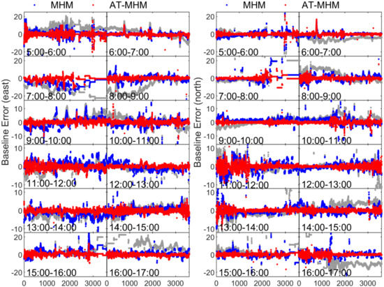
Figure 15.
Comparison of the multipath correction effect of MHM and AT-MHM modeled by DOY152 data on DOY153. Left panel, the east direction; Right panel, the north direction. X-axis unit: second, Y-axis unit: meter.
5. Conclusions
The multipath mitigation methods based on multipath spatial repeatability have the advantage of being able to be applied to static or dynamic environments in real-time correction. Among these. T-MHM utilizes the classical trend surface method to fit the multipath variation inside the grid. This has the advantages of enhancing the high-frequency multipath modeling capabilities. However, the application of trend surface analysis in T-MHM ignores the potential multicollinearity problem in the parameters and the influence of multipath anisotropy on the selection of the trend surface order, which makes the T-MHM method less capable of resisting the noise interference and limits its performance. This paper aimed to remedy the weakness in the application of T-MHM to express the spatial variation of the multipath error. An improved method named advanced trend surface analysis-based multipath hemispherical model (AT-MHM) was proposed to prevent multicollinearity of the parameters and to optimize the selection of the trend surface fitting forms.
The research work of this paper mainly contributes to the following four aspects: (1) We expounded the importance of preprocessing the multicollinearity problem of parameters in multipath trend surface fitting, and proposed a constraint scheme. (2) We proposed a new form of quadratic trend surface fitting considering the multipath anisotropy, which utilized the linear trend terms for parameters with weak spatial heterogeneity, thus, avoiding over interpretation of the spatial trend. Two typical cases were illustrated to verify the rationality and effectiveness of the improvement. (3) We extended AT-MHM to double-difference measure mode by utilizing the “Zero Mean” assumption to be adaptable for more general applications. (4) We verified the performance of pseudorange multipath correction for the geodetic receiver in a strong multipath environment and discussed the feasibility of multipath correction for low-cost equipment.
Short baseline experiments of both a geodetic receiver and low-cost receiver were conducted on a balcony near an office window, which can simulate the high shelter of a city environment and ensure a strong interference multipath error. This is a challenging but realistic application scene. In this environment, 98.5% of the ranging errors of the geodetic receiver fell in three meters, while 98.7% of the multipath values of the low-cost Ublox 9 receiver fell in 10 m. The performance of MHM, T-MHM, and AT-MHM were compared, and the results verify the fact that T-MHM suffered from overfitting due to relying on the goodness of fit and successive significance test to measure the accuracy of spatial trend predictions and that AT-MHM was more robust when the signal quality in a high-occlusion environment could not be guaranteed. AT-MHM could maximize the correction ability and avoid the overfitting result. Compared with the uncorrected solution, the accuracy of the MHM corrections were improved by approximately 33.6% for the Trimble receiver and 55.7% for the Ublox receiver. The enhancement ratios of the AT-MHM correction were approximately 45.7% for the Trimble receiver and 72.9% for the Ublox receiver.
Although, in this paper, we presented the multipath mitigation results of the MHM, T-MHM, and AT-MHM models for pseudorange observables in double-difference mode, this modeling method can also be extended in the following aspects. First, it can be applied to single station and dynamic scenes as long as the satellite clock, receiver clock, and other terms can be effectively solved. Second, AT-MHM can also be used for carrier multipath correction of low-cost devices theoretically. However, the premise of application is to ensure the carrier ambiguity is fixed accurately, which needs further study. Last, the modeling method based on multipath spatial repeatability only involves geometric repeatability of multipath signals. Therefore, it can also be applied to multi-constellation applications.
The reliability of the correction model, short sampling time, and applicability to real-time static or dynamic scenes are all advantages of AT-MHM, which is worthy of further study.
Author Contributions
Z.W., W.C., and D.D. conceived and designed the experiments; Z.W. performed the experiments; Z.W., W.C., C.Z., Y.P., and Z.Z. analyzed the data; Z.W., W.C., and D.D. wrote the paper; and all authors read the paper and provided revision suggestions. All authors have read and agreed to the published version of the manuscript.
Funding
This work was sponsored by the National Key R&D Program of China (No. 2017YFE0100700), the National Natural Science Foundation of China (No. 41771475, No. 61771197), and the Fund of Director of Key Laboratory of Geographic Information Science (Ministry of Education), East China Normal University (No. KLGIS2017C01).
Acknowledgments
The authors are grateful to the anonymous reviewers whose valuable comments greatly helped us to prepare an improved and clearer version of this paper. All persons and institutes who have kindly contributed to this analysis are acknowledged.
Conflicts of Interest
The authors declare no conflict of interest. The funders had no role in the design of the study; in the collection, analysis, or interpretation of data; in the writing of the manuscript, or in the decision to publish the results.
References
- Dinius, A.M. GPS antenna multipath rejection performance. Nasa Sti/Recon Tech. Rep. N. 1995, 96, 16–21. [Google Scholar]
- Nee, R.D.J.V. Multipath and Multi-Transmitter Interference in Spread-Spectrum Communication and Navigation Systems. Ph.D. Thesis, Delft University, Delft, The Netherlands, 23 May 1995. [Google Scholar]
- Van Nee, J.R.D.; Siereveld, J.; Fenton, P.C.; Townsend, B.R. The multipath estimating delay lock loop: Approaching theoretical accuracy limits. In Proceedings of the 1994 IEEE Position, Location and Navigation Symposium—PLANS’94, Las Vegas, NV, USA, 11–15 April 1994; pp. 246–251. [Google Scholar] [CrossRef]
- Van Dierendonck, A.J.; Fenton, P.; Ford, T. Theory and Performance of Narrow Correlator Spacing in a GPS Receiver. Navigation 1992, 39, 265–283. [Google Scholar] [CrossRef]
- Brown, A. Multipath rejection through spatial processing. In Proceedings of the 13th International Technical Meeting of the Satellite Division of The Institute of Navigation (ION GPS 2000), Salt Palace Convention Center, Salt Lake City, UT, USA, 19–22 September 2000; pp. 2330–2337. [Google Scholar]
- Ray, J.K.; Cannon, M.E.; Fenton, P. GPS code and carrier multipath mitigation using a multi-antenna system. IEEE Trans. Aerosp. Electron. Syst. 2001, 37, 183–195. [Google Scholar] [CrossRef]
- Fu, Z.; Hornbostel, A.; Hammesfahr, J.; Konovaltsev, A. Mitigation of multipath and jamming signals by digital beamforming for GPS/Galileo applications. Gps Solut. 2003, 6, 257–264. [Google Scholar] [CrossRef]
- Seco-Granados, G.; Fernandez-Rubio, J.; Fernandez-Prades, C. ML estimator and hybrid beamformer for multipath and interference mitigation in GNSS receivers. IEEE Trans. Signal Process. 2005, 53, 1194–1208. [Google Scholar] [CrossRef]
- Vicario, J.L.; Barcelo, M.; Seco-Granados, G.; Antreich, F.; Manuel Cebrian, J.; Picanyol, J.; Amarillo, F. A novel look into digital beamforming techniques for multipath and interference mitigation in Galileo Ground Stations. In Proceedings of the 2010 5th Advanced Satellite Multimedia Systems Conference and the 11th Signal Processing for Space Communications Workshop, Cagliari, Italy, 13–15 September 2010; pp. 240–247. [Google Scholar] [CrossRef]
- Manosas-Caballu, M.; Seco-Granados, G.; Swindlehurst, A.L. Robust beamforming via FIR filtering for GNSS multipath mitigation. In Proceedings of the 2013 IEEE International Conference on Acoustics, Speech and Signal Processing (ICASSP), Vancouver, BC, Canada, 26–31 May 2013; pp. 4173–4177. [Google Scholar]
- Manandhar, D.; Shibasaki, R.; Normark, P. GPS signal analysis using LHCP/RHCP antenna and software GPS receiver. In Proceedings of the 17th International Technical Meeting of the Satellite Division of The Institute of Navigation (ION GNSS 2004), Long Beach, CA, USA, 21−24 September 2004; pp. 2480–2498. [Google Scholar]
- Izadpanah, A. Parameterization of GPS L1 Multipath Using a dual Polarized RHCP/LHCP Antenna. Master’s Thesis, University of Calgary, Calgary, AB, Canada, 9 January 2009. [Google Scholar]
- Zhang, K.; Li, B.; Zhu, X.; Chen, H.; Sun, G. Multipath detection based on single orthogonal dual linear polarized GNSS antenna. Gps Solut. 2017, 21, 1203–1211. [Google Scholar] [CrossRef]
- Wieser, A.; Brunner, F.K. An extended weight model for GPS phase observations. Earthplanets Space 2000, 52, 777–782. [Google Scholar] [CrossRef]
- Groves, P.D.; Jiang, Z.; Rudi, M.; Strode, P. A Portfolio Approach to NLOS and Multipath Mitigation in Dense Urban Areas. In Proceedings of the 26th International Technical Meeting of the Satellite Division of The Institute of Navigation (ION GNSS+ 2013), Nashville, TN, USA, 16–20 September 2013; pp. 3231–3247. [Google Scholar]
- Zhong, P.; Ding, X.; Zheng, D.W.; Chen, W.; Huang, D.F. Adaptive wavelet transform based on cross-validation method and its application to GPS multipath mitigation. Gps Solut. 2007, 12, 109–117. [Google Scholar] [CrossRef]
- Satirapod, C.; Ogaja, C.; Wang, J.; Rizos, C. An approach to GPS analysis incorporating wavelet decomposition. J. Artif. Satell. 2001, 36, 27–35. [Google Scholar]
- Satirapod, C.; Rizos, C. Multipath mitigation by wavelet analysis for GPS base station applications. Surv. Rev. 2005, 38, 2–10. [Google Scholar] [CrossRef]
- Genrich, J.F.; Bock, Y. Rapid resolution of crustal motion at short ranges with the global positioning system. J. Geophys. Res. Space Phys. 1992, 97, 3261–3269. [Google Scholar] [CrossRef]
- Seeber, G.; Menge, F.; Völksen, C.; Wübbena, G.; Schmitz, M. Precise GPS Positioning Improvements by Reducing Antenna and Site Dependent Effects. In Advances in Positioning and Reference Frames; Springer: Berlin/Heidelberg, Germany, 1998; pp. 237–244. [Google Scholar]
- Choi, K.; Bilich, A.; Larson, K.M.; Axelrad, P. Modified sidereal filtering: Implications for high-rate GPS positioning. Geophys. Res. Lett. 2004, 31. [Google Scholar] [CrossRef]
- Ragheb, A.E.; Clarke, P.J.; Edwards, S.J. Coordinate-space and observation-space filtering methods for sidereally repeating errors in GPS: Performance and filter lifetime. In Proceedings of the 2007 National Technical Meeting of The Institute of Navigation, San Diego, CA, USA, 22–24 January 2007; pp. 480–485. [Google Scholar]
- Agnew, D.; Larson, K.M. Finding the repeat times of the GPS constellation. Gps Solut. 2006, 11, 71–76. [Google Scholar] [CrossRef]
- Zhong, P.; Ding, X.; Yuan, L.; Xu, Y.; Kwok, K.; Chen, Y. Sidereal filtering based on single differences for mitigating GPS multipath effects on short baselines. J. Geod. 2009, 84, 145–158. [Google Scholar] [CrossRef]
- Atkins, C.; Ziebart, M. Effectiveness of observation-domain sidereal filtering for GPS precise point positioning. Gps Solut. 2015, 20, 111–122. [Google Scholar] [CrossRef]
- Wang, M.; Wang, J.; Dong, D.; Li, H.; Han, L.; Chen, W. Comparison of Three Methods for Estimating GPS Multipath Repeat Time. Remote. Sens. 2018, 10, 6. [Google Scholar] [CrossRef]
- Wang, M.; Wang, J.; Dong, D.; Chen, W.; Li, H.; Wang, Z. Advanced Sidereal Filtering for Mitigating Multipath Effects in GNSS Short Baseline Positioning. Isprs. Int. J. Geo Inf. 2018, 7, 228. [Google Scholar] [CrossRef]
- Cohen, C.A.; Parkinson, B.W. Mitigating multipath error in GPS based attitude determination. Adv. Astronaut Sci. 1991, 74, 53–68. [Google Scholar]
- Dong, D.; Wang, M.; Chen, W.; Zeng, Z.; Song, L.; Zhang, Q.; Cai, M.; Cheng, Y.; Lv, J. Mitigation of multipath effect in GNSS short baseline positioning by the multipath hemispherical map. J. Geod. 2015, 90, 255–262. [Google Scholar] [CrossRef]
- Fuhrmann, T.; Luo, X.; Knöpfler, A.; Mayer, M. Generating statistically robust multipath stacking maps using congruent cells. Gps Solut. 2014, 19, 83–92. [Google Scholar] [CrossRef]
- Wang, Z.; Chen, W.; Dong, D.; Wang, M.; Cai, M.; Yu, C.; Zheng, Z.; Liu, M. Multipath mitigation based on trend surface analysis applied to dual-antenna receiver with common clock. Gps Solut. 2019, 23, 104. [Google Scholar] [CrossRef]
- Wheeler, D.; Tiefelsdorf, M. Multicollinearity and correlation among local regression coefficients in geographically weighted regression. J. Geogr. Syst. 2005, 7, 161–187. [Google Scholar] [CrossRef]
- Alber, C.; Ware, R.; Rocken, C.; Braun, J. Obtaining single path phase delays from GPS double differences. Geophys. Res. Lett. 2000, 27, 2661–2664. [Google Scholar] [CrossRef]
- Chayes, F. On deciding whether trend surfaces of progressively higher order are meaningful. Geol. Soc. Am. Bull. 1970, 81, 1273–1278. [Google Scholar] [CrossRef]
- Boots, B.; Tiefelsdorf, M. Global and local spatial autocorrelation in bounded regular tessellations. J. Geogr. Syst. 2000, 2, 319–348. [Google Scholar] [CrossRef]
- Pearson, W. Estimation of a correlation coefficient from an uncertainty measure. Psychometrika 1966, 31, 421–433. [Google Scholar] [CrossRef]


Publisher’s Note: MDPI stays neutral with regard to jurisdictional claims in published maps and institutional affiliations. |
© 2020 by the authors. Licensee MDPI, Basel, Switzerland. This article is an open access article distributed under the terms and conditions of the Creative Commons Attribution (CC BY) license (http://creativecommons.org/licenses/by/4.0/).