A Constrained Convex Optimization Approach to Hyperspectral Image Restoration with Hybrid Spatio-Spectral Regularization

Abstract

We propose a new constrained optimization approach to hyperspectral (HS) image restoration. Most existing methods restore a desirable HS image by solving some optimization problems, consisting of a regularization term(s) and a data-fidelity term(s). The methods have to handle a regularization term(s) and a data-fidelity term(s) simultaneously in one objective function; therefore, we need to carefully control the hyperparameter(s) that balances these terms. However, the setting of such hyperparameters is often a troublesome task because their suitable values depend strongly on the regularization terms adopted and the noise intensities on a given observation. Our proposed method is formulated as a convex optimization problem, utilizing a novel hybrid regularization technique named Hybrid Spatio-Spectral Total Variation (HSSTV) and incorporating data-fidelity as hard constraints. HSSTV has a strong noise and artifact removal ability while avoiding oversmoothing and spectral distortion, without combining other regularizations such as low-rank modeling-based ones. In addition, the constraint-type data-fidelity enables us to translate the hyperparameters that balance between regularization and data-fidelity to the upper bounds of the degree of data-fidelity that can be set in a much easier manner. We also develop an efficient algorithm based on the alternating direction method of multipliers (ADMM) to efficiently solve the optimization problem. We illustrate the advantages of the proposed method over various HS image restoration methods through comprehensive experiments, including state-of-the-art ones.

1. Introduction

Hyperspectral (HS) imagery has 1D spectral information, including invisible light and narrow wavelength interval, in addition to 2D spatial information and thus can visualize unseen intrinsic characteristics of scene objects and environmental lighting. This makes HS imaging a key technique in many applications in various fields, e.g., earth observation, agriculture, and medical and biological imaging [1,2,3].

Observed HS images are often affected by noise because of the small amount of light in narrow wavelength and/or sensor failure. In addition, in compressive HS imaging scenarios [4,5], we have to estimate a full HS image from a minimal number of measurements. Thus, we need some methods for restoring desirable HS images from such degraded observations in HS applications.

Most HS image restoration methods are established based on optimization: a desirable HS image is characterized as a solution to some optimization problem, which consists of a regularization term and a data-fidelity term. The regularization term evaluates apriori knowledge about underlying properties on HS images, and the data-fidelity term keeps the consistency with a given observation. Thanks to the design, these methods get a reasonable result under ill-posed or ill-conditioned scenarios typical in HS image restoration.

Regularization techniques for HS image restoration are roughly classified into two groups: total variation (TV)-based approach and low-rank modeling (LRM)-based one. TV models the total absolute magnitude of local differences to exploit the piecewise-smooth structures of an image. Many TV-based approaches [6,7,8,9] have been proposed for HS image restoration. Besides, LRM-based approaches [10,11] exploit the underlying low-rank structure in the spectral direction of an HS image. A popular example is the so-called Low-rank matrix recovery (LRMR) [10].

Many recent methods [9,12,13,14,15,16,17,18,19,20,21,22] combine TV-based and LRM-based approaches, and in general, they perform better than approaches using either regularization. This is because TV-based approaches model the spatial structure of an HS image, whereas LRM-based approaches the spectral one. Naturally, the methods have to handle multiple regularization terms and a data-fidelity term(s) simultaneously in one objective function. So the methods must carefully control the hyperparameter(s) balancing these terms. Specifically, such hyperparameters are interdependent, which means that a suitable value of a hyperparameter varies depending on the multiple regularization terms used and the noise intensities on a given observation. Hence, the hyperparameter settings in such combined approaches are often troublesome tasks.

Table 1. The feature of existing methods for hyperspectral (HS) image restoration.

	Feature	Spatial Correlation	Spectral Correlation	Convexity	Hyperparameters
Methods
HTV [6]		◯	×	convex	interdependent
SSAHTV [6]		◯	△	convex	interdependent
SSTV [7]		△	◯	convex	interdependent
ASSTV [8]		◯	◯	convex	interdependent
LRM [10,11]		×	◯	nonconvex	independent
LNWTV + LRM [9,12]		◯	◯	convex	interdependent
HTV + LRM [13]		◯	◯	nonconvex	interdependent
HTV + LRM [14,15]		◯	◯	convex	interdependent
ASSTV + LRM [16,17]		◯	◯	nonconvex	interdependent
SSTV + LRM [18,19,20]		◯	◯	convex	interdependent
SSTV + LRM [21,22]		◯	◯	nonconvex	interdependent
proposed		◯	◯	convex	independent

summarizes the features of the methods reviewed in this section.

Based on the above discussion, we propose a new constrained convex optimization approach to HS image restoration. Our proposed method restores a desirable HS image by solving a convex optimization problem involving a new TV-based regularization and hard constraints on data-fidelity. The regularization, named Hybrid Spatio-Spectral Total Variation (HSSTV), is designed to evaluate two types of local differences: direct local spatial differences and local spatio-spectral differences in a unified manner to effectively exploit both the underlying spatial and spectral structures of an HS image. Thanks to this design, HSSTV has a strong noise and artifact removal ability while avoiding oversmoothing and spectral distortion without combining LRM. Moreover, the constrained-type data-fidelity in the proposed method enables us to translate interdependent hyperparameters to the upper bounds of the degree of data-fidelity that can be determined based only on the noise intensity. As a result, the proposed method has no interdependent hyperparameter. We also develop an efficient algorithm for solving the optimization problem based on the well-known alternating direction method of multipliers (ADMM) [23,24,25].

The remainder of the paper is organized as follows. Section 2 introduces notation and mathematical ingredients. Section 3 reviews existing methods related to our method. In Section 4, we define HSSTV, formulate HS image restoration as a convex optimization problem involving HSSTV and hard-constraints on data-fidelity, and present an ADMM-based algorithm. Extensive experiments on denoising and compressed sensing (CS) reconstruction of HS images are given in Section 5, where we illustrate the advantages of our method over several state-of-the-art methods. In Section 6, we discuss the impact of the parameters in our proposed method. Section 7 concludes the paper. We have published the preliminary versions of this work in conference proceedings [26,27], including only limited experiments and discussions. In this paper, we newly conduct real noise removal experiments (see Section 5.2) and give much deeper discussions on the performance, utility, and parameter settings of the proposed method.

2. Preliminaries

2.1. Notation and Definitions

In this paper, let $\mathbb{R}$ be the set of real numbers. We shall use boldface lowercase and capital to represent vectors and matrices, respectively, and $:=$ to define something. We denote the transpose of a vector/matrix by ${(·)}^{\top }$, and the Euclidean norm (the ${\ell }_2$ norm) of a vector by $\parallel ·\parallel$.

For notational convenience, we treat an HS image $\mathcal{U}\in {\mathbb{R}}^{N_v\times N_h\times B}$ as a vector $\mathbf{u}\in {\mathbb{R}}^{NB}$ ($N:=N_v{N}_h$ is the number of the pixels of each band, and B is the number of the bands) by stacking its columns on top of one another, i.e., the index of the component of the ith pixel in kth band is $i+(k-1)N$ (for $i=1,\dots ,N$ and $k=1,\dots ,B$).

2.2. Proximal Tools

A function $f:{\mathbb{R}}^L\to (-\infty ,\infty ]$ is called proper lower semicontinuous convex if $dom\left(f\right):=\{\mathbf{x}\in {\mathbb{R}}^L|f\left(\mathbf{x}\right)<\infty \}\ne \varnothing$, ${lev}_{\le \alpha }\left(f\right):=\{\mathbf{x}\in {\mathbb{R}}^L|f\left(\mathbf{x}\right)\le \alpha \}$ is closed for every $\alpha \in \mathbb{R}$, and $f(\lambda \mathbf{x}+(1-\lambda \left)\mathbf{y}\right)\le \lambda f\left(\mathbf{x}\right)+(1-\lambda )f\left(\mathbf{y}\right)$ for every $\mathbf{x},\mathbf{y}\in {\mathbb{R}}^L$ and $\lambda \in (0,1)$, respectively. Let ${\mathsf{\Gamma }}_0\left({\mathbb{R}}^L\right)$ be the set of all proper lower semicontinuous convex functions on ${\mathbb{R}}^L$.

The proximity operator [28] plays a central role in convex optimization based on proximal splitting. The proximity operator of $f\in {\mathsf{\Gamma }}_0\left({\mathbb{R}}^L\right)$ with an index $\gamma >0$ is defined by

$${prox}_{\gamma f}\left(\mathbf{x}\right):=\underset{\mathbf{y}}{\mathrm{argmin}}f\left(\mathbf{y}\right)+\frac{1}{2\gamma }{\parallel \mathbf{y}-\mathbf{x}\parallel }^2.$$

We introduce the indicator function of a nonempty closed convex set $C\subset {\mathbb{R}}^L$, which is defined as follows:

$$\begin{array}{c}\hfill {\iota }_C\left(\mathbf{x}\right):=\left\{\begin{array}{cc}0,\hfill & \mathrm{if}\mathbf{x}\in C,\hfill \\ \infty ,\hfill & \mathrm{otherwise}.\hfill \end{array}\right.\end{array}$$

Then, for any $\gamma >0$, its proximity operator is given by

$${prox}_{\gamma {\iota }_C}\left(\mathbf{x}\right)=P_C\left(\mathbf{x}\right):=\underset{\mathbf{y}\in C}{\mathrm{argmin}}\parallel \mathbf{x}-\mathbf{y}\parallel ,$$

where $P_C\left(\mathbf{x}\right)$ is the metric projection onto C.

2.3. Alternating Direction Method of Multipliers (ADMM)

ADMM [23,24,25] is a popular proximal splitting method, and it can solve convex optimization problems of the form:

$$\underset{\mathbf{x},\mathbf{z}}{min}f\left(\mathbf{x}\right)+g\left(\mathbf{z}\right)\mathrm{s}.\mathrm{t}.\mathbf{z}=\mathbf{G}\mathbf{x},$$

(1)

where $f\in {\mathsf{\Gamma }}_0\left({\mathbb{R}}^{L_1}\right)$, $g\in {\mathsf{\Gamma }}_0\left({\mathbb{R}}^{L_2}\right)$, and $\mathbf{G}\in {\mathbb{R}}^{L_2\times L_1}$. Here, we assume that f is quadratic, g is proximable, i.e., the proximity operator of g is computable in an efficient manner, and $\mathbf{G}$ is a full-column rank matrix. For arbitrarily chosen ${\mathbf{z}}^{\left(0\right)},{\mathbf{d}}^{\left(0\right)}$ and a step size $\gamma >0$, ADMM iterates the following steps:

$$\begin{array}{c}\hfill ⌊\begin{array}{c}{\mathbf{x}}^{(n+1)}=\underset{\mathbf{x}}{\mathrm{argmin}}f\left(\mathbf{x}\right)+\frac{1}{2\gamma }{\parallel {\mathbf{z}}^{\left(n\right)}-\mathbf{G}\mathbf{x}-{\mathbf{d}}^{\left(n\right)}\parallel }^2,\hfill \\ {\mathbf{z}}^{(n+1)}={\mathrm{prox}}_{\gamma g}(\mathbf{G}{\mathbf{x}}^{(n+1)}+{\mathbf{d}}^{\left(n\right)}),\hfill \\ {\mathbf{d}}^{(n+1)}={\mathbf{d}}^{\left(n\right)}+\mathbf{G}{\mathbf{x}}^{(n+1)}-{\mathbf{z}}^{(n+1)},\hfill \end{array}\end{array}$$

(2)

The convergence property of ADMM is given as follows.

Theorem 1

(Convergence of ADMM [24]). Consider Problem (1), and assume that ${\mathbf{G}}^{\top }\mathbf{G}$ is invertible and that a saddle point of its unaugmented Lagrangian ${\mathcal{L}}_0(\mathbf{x},\mathbf{z},\mathbf{y}):=f\left(\mathbf{x}\right)+g\left(\mathbf{z}\right)-\langle \mathbf{d},\mathbf{G}\mathbf{x}-\mathbf{z}\rangle$ exists. A triplet $(\widehat{\mathbf{x}},\widehat{\mathbf{z}},\widehat{\mathbf{d}})$ is a saddle point of an unaugmented Lagrangian ${\mathcal{L}}_0$ if and only if ${\mathcal{L}}_0(\widehat{\mathbf{x}},\widehat{\mathbf{z}},\mathbf{d})\le {\mathcal{L}}_0(\widehat{\mathbf{x}},\widehat{\mathbf{z}},\widehat{\mathbf{d}})\le {\mathcal{L}}_0(\mathbf{x},\mathbf{z},\widehat{\mathbf{d}})$, for any $(\mathbf{x},\mathbf{z},\mathbf{d})\in {\mathbb{R}}^{L_1}\times {\mathbb{R}}^{L_2}\times {\mathbb{R}}^{L_2}$. Then the sequence ${\left({\mathbf{x}}_n\right)}_{n>0}$ generated by (2) converges to an optimal solution to Problem (1).

3. Related Works

In this section, we elaborate on existing HS image restoration methods based on optimization.

3.1. TV-Based Methods

The methods proposed in [6,7,8] restore a desirable HS image by solving a convex optimization problem involving TV-based regularization. Let $\overline{\mathbf{u}}\in {\mathbb{R}}^{NB}$ be the desirable HS image, and the authors assume that an observation $\mathbf{v}\in {\mathbb{R}}^{NB}$ is modeled as follows:

$$\mathbf{v}=\overline{\mathbf{u}}+\mathbf{s}+\mathbf{n},$$

where $\mathbf{n}$ and $\mathbf{s}$ are an additive white Gaussian noise and a sparse noise, respectively. Here, the sparse noise corrupts only a few pixels in the HS image but heavily, e.g., impulse noise, salt-and-pepper noise, and line noise. The observation and the restoration problem of the methods are given by the following forms:

$$\underset{\mathbf{u},\mathbf{s}}{min}{\parallel \mathbf{v}-\mathbf{u}-\mathbf{s}\parallel }^2+{\lambda }_1{\mathcal{R}}_{\mathrm{TV}}\left(\mathbf{u}\right)+{\lambda }_2{\parallel \mathbf{s}\parallel }_1,$$

(3)

where ${\mathcal{R}}_{\mathrm{TV}}$ is a regularization function based on TV, and ${\lambda }_1$ and ${\lambda }_2$ are hyperparameters. Here, The first and third terms evaluate data-fidelity on Gaussian and sparse noise, respectively. The hyperparameters ${\lambda }_1$ and ${\lambda }_2$ represent the priorities of each term. If we can choose suitable values of the hyperparameters, then this formulation yields high-quality restoration. However, the hyperparameters are interdependent, which means that suitable values of the hyperparameters vary depending on the used TV-based regularization term and the noise intensities on a given observation. Therefore, the settings of the hyperparameters are an essential but troublesome task.

In the following, we explain each TV. Let $\mathbf{D}={\left({\mathbf{D}}_v^{\top }{\mathbf{D}}_h^{\top }\right)}^{\top }\in {\mathbb{R}}^{2NB\times NB}$ be spatial differences operator with ${\mathbf{D}}_v$ and ${\mathbf{D}}_h$ being vertical and horizontal differences operator, respectively, and spectral differences operator are ${\mathbf{D}}_b\in {\mathbb{R}}^{NB\times NB}$. In [6,7,8], HTV, ASSTV, and SSTV are defined as follows:

$$\begin{array}{cc}\hfill HTV\left(\mathbf{u}\right)& :={\parallel \mathbf{D}\mathbf{u}\parallel }_{\mathrm{TV}},\hfill \end{array}$$

(4)

$$\begin{array}{cc}\hfill \mathrm{ASSTV}\left(\mathbf{u}\right)& :={\tau }_v\parallel {\mathbf{D}}_v{\mathbf{u}\parallel }_1+{\tau }_h\parallel {\mathbf{D}}_h{\mathbf{u}\parallel }_1+{\tau }_b{\parallel {\mathbf{D}}_b\mathbf{u}\parallel }_1,\hfill \end{array}$$

(5)

$$\begin{array}{cc}\hfill SSTV\left(\mathbf{u}\right)& :=\parallel \mathbf{D}{\mathbf{D}}_b{\mathbf{u}\parallel }_1,\hfill \end{array}$$

(6)

where ${\parallel ·\parallel }_{\mathrm{TV}}$ is a TV norm, which takes the ${\ell }_2$ norm of spacial difference vectors for all band and then summing up for all spatial pixels, and ${\tau }_v$, ${\tau }_h$, and ${\tau }_b$ are the weight of the vertical, horizontal, and spectral differences. HTV evaluates direct spatial piecewise-smoothness and can be seen as a generalization of the standard color TV [29]. HTV does not consider spectral correlation, resulting in spatial oversmoothing. To consider the spectral correlation, the authors of [6] proposed SSAHTV. SSAHTV is a weighted HTV, and the weight is determined by spectral information. However, since SSAHTV does not directly evaluate spectral correlation, it still causes spatial oversmoothing. ASSTV evaluates direct spatial and spectral piecewise-smoothness (Figure 1, blue line). The weights ${\tau }_v$, ${\tau }_h$, and ${\tau }_b$ in (5) balance the smoothness of vertical, horizontal, and spectral differences, respectively. Owing to the definition, ASSTV can evaluate spatial and spectral correlation, but it produces spectral oversmoothing even if we carefully adjust ${\tau }_v$, ${\tau }_h$, and ${\tau }_b$. SSTV evaluate a-prior knowledge on HS images using spatio-spectral piecewise-smoothness. It is derived by calculating spatial differences through spectral differences (Figure 1, yellow line). SSTV can restore a desirable HS image without any weight, but it produces noise-like artifacts, especially when a given observation is contaminated by heavy noise and/or degradation.

3.2. LRM-Based Method

LRMR [10] is one of the popular LRM-based methods for HS image restoration, which evaluates the low rankness of an HS image in the spectral direction. To preserve the local details, LRMR restores a desirable HS image through patch-wise processing. Each patch is a local cube of the size of $q\times q\times B$, and LRMR handles it as a matrix of size $q^2\times B$ obtained by lexicographically arranging the spatial vectors in the patch cube in the row direction. The observation model is expressed like Section 3.1, and the restoration problem is formulated as follows:

$$\underset{{\mathbf{U}}_{i,j},{\mathbf{S}}_{i,j}}{min}{\parallel {\mathbf{V}}_{i,j}-{\mathbf{U}}_{i,j}-{\mathbf{S}}_{i,j}\parallel }_F^2\mathrm{s}.\mathrm{t}.rank\left({\mathbf{U}}_{i,j}\right)\le r,card\left({\mathbf{S}}_{i,j}\right)\le k,$$

(7)

where ${\mathbf{U}}_{i,j}$, ${\mathbf{V}}_{i,j}$, and ${\mathbf{S}}_{i,j}$ represent the patches of a restored HS image, an observation, and a sparse noise, respectively, which are centered at (i,j) pixel. Then, the ${\parallel ·\parallel }_F$ is a Frobenius norm, $rank(·)$ represents a rank function, and $card(·)$ is a cardinality function. The method evaluates the low rankness of the estimated HS image and sparsity of the sparse noise by limiting the number of the rank of ${\mathbf{U}}_{i,j}$ and the cardinality of ${\mathbf{S}}_{i,j}$ using r and k, respectively. Thanks to the design, LRMR achieves high-quality restoration for especially spectral information. Meanwhile, since LRMR does not fully consider spatial correlation, the result by LRMR tends to have spatial artifacts when an observation is corrupted by heavy noise and/or degradation. Besides, the rank and cardinality functions are nonconvex, and so it is a troublesome task to seek the global optimal solution of Problem (7).

3.3. Combined Method

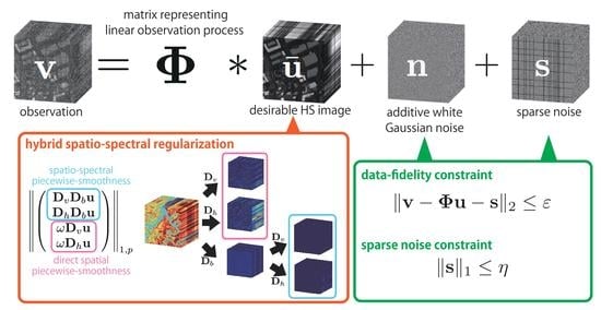
The methods [9,12,13,14,15,16,17,18,19,20,21,22,30] combine TV-based and LRM-based approaches. Since they can evaluate multiple types of apriori knowledge, i.e., piecewise-smoothness and low rankness, they can restore a more desirable HS image than the approaches only using TV-based or LRM-based regularization. Some methods [9,12,14,15,17,18,19,20] approximate the rank and cardinality functions by their convex surrogates. As a result, the restoration problems are convex and can be solved by optimization methods based on proximal splitting.

However, the methods have to handle multiple regularization terms and/or a data-fidelity term(s) simultaneously in one objective function; they require to carefully control the hyperparameters balancing these terms. Since the hyperparameters rely on both the regularizations and the noise intensity on an observation, i.e., the hyperparameters are interdependent, the hyperparameter settings are often troublesome tasks.

4. Proposed

4.1. Hybrid Spatio-Spectral Total Variation

We propose a new regularization technique for HS image restoration, named HSSTV. HSSTV simultaneously handles both direct local spatial differences and local spatio-spectral differences of an HS image. Then, HSSTV is defined by

$$HSSTV\left(\mathbf{u}\right):=\parallel {\mathbf{A}}_{\omega }{\mathbf{u}\parallel }_{1,p}\mathrm{with}{\mathbf{A}}_{\omega }:=\left(\begin{array}{c}\mathbf{D}{\mathbf{D}}_b\\ \omega \mathbf{D}\end{array}\right),$$

(8)

where ${\parallel ·\parallel }_{1,p}$ is the mixed ${\ell }_{1,p}$ norm, and $\omega \ge 0$. We assume $p=1$ or 2, i.e., the ${\ell }_1$ norm (${\parallel ·\parallel }_{1,1}={\parallel ·\parallel }_1$) or the mixed ${\ell }_{1,2}$ norm, respectively. We would like to mention that we can also see ${\ell }_1$-HSSTV ($p=1$) as anisotropic HSSTV and ${\ell }_{1,2}$-HSSTV ($p=2$) as isotropic HSSTV.

In (8), $\mathbf{D}{\mathbf{D}}_b\mathbf{u}$ and $\mathbf{D}\mathbf{u}$ correspond to local spatio-spectral and direct local spatial differences, respectively, as shown in Figure 1 (red lines). The weight $\omega$ adjusts the relative importance of direct spatial piecewise-smoothness to spatio-spectral piecewise-smoothness. HSSTV evaluates two kinds of smoothness by taking the ${\ell }_p$ norm ($p=1$ or 2) of these differences associated with each pixel and then summing up for all pixels, i.e., calculating the ${\ell }_1$ norm. Thus, it can be defined via the mixed ${\ell }_{1,p}$ norm. When we set $\omega =0$ and $p=1$, HSSTV recovers SSTV as (6), meaning that HSSTV can be seen as a generalization of SSTV.

As reviewed in Section 3, since SSTV only evaluates spatio-spectral piecewise-smoothness, it cannot remove similar noise in adjacent bands. The direct spatial differences in HSSTV help to remove such noise. Figure 2 is restored HS images from an observation contaminated by similar noise in adjacent bands (the upper half area) and random noise (the lower half area). One can see that large noise remains in the upper half area of the result by SSTV. In contrast, HSSTV effectively removes all noise. However, since minimizing the direct spatial differences strongly promotes spatial piecewise-smoothness, HSSTV produces spatial oversmoothing when the weight $\omega$ is large. Thus, the weight $\omega$ should be set to less than one, as demonstrated in Section 5.

4.2. HS Image Restoration by HSSTV

We consider restoring a desirable HS image $\overline{\mathbf{u}}\in {\mathbb{R}}^{NB}$ from an observation $\mathbf{v}\in {\mathbb{R}}^M(M\le NB)$ contaminated by a Gaussian-sparse mixed noise. The observation model is given by the following form:

$$\mathbf{v}=\mathsf{\Phi }\overline{\mathbf{u}}+\mathbf{n}+\mathbf{s},$$

(9)

where $\mathsf{\Phi }\in {\mathbb{R}}^{M\times NB}$ is a matrix representing a linear observation process, e.g., random sampling, $\mathbf{n}\in {\mathbb{R}}^M$ is Gaussian noise with the standard deviation $\sigma$, and $\mathbf{s}\in {\mathbb{R}}^M$ is a sparse noise.

Based on the above model, we formulate HS image restoration using HSSTV as the following optimization problem:

$$\begin{array}{cc}\hfill & \underset{\mathbf{u},\mathbf{s}}{min}HSSTV\left(\mathbf{u}\right)\mathrm{s}.\mathrm{t}.\left[\begin{array}{c}\mathsf{\Phi }\mathbf{u}+\mathbf{s}\in {\mathcal{B}}_{2,\epsilon }^{\mathbf{v}}:=\{\mathbf{x}\in {\mathbb{R}}^M|\parallel \mathbf{v}-\mathbf{x}\parallel \le \epsilon \},\hfill \\ \mathbf{s}\in {\mathcal{B}}_{1,\eta }:=\{\mathbf{x}\in {\mathbb{R}}^M{|\parallel \mathbf{x}\parallel }_1\le \eta \},\hfill \\ \mathbf{u}\in {[{\mu }_{min},{\mu }_{max}]}^{NB},\hfill \end{array}\right.\hfill \end{array}$$

(10)

where ${\mathcal{B}}_{2,\epsilon }^{\mathbf{v}}$ is a $\mathbf{v}$-centered ${\ell }_2$-norm ball with the radius $\epsilon >0$, ${\mathcal{B}}_{1,\eta }$ is a $\mathbf{0}$-centered ${\ell }_1$-norm ball with the radius $\eta >0$, and ${[{\mu }_{min},{\mu }_{max}]}^{NB}$ is a dynamic range of an HS image (${\mu }_{min}<{\mu }_{max}$). This method simultaneously estimates the desirable HS image $\mathbf{u}$ and the sparse noise $\mathbf{s}$ for noise-robust restoration. The first and second constraints measure data fidelities to the observation $\mathbf{v}$ and the sparse noise $\mathbf{s}$, respectively. As mentioned in [13,16,26,31,32,33,34,35,36,37,38,39], such a constraint-type data-fidelity enables us to translate the hyperparameter(s) balancing between regularization and data-fidelity like ${\lambda }_1$ and ${\lambda }_2$ in (3) to the upper bound of the degree of data-fidelity $\epsilon$ and $\eta$ that can be set in a much easier manner.

Since all constraints are closed convex sets and HSSTV is a convex function, Problem (10) is a constrained convex optimization problem. In this paper, we adopt ADMM (see Section 2.3) for solving the problem. In what follows, we reformulate Problem (10) into Problem (1).

By using the indicator functions of the constraints, Problem (10) can be rewritten as

$$\underset{\mathbf{u},\mathbf{s}}{min}{\parallel {\mathbf{A}}_{\omega }\mathbf{u}\parallel }_{1,p}+{\iota }_{{\mathcal{B}}_{2,\epsilon }^{\mathbf{v}}}(\mathsf{\Phi }\mathbf{u}+\mathbf{s})+{\iota }_{{\mathcal{B}}_{1,\eta }}\left(\mathbf{s}\right)+{\iota }_{{[{\mu }_{min},{\mu }_{max}]}^{NB}}\left(\mathbf{u}\right).$$

(11)

Note that from the definition of the indicator function, Problem (11) is exactly equal to Problem (10). By letting

$$\begin{array}{ll}\hfill f:& {\mathbb{R}}^{NB}\to {\mathbb{R}}^2:\mathbf{u}\mapsto (0,0),\hfill \end{array}$$

(12)

$$\begin{array}{ll}\hfill g:& {\mathbb{R}}^{5NB+2M}\to \mathbb{R}\cup \{\infty \}:({\mathbf{z}}_1,{\mathbf{z}}_2,{\mathbf{z}}_3,{\mathbf{z}}_4)\mapsto {\parallel {\mathbf{z}}_1\parallel }_{1,p}+{\iota }_{{\mathcal{B}}_{2,\epsilon }^{\mathbf{v}}}\left({\mathbf{z}}_2\right)+{\iota }_{{\mathcal{B}}_{1,\epsilon }}\left({\mathbf{z}}_3\right)+{\iota }_{{[{\mu }_{min},{\mu }_{max}]}^{NB}}\left({\mathbf{z}}_4\right),\hfill \end{array}$$

(13)

$$\begin{array}{ll}\hfill \mathbf{G}:& {\mathbb{R}}^{NB}\to {\mathbb{R}}^{5NB+2M}:\mathbf{u}\mapsto ({\mathbf{A}}_{\omega }\mathbf{u},\mathsf{\Phi }\mathbf{u}+\mathbf{s},\mathbf{s},\mathbf{u}).\hfill \end{array}$$

(14)

Problem (11) is reduced to Problem (1). The resulting algorithm based on ADMM is summarized in Algorithm 1.

Algorithm 1: ADMM method for Problem (10)

The update of $\mathbf{u}$ and $\mathbf{s}$ in Algorithm 1 comes down to the following forms:

$$\begin{array}{cc}\hfill {\mathbf{u}}^{(n+1)}=& {\left({\mathbf{A}}_{\omega }^{\top }{\mathbf{A}}_{\omega }+{\mathsf{\Phi }}^{\top }\mathsf{\Phi }+\frac{1}{2}\mathbf{I}\right)}^{-1}RHS,\hfill \\ \hfill RHS=& {\mathbf{A}}_{\omega }^{\top }({\mathbf{z}}_1^{\left(n\right)}-{\mathbf{d}}_1^{\left(n\right)})+\frac{1}{2}{\mathsf{\Phi }}^{\top }({\mathbf{z}}_2^{\left(n\right)}-{\mathbf{d}}_2^{\left(n\right)})-\frac{1}{2}({\mathbf{z}}_3^{\left(n\right)}-{\mathbf{d}}_3^{\left(n\right)})+({\mathbf{z}}_4^{\left(n\right)}-{\mathbf{d}}_4^{\left(n\right)}),\hfill \\ \hfill {\mathbf{s}}^{(n+1)}=& \frac{1}{2}({\mathbf{z}}_2^{\left(n\right)}-{\mathbf{u}}^{(n+1)}-{\mathbf{d}}_2^{\left(n\right)}+{\mathbf{z}}_3^{\left(n\right)}-{\mathbf{d}}_3^{\left(n\right)}),\hfill \end{array}$$

(15)

Since the update of $\mathbf{u}$ and $\mathbf{s}$ in Algorithm 1 is strictly-convex quadratic minimization, one can obtain these updated forms by differentiating it. Here, we should consider the structure of $\mathsf{\Phi }$ because it affects the matrix inversion in (15). If $\mathsf{\Phi }$ is a block-circulant-with-circulant-blocks (BCCB) matrix [40], we can leverage 3DFFT to efficiently solve the inversion in Step 2 with the difference operators having a periodic boundary, i.e., ${\mathbf{A}}_{\omega }^{\top }{\mathbf{A}}_{\omega }+{\mathsf{\Phi }}^{\top }\mathsf{\Phi }+\mathbf{I}$ can be diagonalized by the 3D FFT matrix and its inverse. If $\mathsf{\Phi }$ is a semiorthogonal matrix, i.e., $\mathsf{\Phi }{\mathsf{\Phi }}^{\top }=\alpha \mathbf{I}$$(\alpha >0)$, we leave it to the update of ${\mathbf{z}}_2$, which means that we replace ${\iota }_{{\mathcal{B}}_{2,\epsilon }^{\mathbf{v}}}$ by ${\iota }_{{\mathcal{B}}_{2,\epsilon }^{\mathbf{v}}}\circ \mathsf{\Phi }$ in (13) and $\mathsf{\Phi }\mathbf{u}$ by $\mathbf{u}$ in (14). This is because the proximity operator of ${\iota }_{{\mathcal{B}}_{2,\epsilon }^{\mathbf{v}}}\circ \mathsf{\Phi }$, in this case, can be computed by using [41] (Table 1.1-x) as follows:

$${prox}_{\gamma {\iota }_{{\mathcal{B}}_{2,\epsilon }^{\mathbf{v}}}\circ \mathsf{\Phi }}\left(\mathbf{x}\right)=\mathbf{x}+{\alpha }^{-1}{\mathsf{\Phi }}^{\top }(P_{{\mathcal{B}}_{2,\epsilon }^{\mathbf{v}}}\left(\mathsf{\Phi }\mathbf{x}\right)-\mathsf{\Phi }\mathbf{x}).$$

If $\mathsf{\Phi }$ is a sparse matrix, we offer to use a preconditioned conjugate gradient method [42] for approximately solving the inversion or to apply primal-dual splitting methods [43,44,45] instead of ADMM (Primal-dual splitting methods require no matrix inversion but in general their convergence speed is slower than ADMM. Otherwise, randomized image restoration methods using stochastic proximal splitting algorithms [46,47,48,49] might be useful for reducing the computational cost.

For the update of ${\mathbf{z}}_1$, the proximity operators are reduced to simple soft-thresholding type operations: for $\gamma >0$ and for $i=1,\dots ,4NB$, (i) in the case of $p=1$,

$${\left[{prox}_{{\gamma \parallel ·\parallel }_1}\left(\mathbf{x}\right)\right]}_i=sgn\left(x_i\right)max\left\{|x_i|-\gamma ,0\right\},$$

where sgn is the sign function, and (ii) in the case of $p=2$,

$${\left[{prox}_{{\gamma \parallel ·\parallel }_{1,2}}\left(\mathbf{x}\right)\right]}_i=max\left\{1-\gamma {\left(\sum _{j=0}^3{x}_{\tilde{i}+jNB}^2\right)}^{-\frac{1}{2}},0\right\}{x}_i,$$

where $\tilde{i}:=((i-1)modNB)+1$.

The updates of ${\mathbf{z}}_2$, ${\mathbf{z}}_3$, and ${\mathbf{z}}_4$ require the proximity operators of the indicator functions of ${\mathcal{B}}_{2,\epsilon }^{\mathbf{v}}$, ${\mathcal{B}}_{1,\eta }$, and ${[{\mu }_{min},{\mu }_{max}]}^{NB}$, respectively, which equate the metric projections onto them (see Section 2.2). Specifically, the metric projection to ${\mathcal{B}}_{2,\epsilon }^{\mathbf{v}}$ is given by

$$P_{{\mathcal{B}}_{2,\epsilon }^{\mathbf{v}}}\left(\mathbf{x}\right)=\left\{\begin{array}{cc}\mathbf{x},\hfill & \mathrm{if}\mathbf{x}\in {\mathcal{B}}_{2,\epsilon }^{\mathbf{v}},\hfill \\ \mathbf{v}+\frac{\epsilon (\mathbf{x}-\mathbf{v})}{\parallel \mathbf{x}-\mathbf{v}\parallel },\hfill & \mathrm{otherwise},\hfill \end{array}\right.$$

that onto ${\mathcal{B}}_{1,\eta }$ is given by

$$P_{{\mathcal{B}}_{1,\eta }}=sgn\left(\mathbf{x}\right)max\left(\right|\mathbf{x}|-\eta ,0),$$

and that onto ${[{\mu }_{min},{\mu }_{max}]}^{NB}$ is given, for $i=1,\dots ,NB$, by

$${\left[P_{{[{\mu }_{min},{\mu }_{max}]}^{NB}}\left(\mathbf{x}\right)\right]}_i=min\{max\{x_i,{\mu }_{min}\},{\mu }_{max}\}.$$

5. Results

We demonstrate the advantages of the proposed method by applying it to two specific HS image restoration problems: denoising and CS reconstruction. In these experiments, we used 13 HS images taken from the SpecTIR [50], MultiSpec [51], and GIC [52], with their dynamic ranges normalized into $[0,1]$. All the experiments were conducted by MATLAB 2018a.

The proposed method was compared with HTV [6], SSAHTV [6], SSTV [7], and ASSTV [38]. For a fair comparison, we replaced HSSTV in Problem (10) with HTV, SSAHTV, SSTV, or ASSTV and solved the problem by ADMM. In the denoising experiments, we also compared our proposed method with LRMR [10], TV-regularized low-rank matrix factorization (LRTV) [13], and local low-rank matrix recovery and global spatial-spectral TV (LLRGTV) [16]. Since LRMR, LRTV, and LLRGTV are customized to the mixed noise removal problem, we cannot adopt them for CS reconstruction. We did not compare our proposed method with recent CNN-based HS image denoising methods [53,54]. The CNN-based methods cannot be represented as explicit regularization functions and are fully customized to denoising tasks. In contrast, our proposed method can be used as a building block in various HS image restoration methods based on optimization. Meanwhile, CNN-based methods strongly depend on what training data are used, which means that they cannot adapt to a wide range of noise intensity. Thus, the design concepts of these methods are different from TVs and LRM-based approaches.

To quantitatively evaluate restoration performance, we used the peak signal-to-noise ratio (PSNR) [dB] index and the structural similarity (SSIM) [55] index between a groundtruth HS image $\overline{\mathbf{u}}$ and a restored HS image $\mathbf{u}$. PSNR is defined by $10{log}_{10}(MA{X}_I^2/MSE)$, where $MA{X}_I$ is the max value of the dynamic range of HS images, and $MSE$ is the mean square error between groundtruth HS images and restored HS images. The higher PSNR is, the more similar the two images are. SSIM is an image quality assessment index based on the human vision system, which is defined as follows:

$$\begin{array}{cc}\hfill \mathrm{SSIM}(\mathbf{u},\overline{\mathbf{u}})& =\frac{1}{P}\sum _{i=1}^P{\mathrm{SSIM}}_i(\mathbf{u},\overline{\mathbf{u}}),\hfill \\ \hfill {\mathrm{SSIM}}_i(\mathbf{u},\overline{\mathbf{u}})& =\frac{(2{\mu }_{{\mathbf{u}}_i}{\mu }_{{\overline{\mathbf{u}}}_i}+C_1)(2{\sigma }_{{\mathbf{u}}_i{\overline{\mathbf{u}}}_i}+C_2)}{({\mu }_{{\mathbf{u}}_i}^2+{\mu }_{{\overline{\mathbf{u}}}_i}^2+C_1)({\sigma }_{{\mathbf{u}}_i}^2+{\sigma }_{{\overline{\mathbf{u}}}_i}^2+C_2)},\hfill \end{array}$$

where ${\mathbf{u}}_i$ and ${\overline{\mathbf{u}}}_i$ are the ith pixel-centered local patches of a restored HS image and a groundtruth HS image, respectively, P is the number of patches, ${\mu }_{{\mathbf{u}}_i}$ and ${\mu }_{{\overline{\mathbf{u}}}_i}$ is the average values of the local patches of the restored and groundtruth HS images, respectively, ${\sigma }_{{\mathbf{u}}_i}$ and ${\sigma }_{{\overline{\mathbf{u}}}_i}$ represent the variances of ${\mathbf{u}}_i$ and ${\overline{\mathbf{u}}}_i$, respectively, and ${\sigma }_{{\mathbf{u}}_i{\overline{\mathbf{u}}}_i}$ denotes the covariance between ${\mathbf{u}}_i$ and ${\overline{\mathbf{u}}}_i$. Moreover, $C_1$ and $C_2$ are two constants, which avoid the numerical instability when either ${\mu }_{{\mathbf{u}}_i}^2+{\mu }_{{\overline{\mathbf{u}}}_i}^2$ or ${\sigma }_{{\mathbf{u}}_i}^2+{\sigma }_{{\overline{\mathbf{u}}}_i}^2$ is very close to zero. SSIM gives a normalized score between zero and one, where the maximum value means that $\mathbf{u}$ equals to $\overline{\mathbf{u}}$.

We set the max iteration number, the stepsize $\gamma$, and the stopping criterion of ADMM to 10,000, 0.05, and $\parallel {\mathbf{u}}^{\left(n\right)}-{\mathbf{u}}^{(n+1)}\parallel <0.01$, respectively.

5.1. Denoising

First, we experimented on the Gaussian-sparse mixed noise removal of HS images. The observed HS images included an additive white Gaussian noise $\mathbf{n}$ with the standard deviation $\sigma$ and sparse noise $\mathbf{s}$. In these experiments, we assumed that sparse noise consists of salt-and-pepper noise and vertical and horizontal line noise, with these noise ratio in all pixels being $s_p$, $l_v$, and $l_h$, respectively. We generated noisy HS images by adding two types of mixed noise to groundtruth HS images: (i) $(\sigma ,s_p,l_v=l_h)=(0.05,0.04,0.04)$, (ii) $(0.1,0.05,0.05)$. In the denoising case, $\mathsf{\Phi }=\mathbf{I}$ in (9), and the radiuses $\epsilon$ and $\eta$ in Problem (10) were set to $0.83\sqrt{NB(1-(s_p(1-l_v-l_h)+l_v+l_h-l_v{l}_h)){\sigma }^2}$ and $NB(0.45s_p+(l_v+l_h)v_{ave}-l_v{l}_h{v}_{ave})$, respectively, where $v_{ave}$ is the average of the observed image.

Table 2. Parameter settings for ASSTV, LRMR, LRTV, and the proposed method.

	Noise Level	(i) $(\mathit{\sigma },{\mathit{s}}_{\mathit{p}},{\mathit{l}}_{\mathit{v}}={\mathit{l}}_{\mathit{h}})=(0.05,0.04,0.04)$	(ii) $(0.1,0.05,0.05)$
Parameters
ASSTV	${\tau }_v={\tau }_h$	1	1
	${\tau }_b$	3	2
LRMR	r	3	3
	k	$s_p+l_v+l_h-l_v{l}_h$ (the rate of sparse noise)
LRTV	r	2	2
	$\tau$	0.005	0.008
LLRGTV	r	2	2
	$\lambda$	0.1	0.1
	$\tau$	0.01	0.01
proposed	$\omega$	0.04	0.04

shows the parameters settings for ASSTV, LRMR, LRTV, LLRGTV, and the proposed method. We set these parameters to achieve the best performance for each method.

In

Table 3. Peak signal-to-noise ratio (PSNR) (top) and structural similarity (SSIM) (bottom) in mixed noise removal experiments.

	HS Image	Noise Level	HTV	SSAHTV	SSTV	ASSTV	LRMR	LRTV	LLRGTV	Proposed ($\mathit{p}=1$)	Proposed ($\mathit{p}=2$)
	Beltsville	(i)	29.43	29.47	33.66	27.16	30.91	35.32	33.61	34.25	34.16
	$256\times 256\times 32$	(ii)	26.40	26.43	28.42	24.60	27.13	31.22	28.51	29.79	29.62
	Suwannee	(i)	30.14	30.18	34.59	32.60	30.30	36.20	33.35	35.15	36.01
	$256\times 256\times 32$	(ii)	26.70	26.74	29.55	28.71	26.90	31.95	28.50	31.08	31.22
	DC	(i)	26.46	26.51	33.03	28.80	31.71	34.78	33.50	33.36	33.08
	$256\times 256\times 32$	(ii)	23.84	23.88	27.71	25.25	27.35	29.53	28.14	28.57	28.32
	Cuprite	(i)	31.67	31.68	34.42	29.14	30.16	28.39	32.67	34.96	36.20
	$256\times 256\times 32$	(ii)	28.20	28.21	29.86	26.57	27.32	27.94	27.99	31.63	31.73
	Reno	(i)	28.53	28.57	34.37	30.49	32.21	37.06	34.95	35.11	34.96
	$256\times 256\times 32$	(ii)	25.56	25.61	28.11	26.95	28.47	31.00	27.99	29.83	29.72
	Botswana	(i)	27.98	28.05	33.32	26.47	31.62	29.00	32.02	33.61	33.53
	$256\times 256\times 32$	(ii)	25.21	25.25	28.55	24.01	28.31	27.33	28.08	29.39	29.35
PSNR	IndianPines	(i)	31.05	31.06	31.45	29.07	28.96	26.16	29.74	31.90	31.80
	$145\times 145\times 32$	(ii)	28.57	28.57	27.82	26.72	25.14	29.82	26.70	29.26	29.18
	KSC	(i)	30.17	30.25	34.74	31.64	33.74	35.74	34.75	36.39	36.33
	$256\times 256\times 32$	(ii)	28.03	28.06	29.23	28.62	30.19	30.22	29.53	31.82	31.72
	PaviaLeft	(i)	27.62	27.70	35.57	30.91	33.01	36.49	34.75	35.98	35.81
	$216\times 216\times 32$	(ii)	24.74	24.78	29.93	26.71	29.46	29.02	29.22	30.47	30.24
	PaviaRight	(i)	26.93	27.35	34.54	31.13	33.33	35.82	34.17	35.68	35.23
	$256\times 256\times 32$	(ii)	24.90	25.16	30.70	27.23	29.82	29.08	29.24	31.59	31.39
	PaviaU	(i)	27.92	28.04	35.52	31.65	33.00	36.72	34.59	36.31	36.17
	$256\times 256\times 32$	(ii)	25.24	25.29	30.21	27.42	29.43	28.90	29.17	31.04	30.80
	Salinas	(i)	32.59	32.64	35.86	32.83	31.82	36.74	34.36	37.60	37.65
	$217\times 217\times 32$	(ii)	28.88	28.91	28.19	28.99	28.02	32.73	29.09	32.01	32.12
	SalinaA	(i)	32.54	32.65	35.29	28.12	31.18	28.49	34.07	36.27	36.23
	$83\times 86\times 32$	(ii)	28.69	28.80	29.67	25.19	27.67	26.10	27.87	31.68	31.64
	Beltsville	(i)	0.7902	0.7904	0.8856	0.8111	0.8583	0.9372	0.9278	0.9132	0.9085
		(ii)	0.6954	0.6959	0.7057	0.7177	0.7083	0.8568	0.8248	0.8186	0.8088
	Suwannee	(i)	0.8406	0.8410	0.9353	0.9052	0.8689	0.9502	0.9431	0.9559	0.9555
		(ii)	0.7542	0.7552	0.8146	0.8226	0.7470	0.8930	0.8622	0.9125	0.9158
	DC	(i)	0.7622	0.7633	0.9274	0.8676	0.9248	0.9613	0.9548	0.9442	0.9394
		(ii)	0.6189	0.6201	0.8092	0.7211	0.8214	0.8810	0.8722	0.8611	0.8533
	Cuprite	(i)	0.8550	0.8552	0.9179	0.8632	0.8495	0.9396	0.9411	0.9459	0.9426
		(ii)	0.7849	0.7852	0.7717	0.7953	0.7098	0.8814	0.8524	0.9031	0.9058
	Reno	(i)	0.7818	0.7819	0.9322	0.8832	0.9012	0.9589	0.9523	0.9531	0.9515
		(ii)	0.6640	0.6645	0.8045	0.7539	0.7905	0.8816	0.8640	0.8679	0.8635
	Botswana	(i)	0.7896	0.7900	0.9202	0.8199	0.9068	0.9282	0.9384	0.9343	0.9344
		(ii)	0.6810	0.6820	0.8175	0.7095	0.8201	0.8564	0.8756	0.8745	0.8765
	IndianPines	(i)	0.8118	0.8120	0.8015	0.7671	0.7593	0.8190	0.8224	0.8335	0.8243
SSIM		(ii)	0.7713	0.7713	0.6229	0.7303	0.7893	0.7939	0.7433	0.7785	0.7689
	KSC	(i)	0.8271	0.8278	0.9116	0.8922	0.8890	0.9385	0.9322	0.9542	0.9532
		(ii)	0.7598	0.7602	0.7885	0.8064	0.7529	0.8427	0.8216	0.8809	0.8747
	PaviaLeft	(i)	0.7752	0.7770	0.9593	0.8828	0.9359	0.9612	0.9601	0.9661	0.9645
		(ii)	0.6102	0.6116	0.8755	0.7267	0.8565	0.8791	0.8882	0.8898	0.8815
	PaviaRight	(i)	0.7769	0.7772	0.9494	0.8862	0.9256	0.9540	0.9470	0.9616	0.9598
		(ii)	0.6474	0.6471	0.8635	0.7493	0.8261	0.8507	0.8551	0.9086	0.9006
	PaviaU	(i)	0.7973	0.7986	0.9452	0.8891	0.9124	0.9540	0.9493	0.9622	0.9610
		(ii)	0.6776	0.6785	0.8444	0.7678	0.8103	0.8627	0.8649	0.8935	0.8855
	Salinas	(i)	0.8997	0.9002	0.9015	0.9163	0.8270	0.9509	0.9285	0.9561	0.9564
		(ii)	0.8570	0.8575	0.7117	0.8732	0.6670	0.9225	0.8333	0.9223	0.9240
	SalinaA	(i)	0.9129	0.9137	0.9134	0.8468	0.8632	0.9384	0.9513	0.9448	0.9416
		(ii)	0.8793	0.8803	0.7789	0.8110	0.7266	0.8951	0.8549	0.9197	0.9195

, we show the PSNR and SSIM of the denoised HS images by each method for two types of noise intensity and HS images. For HTV, SSAHTV, SSTV, ASSTV, and LRMR, the proposed method outperforms the existing methods. Besides, one can see that the PSNR and SSIM of the results by the proposed method are higher than those by LLRGTV for most situations. Meanwhile, LRTV outperforms the proposed method in some cases. This would be because LRTV combines TV-based and LRM-based regularization techniques. We would like to mention that the proposed method outperforms LRTV in over half of the situations, even though it uses only TV-based regularization.

Figure 3 shows the resulting images on Salinas (the noise level (i), top) and PaviaU (the noise level (ii), bottom), with their PSNR (left) and SSIM (right). Here, we depicted these HS images as RGB images (R = 8th, G = 16th, and B = 32nd bands). One can see that the results by HTV, SSAHTV, and ASSTV lose spatial details, and noise remains in the results by SSTV, LRMR, and LLRGTV. Besides, since the restored images by SSTV and LRTV lose color with large noise intensity, SSTV and LRTV change spectral variation. In contrast, the proposed method can restore HS images preserving both details and spectral information without artifacts.

Figure 4 plots band-wise PSNR and SSIM (left), and spatial and spectral responses (right) of the denoised Suwannee HS image in the case of the noise level (ii). The graphs regarding band-wise PSNR and SSIM show that the proposed method achieves higher-quality restoration than HTV, SSAHTV, and SSTV for all bands and ASSTV and LRMR for most bands. Besides, even though the proposed method only utilizes HSSTV, the results by the proposed method outperform those by LRTV for some bands of the SSIM case and those by LLRGTV for many bands. Graph (c) plots the spatial response of the 243rd row of the 30th band. Similarly, graph (d) plots the spectral response of the 243rd row and 107th col. We can see that the spatial response of the results by HTV and SSAHTV is too smooth compared with the groundtruth one. On the other hand, there exist undesirable variations in the spatial response of the results by SSTV, LRMR, and LLRGTV. In contrast, ASSTV, LRTV, and the proposed method restore similar responses to the groundtruth one. In graph (d), one can see that (i) HTV, SSAHTV, and LRMR produce spectral artifacts, (ii) the shape of the spectral responses of the results by SSTV is similar to that of the groundtruth one, but the mean value is larger than the groundtruth one, (iii) the spectral response of the results by ASSTV is too smooth and different from the groundtruth one, and (iv) LRTV, LLRGTV, and the proposed method can restore a spectral response very similar to the groundtruth one.

5.2. Real Noise Removal

We also examined HTV, SSAHTV, SSTV, ASSTV, LRMR, LRTV, LLRGTV, and the proposed method on an HS image with real noise. We selected noisy 16 bands from Suwannee and used it as a real observed HS image $\mathbf{v}$. To maximize the performance of each method, we searched for suitable values of $\sigma$, $s_p$, $l_v$, and $l_h$, and we set the parameters as with Section 5.1. Specifically, we set the parameter $\epsilon =3.1893$ and $\eta =31893$ for all TVs. Besides, the parameters ${\tau }_v$, ${\tau }_h$, and ${\tau }_b$ in ASSTV are set as 1, 1, 3, respectively, r and k in LRMR are set as 3 and $0.1204$, respectively, r and $tau$ in LRTV are set as 2 and $0.008$, and r, $\lambda$, and $\tau$ in LLRGTV are set as 2, $0.1$ and $0.01$.

Figure 5 shows the results, where the HS images are depicted as RGB images (R = 2nd, G = 6th, and B = 13rd bands). The results by HTV and SSAHTV have spatial oversmoothing, and SSTV, ASSTV, LRMR, and LLRGTV produce spatial artifacts. Besides, one can see that the results by LRMR and LRTV have spectral artifacts. On the other hand, the proposed method can restore a detail-preserved HS image without artifacts.

5.3. Compressed Sensing Reconstruction

We experimented on compressed sensing (CS) reconstruction [56,57]. The CS theory says that high-dimensional signal information can be reconstructed from incomplete random measurements by exploiting sparsity in some domains, e.g., the gradient domain (TV). In general, HS imaging captures an HS image by scanning 1D spatial and spectral information because it senses spectral information by dispersing the incident light. Therefore, capturing moving objects is very difficult in HS imaging. To overcome the drawback, one-shot HS imaging based on CS has been actively studied [4,5].

In this experiment, we assume that $\mathsf{\Phi }\in {\mathbb{R}}^{M\times NB}$ in (9) is a random sampling matrix with the sampling rate m ($0<m<1$ and $M=mNB$). Here, since $\mathsf{\Phi }$ is a semiorthogonal matrix, we can efficiently solve the problem, as explained in Section 4.2. Moreover, since the main objective in the experiments is to verify CS reconstruction performance by HSSTV, we assume that the observations are contaminated by only an additive white Gaussian noise $\mathbf{n}$ with noise intensity $\sigma =0.1$.

We set the CS reconstruction problem as follows:

$$\underset{\mathbf{u}}{min}HSSTV\left(\mathbf{u}\right)\mathrm{s}.\mathrm{t}.\left[\begin{array}{c}\mathsf{\Phi }\mathbf{u}\in {\mathcal{B}}_{2,\epsilon }^{\mathbf{v}},\hfill \\ \mathbf{u}\in {[{\mu }_{min},{\mu }_{max}]}^{NB}.\hfill \end{array}\right.$$

The problem is derived by removing the second constraint and $\mathbf{s}$ from Problem (10). Therefore, we can solve the above problem by removing $\mathbf{s}$, ${\mathbf{z}}_3$, and ${\mathbf{d}}_3$ in Algorithm (1) and replacing ${\mathbf{z}}_4$ and ${\mathbf{d}}_4$ with ${\mathbf{z}}_3$ and ${\mathbf{d}}_3$, respectively. As in Section 4.2, the update of $\mathbf{u}$ is strictly-convex quadratic minimization, and so it comes down to

$$\begin{array}{cc}\hfill & {\mathbf{u}}^{(n+1)}={({\mathbf{A}}_{\omega }^{\top }{\mathbf{A}}_{\omega }+{\mathsf{\Phi }}^{\top }\mathsf{\Phi }+\mathbf{I})}^{-1}RHS,\hfill \\ \hfill & \mathrm{RHS}={\mathbf{A}}_{\omega }({\mathbf{z}}_1^{\left(n\right)}-{\mathbf{d}}_1^{\left(n\right)})+{\mathsf{\Phi }}^{\top }({\mathbf{z}}_2^{\left(n\right)}-{\mathbf{d}}_2^{\left(n\right)})+({\mathbf{z}}_3^{\left(n\right)}-{\mathbf{d}}_3^{\left(n\right)}).\hfill \end{array}$$

We set $m=0.2$ or $0.4$ and $\epsilon =\sqrt{mNB{\sigma }^2}$. In the ASSTV case, we set the parameters $({\tau }_v,{\tau }_h,{\tau }_b)=(1,1,0.5)$, which experimentally achieves the best performance.

Table 4. PSNR (left) and SSIM (right) in the CS reconstruction experiment.

		PSNR						SSIM
	m	HTV	SSAHTV	SSTV	ASSTV	Proposed ($\mathit{p}=1$)	Proposed ($\mathit{p}=2$)	HTV	SSAHTV	SSTV	ASSTV	Proposed ($\mathit{p}=1$)	Proposed ($\mathit{p}=2$)
Beltsville	0.4	27.46	27.49	27.53	26.51	31.15	30.71	0.6829	0.6940	0.6013	0.6836	0.8105	0.7948
	0.2	26.23	26.25	24.34	24.12	29.63	29.18	0.6363	0.6493	0.4348	0.6108	0.7604	0.7427
Suwannee	0.4	27.97	28.02	28.49	27.68	32.98	33.04	0.7332	0.7497	0.7377	0.7367	0.8902	0.8909
	0.2	26.47	26.50	25.69	25.39	31.37	31.44	0.6810	0.7007	0.5739	0.6633	0.8531	0.8534
DC	0.4	24.69	24.73	27.33	24.71	29.70	29.29	0.6096	0.6242	0.7522	0.6245	0.8577	0.8460
	0.2	23.31	23.33	24.16	22.69	27.98	27.59	0.5215	0.5384	0.6120	0.5037	0.7970	0.7846
Cuprite	0.4	29.94	29.96	28.21	28.59	34.36	34.34	0.7665	0.7804	0.6826	0.7652	0.8882	0.8895
	0.2	28.77	28.77	25.79	26.38	32.97	32.95	0.7368	0.7525	0.5057	0.7207	0.8568	0.8578
Reno	0.4	26.99	27.05	27.82	26.49	31.80	31.61	0.6769	0.6868	0.7414	0.6730	0.8733	0.8705
	0.2	25.57	25.61	25.57	24.52	30.22	30.04	0.6202	0.6326	0.6276	0.5940	0.8263	0.8228
Botswana	0.4	26.10	26.15	27.81	25.13	30.32	30.15	0.6683	0.6803	0.7551	0.6460	0.8563	0.8598
	0.2	24.66	24.69	24.79	22.86	28.79	28.63	0.6014	0.6162	0.6225	0.5519	0.8119	0.8163
IndianPines	0.4	30.54	30.55	27.65	29.55	31.36	31.04	0.7497	0.7777	0.5066	0.7617	0.7806	0.7655
	0.2	29.99	29.99	25.11	28.19	30.71	30.46	0.7366	0.7658	0.3488	0.7465	0.7589	0.7491
KSC	0.4	29.30	29.33	28.34	28.63	34.10	34.03	0.7660	0.7742	0.6814	0.7544	0.9019	0.9002
	0.2	28.11	28.12	27.00	26.59	32.67	32.60	0.7318	0.7410	0.6008	0.7032	0.8698	0.8679
PaviaLeft	0.4	25.66	25.69	29.66	25.41	31.96	31.83	0.6082	0.6205	0.8386	0.5932	0.8900	0.8857
	0.2	24.26	24.27	27.17	23.24	30.20	30.08	0.5103	0.5251	0.7319	0.4434	0.8418	0.8364
PaviaRight	0.4	25.83	25.85	29.86	25.61	32.45	32.21	0.6357	0.6423	0.7962	0.6275	0.8937	0.8877
	0.2	24.30	24.30	27.54	23.61	30.56	30.38	0.5502	0.5584	0.6917	0.5069	0.8475	0.8392
PaviaU	0.4	26.49	26.53	30.02	26.38	32.88	32.70	0.6867	0.6956	0.7830	0.6818	0.8950	0.8901
	0.2	24.95	24.97	27.35	24.08	31.13	30.96	0.6138	0.6242	0.6623	0.5680	0.8557	0.8508
Salinas	0.4	31.19	31.24	27.69	30.18	35.43	35.51	0.8577	0.8672	0.6153	0.8566	0.9222	0.9245
	0.2	29.94	29.98	25.28	28.09	34.05	34.10	0.8404	0.8516	0.4620	0.8302	0.9052	0.9080
SalinasA	0.4	30.67	30.82	27.93	28.19	34.45	34.14	0.8647	0.8871	0.6595	0.8489	0.9178	0.9208
	0.2	28.68	28.75	24.15	24.94	32.71	32.36	0.8387	0.8655	0.4810	0.8005	0.8966	0.9002

shows PSNR and SSIM of the reconstructed HS images. For all m and HS images, both PSNR and SSIM of the proposed method results are almost higher than that by HTV, SSAHTV, SSTV, and ASSTV.

Figure 6 is the reconstructed results on KSC and Reno with the random sampling ratio $m=0.4$ and $0.2$, respectively. Here, the HS images are depicted as RGB images (R = 8th, G = 16th, and B = 32nd bands). One can see that (i) HTV and SSAHTV cause spatial oversmoothing, (ii) SSTV produces artifacts and spectral distortion, appearing different from the color of the groundtruth HS images, and (iii) the results by ASSTV have spatial oversmoothing and spectral distortion. On the other hand, the proposed method reconstructs meaningful details without both artifacts and spectral distortion.

Figure 7 plots band-wise PSNR or SSIM (left) and spatial and spectral responses (right) (Suwannee, $m=0.2$). According to band-wise PSNR and SSIM, one can see that the proposed method achieves higher-quality reconstruction for all bands than HTV, SSAHTV, SSTV, and ASSTV. Graphs (c) and (d) plot the spatial and spectral responses of the same position in Section 5.1. Graph (c) shows that (i) the spatial response of the results by HTV, SSAHTV, and ASSTV are oversmoothing, (ii) SSTV produces undesirable variation, and (iii) the spatial response reconstructed by the proposed method is similar to the groundtruth one. In graph (d), HTV and SSAHTV generate undesirable variation, and ASSTV causes oversmoothing. Thanks to the evaluation of spatio-spectral piecewise-smoothness, SSTV reconstructs a similar spectral response to the groundtruth one. However, the mean value is larger than the groundtruth value. The proposed method achieves the most similar reconstruction of spectral response among all the TVs.

6. Discussion

In this section, we discuss multiple parameters in our proposed method.

6.1. The Impact of The Weight $\omega$

The weight $\omega$ in (8) balances spatio-spectral piecewise-smoothness and direct spatial piecewise smoothness. We verified the impact $\omega$ on the mixed noise removal and CS reconstruction experiments. The weight $\omega$ was varied from 0.01 to 0.2 at 0.01 interval. The other settings were the same as Section 5.1 and Section 5.3.

Figure 8 and Figure 9 plot PSNR or SSIM of the results by the proposed method versus various $\omega$ on the mixed noise removal and CS reconstruction experiments, respectively, where the values of PSNR and SSIM are averaged over the 13 HS images. One can see that $\omega \in [0.03,0.07]$ is a good choice in the mixed noise removal case, and $\omega \in [0.05,0.1]$ is a good choice in most cases in the CS case. The results show that the suitable range of $\omega$ in CS reconstruction is almost the same as mixed noise removal. ASSTV and LRTV require adjusting the weight ${\tau }_b$ and the hyperparameter $\tau$ newly for difference noise intensity, respectively, but the suitable parameter $\omega$ in HSSTV is noise-robust.

6.2. The Sensitivity of The Parameters $\epsilon$ and $\eta$

To verify the sensitivity of the parameter $\epsilon$ and $\eta$ in (10), we conducted additional mixed noise removal experiments, where we examined various values of $\epsilon$ and $\eta$. Specifically, we set $\epsilon =0.83\alpha \sqrt{NB(1-(s_p(1-l_v-l_h)+l_v+l_h-l_v{l}_h)){\sigma }^2}$ and $\eta =\beta NB(0.45s_p+(l_v+l_h)v_{ave}-l_v{l}_h{v}_{ave})$, which are hand-optimized values of the parameters and changed $\alpha$ and $\beta$ from $0.9$ to $1.1$ at $0.02$ interval (the DC and the KSC images and the noise level (ii)). Figure 10 plots PSNR or SSIM of the results by HTV, SSAHTV, SSTV, ASSTV, and the proposed method versus $\alpha$ or $\beta$. For HTV, SSAHTV, ASSTV, and the proposed method, the graphs show that the suitable values of $\alpha$ and $\beta$ do not vary significantly for both image, so the parameters $\epsilon$ and $\eta$ are independent of both a regularization technique and an observed image. In the SSTV cases, the shapes of the plots are different between KSC and DC. This is because in the DC case, SSTV converges for all parameter settings, while in the case of KSC, it does not converge when $\alpha ,\beta >1$.

7. Conclusions

We have proposed a new constrained optimization approach to HS image restoration. Our proposed method is formulated as a convex optimization problem, where we utilize a novel regularization technique named HSSTV and incorporate data-fidelity as hard constraint. HSSTV evaluates direct spatial piecewise-smoothness and spatio-spectral piecewise-smoothness, and so it has a strong ability of HS restoration. Thanks to the design of the constraint-type data-fidelity, we can independently set the hyperparameters that balance between regularization and data-fidelity. To solve the proposed problem, we develop an efficient algorithm based on ADMM. Experimental results on mixed noise removal, real noise removal, and CS reconstruction demonstrate the advantages of the proposed method over various HS image restoration methods.

References

1. Chang, C.I. Hyperspectral Imaging: Techniques for Spectral Detection and Classification; Springer Science & Business Media: Berlin/Heidelberg, Germany, 2003; Volume 1. [Google Scholar]
2. Plaza, A.; Benediktsson, J.A.; Boardman, J.W.; Brazile, J.; Bruzzone, L.; Camps-Valls, G.; Chanussot, J.; Fauvel, M.; Gamba, P.; Gualtieri, A.; et al. Recent advances in techniques for hyperspectral image processing. Remote Sens. Environ. 2009, 113, S110–S122. [Google Scholar] [CrossRef]
3. Rasti, B.; Scheunders, P.; Ghamisi, P.; Licciardi, G.; Chanussot, J. Noise reduction in hyperspectral imagery: Overview and application. Remote Sens. 2018, 10, 482. [Google Scholar] [CrossRef] [Green Version]
4. Willett, R.M.; Duarte, M.F.; Davenport, M.A.; Baraniuk, R.G. Sparsity and structure in hyperspectral imaging: Sensing, reconstruction, and target detection. IEEE Signal Process. Mag. 2014, 31, 116–126. [Google Scholar] [CrossRef] [Green Version]
5. Arce, G.R.; Brady, D.J.; Carin, L.; Arguello, H.; Kittle, D.S. Compressive coded aperture spectral imaging: An introduction. IEEE Signal Process. Mag. 2014, 31, 105–115. [Google Scholar] [CrossRef]
6. Yuan, Q.; Zhang, L.; Shen, H. Hyperspectral image denoising employing a spectral–spatial adaptive total variation model. IEEE Trans. Geosci. Remote Sens. 2012, 50, 3660–3677. [Google Scholar] [CrossRef]
7. Aggarwal, H.K.; Majumdar, A. Hyperspectral Image Denoising Using Spatio-Spectral Total Variation. IEEE Geosci. Remote Sens. Lett. 2016, 13, 442–446. [Google Scholar] [CrossRef]
8. Chang, Y.; Yan, L.; Fang, H.; Luo, C. Anisotropic spectral-spatial total variation model for multispectral remote sensing image destriping. IEEE Trans. Image Process. 2015, 24, 1852–1866. [Google Scholar] [CrossRef] [PubMed]
9. Liu, H.; Sun, P.; Du, Q.; Wu, Z.; Wei, Z. Hyperspectral Image Restoration Based on Low-Rank Recovery with a Local Neighborhood Weighted Spectral-Spatial Total Variation Model. IEEE Trans. Geosci. Remote Sens. 2018, 57, 1–14. [Google Scholar] [CrossRef]
10. Zhang, H.; He, W.; Zhang, L.; Shen, H.; Yuan, Q. Hyperspectral image restoration using low-rank matrix recovery. IEEE Trans. Geosci. Remote Sens. 2014, 52, 4729–4743. [Google Scholar] [CrossRef]
11. Sun, L.; Ma, C.; Chen, Y.; Zheng, Y.; Shim, H.J.; Wu, Z.; Jeon, B. Low rank component induced spatial-spectral kernel method for hyperspectral image classification. IEEE Trans. Circuits Syst. Video Technol. 2019, 4133–4148. [Google Scholar] [CrossRef]
12. Li, H.; Sun, P.; Liu, H.; Wu, Z.; Wei, Z. Non-Convex Low-Rank Approximation for Hyperspectral Image Recovery with Weighted Total Varaition Regularization. In Proceedings of the 2018 IEEE International Geoscience and Remote Sensing Symposium (IGARSS), Valencia, Spain, 22–27 July 2018; pp. 2733–2736. [Google Scholar]
13. He, W.; Zhang, H.; Zhang, L.; Shen, H. Total-variation-regularized low-rank matrix factorization for hyperspectral image restoration. IEEE Trans. Geosci. Remote Sens. 2016, 54, 178–188. [Google Scholar] [CrossRef]
14. Aggarwal, H.K.; Majumdar, A. Hyperspectral unmixing in the presence of mixed noise using joint-sparsity and total variation. IEEE Sel. Top. Appl. Earth Obs. Remote Sens. 2016, 9, 4257–4266. [Google Scholar] [CrossRef]
15. Sun, L.; Wu, F.; Zhan, T.; Liu, W.; Wang, J.; Jeon, B. Weighted Nonlocal Low-Rank Tensor Decomposition Method for Sparse Unmixing of Hyperspectral Images. IEEE Sel. Top. Appl. Earth Obs. Remote Sens. 2020, 13, 1174–1188. [Google Scholar] [CrossRef]
16. He, W.; Zhang, H.; Shen, H.; Zhang, L. Hyperspectral image denoising using local low-rank matrix recovery and global spatial–spectral total variation. IEEE Sel. Top. Appl. Earth Obs. Remote Sens. 2018, 11, 713–729. [Google Scholar] [CrossRef]
17. Kong, X.; Zhao, Y.; Xue, J.; Chan, J.C.; Ren, Z.; Huang, H.; Zang, J. Hyperspectral Image Denoising Based on Nonlocal Low-Rank and TV Regularization. Remote Sens. 2020, 12, 1956. [Google Scholar] [CrossRef]
18. Cao, W.; Wang, K.; Han, G.; Yao, J.; Cichocki, A. A robust PCA approach with noise structure learning and spatial–spectral low-rank modeling for hyperspectral image restoration. IEEE Sel. Top. Appl. Earth Obs. Remote Sens. 2018, 11, 3863–3879. [Google Scholar] [CrossRef]
19. Wang, Y.; Peng, J.; Zhao, Q.; Leung, Y.; Zhao, X.; Meng, D. Hyperspectral image restoration via total variation regularized low-rank tensor decomposition. IEEE Sel. Top. Appl. Earth Obs. Remote Sens. 2017, 11, 1227–1243. [Google Scholar] [CrossRef] [Green Version]
20. Wang, Q.; Wu, Z.; Jin, J.; Wang, T.; Shen, Y. Low rank constraint and spatial spectral total variation for hyperspectral image mixed denoising. Signal Process. 2018, 142, 11–26. [Google Scholar] [CrossRef]
21. Sun, L.; Zhan, T.; Wu, Z.; Xiao, L.; Jeon, B. Hyperspectral mixed denoising via spectral difference-induced total variation and low-rank approximation. Remote Sens. 2018, 10, 1956. [Google Scholar] [CrossRef] [Green Version]
22. Ince, T. Hyperspectral Image Denoising Using Group Low-Rank and Spatial-Spectral Total Variation. IEEE Access 2019, 7, 52095–52109. [Google Scholar] [CrossRef]
23. Gabay, D.; Mercier, B. A dual algorithm for the solution of nonlinear variational problems via finite elements approximations. Comput. Math. Appl. 1976, 2, 17–40. [Google Scholar]
24. Eckstein, J.; Bertsekas, D.P. On the Douglas—Rachford splitting method and the proximal point algorithm for maximal monotone operators. Math. Program. 1992, 55, 293–318. [Google Scholar]
25. Boyd, S.; Parikh, N.; Chu, E.; Peleato, B.; Eckstein, J. Distributed optimization and statistical learning via the alternating direction method of multipliers. Found. Trends Mach. Learn. 2011, 3, 1–122. [Google Scholar]
26. Takeyama, S.; Ono, S.; Kumazawa, I. Hyperspectral Image Restoration by Hybrid Spatio-Spectral Total Variation. In Proceedings of the 2017 IEEE International Conference on Acoustics, Speech and Signal Processing (ICASSP), New Orleans, LA, USA, 5–9 March 2017; pp. 4586–4590. [Google Scholar]
27. Takeyama, S.; Ono, S.; Kumazawa, I. Mixed Noise Removal for Hyperspectral Images Using Hybrid Spatio-Spectral Total Variation. In Proceedings of the 2019 IEEE International Conference on Image Processing (ICIP), Taipei, Taiwan, 22–25 September 2019; pp. 3128–3132. [Google Scholar]
28. Moreau, J.J. Fonctions convexes duales et points proximaux dans un espace hilbertien. C. R. Acad. Sci. Paris Ser. A Math. 1962, 255, 2897–2899. [Google Scholar]
29. Bresson, X.; Chan, T.F. Fast dual minimization of the vectorial total variation norm and applications to color image processing. Inverse Probl. Imag. 2008, 2, 455–484. [Google Scholar]
30. Sun, L.; He, C.; Zheng, Y.; Tang, S. SLRL4D: Joint Restoration of Subspace Low-Rank Learning and Non-Local 4-D Transform Filtering for Hyperspectral Image. Remote Sens. 2020, 12, 2979. [Google Scholar]
31. Afonso, M.; Bioucas-Dias, J.; Figueiredo, M. An augmented Lagrangian approach to the constrained optimization formulation of imaging inverse problems. IEEE Trans. Image Process. 2011, 20, 681–695. [Google Scholar]
32. Chierchia, G.; Pustelnik, N.; Pesquet, J.C.; Pesquet-Popescu, B. Epigraphical projection and proximal tools for solving constrained convex optimization problems. Signal Image Video Process. 2015, 9, 1737–1749. [Google Scholar]
33. Ono, S.; Yamada, I. Signal recovery with certain involved convex data-fidelity constraints. IEEE Trans. Signal Process. 2015, 63, 6149–6163. [Google Scholar]
34. Xie, Y.; Qu, Y.; Tao, D.; Wu, W.; Yuan, Q.; Zhang, W. Hyperspectral image restoration via iteratively regularized weighted schatten p-norm minimization. IEEE Trans. Geosci. Remote Sens. 2016, 54, 4642–4659. [Google Scholar]
35. Ono, S. L0 gradient projection. IEEE Trans. Image Process. 2017, 26, 1554–1564. [Google Scholar] [CrossRef] [PubMed]
36. Takeyama, S.; Ono, S.; Kumazawa, I. Robust and effective hyperspectral pansharpening using spatio-spectral total variation. In Proceedings of the 2018 IEEE International Conference on Acoustics, Speech and Signal Processing (ICASSP), Calgary, AB, Canada, 15–20 April 2018; pp. 1603–1607. [Google Scholar]
37. Takeyama, S.; Ono, S.; Kumazawa, I. Hyperspectral Pansharpening Using Noisy Panchromatic Image. In Proceedings of the Asia-Pacific Signal and Information Processing Association Annual Summit and Conference (APSIPA ASC), Honolulu, HI, USA, 12–15 November 2018; pp. 880–885. [Google Scholar]
38. Chan, S.H.; Khoshabeh, R.; Gibson, K.B.; Gill, P.E.; Nguyen, T.Q. An augmented Lagrangian method for total variation video restoration. IEEE Trans. Image Process. 2011, 20, 3097–3111. [Google Scholar] [CrossRef] [PubMed]
39. Takeyama, S.; Ono, S.; Kumazawa, I. Hyperspectral and Multispectral Data Fusion by a Regularization Considering. In Proceedings of the 2019 IEEE International Conference on Acoustics, Speech and Signal Processing (ICASSP), Brighton, UK, 12–17 May 2019; pp. 2152–2156. [Google Scholar]
40. Hansen, P.C.; Nagy, J.G.; O’Leary, D.P. Deblurring Images: Matrices, Spectra, and Filtering; SIAM: Philadelphia, PA, USA, 2006. [Google Scholar]
41. Combettes, P.L.; Pesquet, J.C. Proximal splitting methods in signal processing. In Fixed-Point Algorithms for Inverse Problems in Science and Engineering; Springer: Berlin/Heidelberg, Germany, 2011; pp. 185–212. [Google Scholar]
42. Golub, G.H.; Loan, C.F.V. Matrix Computations, 4th ed.; Johns Hopkins University Press: Baltimore, MD, USA, 2012. [Google Scholar]
43. Chambolle, A.; Pock, T. A first-order primal-dual algorithm for convex problems with applications to imaging. J. Math. Imaging Vis. 2010, 40, 120–145. [Google Scholar] [CrossRef] [Green Version]
44. Combettes, P.L.; Pesquet, J.C. Primal-dual splitting algorithm for solving inclusions with mixtures of composite, Lipschitzian, and parallel-sum type monotone operators. Set-Valued Var. Anal. 2012, 20, 307–330. [Google Scholar] [CrossRef] [Green Version]
45. Condat, L. A primal-dual splitting method for convex optimization involving Lipschitzian, proximable and linear composite terms. J. Optim. Theory Appl. 2013, 158, 460–479. [Google Scholar] [CrossRef] [Green Version]
46. Ono, S.; Yamagishi, M.; Miyata, T.; Kumazawa, I. Image restoration using a stochastic variant of the alternating direction method of multipliers. In Proceedings of the 2016 IEEE International Conference on Acoustics, Speech and Signal Processing (ICASSP), Shanghai, China, 20–25 March 2016. [Google Scholar]
47. Chambolle, A.; Ehrhardt, M.J.; Richtárik, P.; Schonlieb, C.B. Stochastic primal-dual hybrid gradient algorithm with arbitrary sampling and imaging applications. SIAM J. Optim. 2018, 28, 2783–2808. [Google Scholar] [CrossRef] [Green Version]
48. Combettes, P.L.; Pesquet, J.C. Stochastic forward-backward and primal-dual approximation algorithms with application to online image restoration. In Proceedings of the 2016 24th European Signal Processing Conference (EUSIPCO), Budapest, Hungary, 29 August–2 September 2016; pp. 1813–1817. [Google Scholar]
49. Ono, S. Efficient constrained signal reconstruction by randomized epigraphical projection. In Proceedings of the 2019 IEEE International Conference on Acoustics, Speech and Signal Processing (ICASSP), Brighton, UK, 12–17 May 2019; pp. 4993–4997. [Google Scholar]
50. SpecTIR. Available online: http://www.spectir.com/free-data-samples/ (accessed on 4 July 2016).
51. MultiSpec. Available online: https://engineering.purdue.edu/biehl/MultiSpec (accessed on 4 July 2016).
52. GIC. Available online: http://www.ehu.eus/ccwintco/index.php?title=Hyperspectral_Remote_Sensing_Scenes (accessed on 4 July 2016).
53. Liu, W.; Lee, J. A 3-D Atrous Convolution Neural Network for Hyperspectral Image Denoising. IEEE Trans. Geosci. Remote Sens. 2019. [Google Scholar] [CrossRef]
54. Gou, Y.; Li, B.; Liu, Z.; Yang, S.; Peng, X. CLEARER: Multi-Scale Neural Architecture Search for Image Restoration. In Proceedings of the NeurIPS 2020: Thirty-Fourth Conference on Neural Information Processing Systems, Vancouver, BC, Canada, 6–12 December 2020. [Google Scholar]
55. Wang, Z.; Bovik, A.C.; Sheikh, H.R.; Simoncelli, E.P. Image quality assessment: From error visibility to structural similarity. IEEE Trans. Image Process. 2004, 13, 600–612. [Google Scholar]
56. Baraniuk, R.G. Compressive sensing. IEEE Signal Process. Mag. 2007, 24, 118–121. [Google Scholar] [CrossRef]
57. Candès, E.; Wakin, M. An introduction to compressive sampling. IEEE Signal Process. Mag. 2008, 25, 21–30. [Google Scholar] [CrossRef]
Figure 1. Calculation of local differences in SSTV, ASSTV, and our HSSTV. SSTV evaluates the 1 norm of spatio-spectral differences (yellow line). ASSTV evaluates the 1 norm of direct spatial and spectral differences (blue line). HSSTV evaluates the mixed 1 , p norm of direct spatial and spatio-spectral differences (red line).
Remotesensing 12 03541 g001
Figure 2. Restored HS images from an observation contaminated by similar noise in adjacent bands (the upper half area) and random noise (the lower half).
Remotesensing 12 03541 g002
Figure 3. Resulting HS images with their PSNR (left) and SSIM (right) in the mixed noise removal experiment (top: Salinas, the noise level (i), bottom: PaviaU, the noise level (ii)).
Remotesensing 12 03541 g003
Figure 4. Band-wise PSNR and SSIM and spatial and spectral responses in the mixed noise removal experiment (Suwannee).
Remotesensing 12 03541 g004
Figure 5. The denoising results on the real noise removal experiments.
Remotesensing 12 03541 g005
Figure 6. Resulting HS images with their PSNR (left) and SSIM (right) on the compressed sensing (CS) reconstruction experiment (top: KSC, m = 0.4 , bottom: Reno, m = 0.2 ).
Remotesensing 12 03541 g006
Figure 7. Band-wise PSNR and SSIM and spatial and spectral responses on the CS reconstruction experiment (Suwannee).
Remotesensing 12 03541 g007
Figure 8. PSNR or SSIM versus ω in (8) in the mixed noise removal experiment.
Remotesensing 12 03541 g008
Figure 9. PSNR or SSIM versus ω in (8) on the CS reconstruction experiment.
Remotesensing 12 03541 g009
Figure 10. PSNR or SSIM versus α or β on the mixed noise removal experiment (the noise level (ii), top: DC, bottom: KSC).
Remotesensing 12 03541 g010