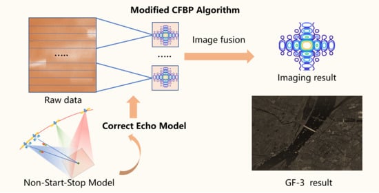
A Modified Cartesian Factorized Backprojection Algorithm Integrating with Non-Start-Stop Model for High Resolution SAR Imaging

Abstract

High resolution synthetic aperture radar (SAR) imaging has extensive application value especially in military reconnaissance and disaster monitoring. The motion of the satellite during the transmission and reception of the signal introduces notable errors in the high resolution SAR spotlight mode, which will lead to a defocused SAR image if not handled. To address this problem, an accurate correct echo model based on non-start-stop model is derived to describe the property of the SAR signal in the paper. Then, in the imaging processing, an azimuth-time-varying range frequency modulation rate is used for range compression. The range history and compensation phase are also derived based on the correct echo model. Then, combining the correct echo model and Cartesian factorized backprojection (CFBP) algorithm, a modified CFBP algorithm is proposed for SAR imaging to improve the accuracy and efficiency of processing. Besides, the influence of residual error due to mismatch is analyzed in detail. In the end, the simulation experiment and Gaofen-3 (GF-3) data experiment are carried out to demonstrate the feasibility of the proposed algorithm.

1. Introduction

Synthetic aperture radar (SAR), which can provide remote sensing images during the day and night regardless of weather conditions, plays an important role in Earth and planetary observation [1,2,3]. In recent years, high resolution SAR imaging attracts growing interest due to its wide applications especially in military reconnaissance and disaster monitoring [4,5,6,7,8,9,10]. Several spaceborne SAR systems have the ability of submeter imaging. For example, the COSMO-SkyMed SAR can achieve a high azimuth resolution better than 0.9 m [6], while TerraSAR-X can achieve 0.16 m azimuth resolution [7]. In addition, the Gaofen-3 (GF-3) satellite, a C-band multi-polarization SAR of China launched in 2016, can achieve 0.4 m azimuth resolution [5,10]. The realization of high resolution SAR imaging not only puts forward new requirements to the hardware of SAR system but also poses new challenges to the imaging algorithm.

In the high resolution spotlight mode, the satellite steers its antenna beam to continuously illuminate the same area of interest. As a result, the raw signal azimuth bandwidth is larger than pulse repetition frequency (PRF) [11], which increases the difficulty of imaging processing compared with the stripmap mode. A standard approach employed when processing the SAR data is based on the start-stop approximation, with the assumption that the radar transmits and receives the signal at the same position [12]. Although it has been widely used in SAR echo model, it is no longer applicable in high resolution spotlight case [7]. Therefore, the non-start-stop model should be used in imaging processing [13]. Additionally, due to the long trajectory, the error introduced by curved orbit should also be corrected [6]. Topography dependence and atmospheric effects should be considered [7,14], which further increases the complexity of imaging processing.

In order to solve the problems mentioned above, numerous algorithms have been proposed for high resolution SAR imaging. The full-aperture algorithm and subaperture algorithm are two typical frequency domain algorithms. The two-step processing approach [11], integrated with the efficiency of SPECAN algorithms and the precision of stripmap focusing techniques, is a typical full aperture approach and has been further studied in [15]. The subaperture algorithm first divides the raw data into subapertures in the azimuth time domain and the high-resolution is obtained by synthesizing the coarse resolution images of each subaperture [7,16]. The subaperture algorithm solves the curved orbit problem by motion compensation. However, there are residual errors due to the variance of echo signal property along range and azimuth directions. Besides, there are some inconveniences for frequency domain algorithms to adapt to the topography variance in the ground. The time domain algorithm is available for different SAR configurations and the imaging result on the ground can be obtained directly by time domain algorithm [14,17,18]. The backprojection algorithm (BPA), a typical time domain algorithm, has been widely used in SAR imaging [19,20]. The disadvantage of BPA is its high computational burden. There are two strategies for improving the efficiency of BPA. One strategy is using parallel computing tool, for example, GPU. In recent years, the development of GPU has made significant progress. The parallel BPA based on the GPU has been attracting more and more attention and there is great progress in the acceleration of the BPA [19,20,21]. Another strategy is developing the fast algorithms. Numerous fast algorithms of BPA have been developed in the last few decades [22,23,24,25,26,27,28,29]. The fast factorized BP (FFBP) algorithm, which splits long synthetic aperture into short subapertures to generate coarse resolution images and then fuses coarse resolution images to form the final image via interpolation, is an effective algorithm to reduce the computational burden [23,30]. However, the massive interpolations limit the efficiency and introduce errors that result in artifacts in the final image. The accelerating fast BP (AFBP) algorithm is proposed for the high-resolution SAR imaging [29]. The AFBP algorithm only contains two stages: subimage formation in unified polar coordinate and subimage fusion in the 2-D wavenumber domain, which can improve efficiency compared with FFBP algorithm [29]. The Cartesian factorized BP (CFBP) algorithm is proposed in [25,31] and has been further studied in [26,32,33]. Two spectrum compressing filters are applied in CFBP algorithm, which can decrease the cross-range Nyquist sampling rate (NSR) enormously, therefore reducing the computational burden. In addition, during image combination, interpolation can be easily achieved by zero-padding in the azimuth frequency domain, leading to a substantial improvement on both the accuracy and the efficiency [33].

In this paper, a modified CFBP algorithm is proposed for high resolution spotlight SAR imaging. Since the traditional echo model is derived based on start-stop approximation, there will be intolerable error in high resolution case, which will cause defocusing of the target. In order to solve this problem, an accurate correct echo model is firstly derived. The non-start-stop model and curved orbit are all taken into consideration in the correct model. Then, based on the correct echo mode, an azimuth-time-varying range frequency modulation (FM) rate is used for range compression. The position of the target after range compression is also derived. In addition, the azimuth phase in the correct echo model is also changed compared with the traditional echo mode. A discussion for residual phase error after range compression is given, which shows that the error is small and has little effect on the focusing of the target.

The correct echo model and CFBP algorithm are combined, which can integrate the non-start-stop model and curved orbit, further improving the imaging processing efficiency. The algorithm can be divided into seven steps: aperture division and subimage formation, first compression filter step, second compression filter step, azimuth sampling, second compression filter recovery step, first compression filter recovery step, coherent accumulation of subimage and recursion. After recursion step, the final image with full resolution can be obtained. The detailed processing flow of the proposed algorithm is introduced in detail in the paper. In addition, the simulation experiment with 0.07 m azimuth resolution and 0.21 m ground range resolution is performed to show the performance of the proposed algorithm. GF-3 data with 8.58 s synthetic aperture time are also performed to verify the effectiveness of the proposed algorithm. The azimuth-time-varying FM rates of targets in the center and edge of the scene are calculated for comparison. The focusing quality of targets is also evaluated.

The rest of this paper is organized as follows. The echo model of SAR is introduced in Section 2. The comparison of correct echo model and traditional echo model is discussed. The modified CFBP algorithm is also described in detail and the processing flow of the proposed algorithm is presented. In Section 3, the validity of the proposed method is confirmed by simulation experiment and GF-3 data experiment. In Section 4, a discussion is given to show the performance and advantages of the proposed algorithm. Section 5 concludes this paper.

2. Materials and Methods

In this section, the traditional echo model and proposed correct echo model are introduced in detail, followed by a comparison between the two models. Then, the modified CFBP algorithm is described and the residual error in the modified CFBP algorithm is analyzed. In addition, the processing flow of the algorithm is presented.

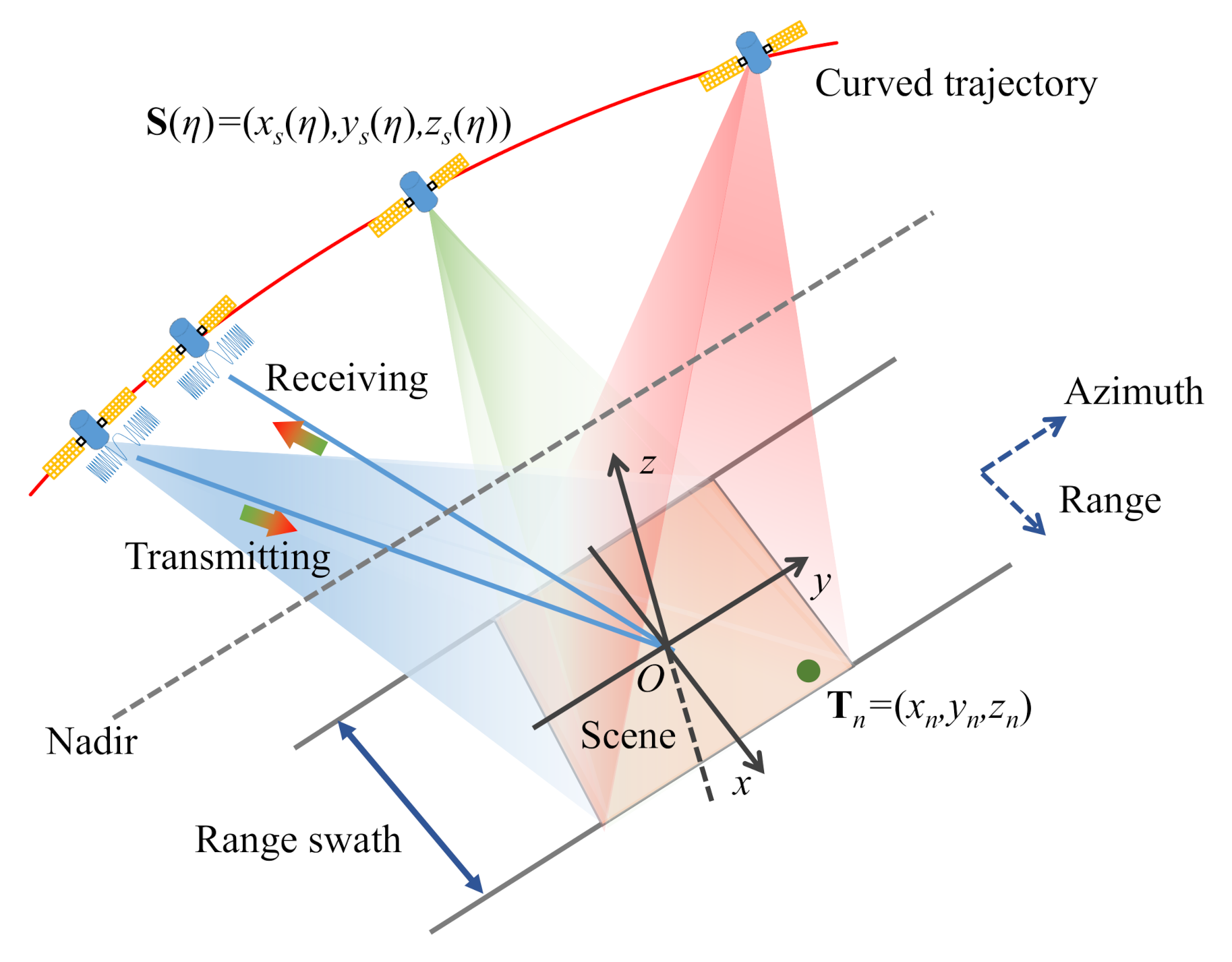
2.1. Echo Model of SAR

In this subsection, the traditional echo model is introduced first. Then, the correct echo model based on the non-start-stop model is derived in detail.

2.1.1. Traditional Echo Model

In the spotlight mode, the beam of SAR system is steered to illuminate the common spot on the surface of Earth, as Figure 1 shows. In O-$xyz$ coordinate, original point O is located at the center of the scene. The x-axis is along the direction of mean velocity of the satellite and y-axis is along the ground range direction.

Figure 1. The geometry of spotlight mode with right looking.

Suppose the position of nth target is ${\mathbf{T}}_n=(x_n,y_n,z_n)$ and the satellite position is $\mathbf{S}\left(\eta \right)=(x_s\left(\eta \right),y_s\left(\eta \right),z_s\left(\eta \right))$ at azimuth time $\eta$. The start-stop approximation is widely used in conventional SAR algorithms. Under this approximation, range the history of SAR signal can be expressed as $R\left(\eta \right)=\parallel \mathbf{S}\left(\eta \right)-{\mathbf{T}}_n\parallel$, where $\parallel ·\parallel$ denotes the norm. The propagation delay ${\tau }_0\left(\eta \right)=2R\left(\eta \right)/c$ is a function of azimuth time $\eta$, where c denotes the speed of light. The echo model can be written as [34]

$$S_0(\tau ,\eta )=A_0{w}_r\left(\tau -{\tau }_0\left(\eta \right)\right)w_a\left(\eta \right)\exp \left\{j\pi K_r{\left(\tau -{\tau }_0\left(\eta \right)\right)}^2\right\}\exp \left\{-j2\pi f_0{\tau }_0\left(\eta \right)\right\}$$

(1)

where $A_0$ is a complex constant, $f_0$ is the carrier frequency, $K_r$ is the FM rate of the transmitted signal, $w_r$ is range envelope, and $w_a$ is azimuth envelope.

2.1.2. Problem

Although the start-stop approximation is widely used in SAR imaging processing, it will introduce intolerable errors in spaceborne high resolution case. As mentioned in [7], the start-stop approximation will introduce two effects, slow-time effects, and and fast-time effects. The error introduced by the slow-time effect will introduce an azimuth shift which will not influence the focusing of the target. In 2D frequency domain, the phase error introduced by fast-time effect can be expressed as [7]

$$error=2\pi \frac{f_a{f}_r}{K_r}$$

(2)

where $f_a$ is the azimuth frequency. $f_r$ is the range frequency with $-B_r/2\le f_r\le B_r/2$, where $B_r$ is the range bandwidth. In the edge of the 2D frequency domain (corresponding to the position where azimuth frequency and range frequency reach their maximum), the error can be given by

$$erro{r}_{edge}=2\pi \frac{f_{a,max}{f}_{r,max}}{K_r}=2\pi \frac{f_{a,max}{B}_r/2}{K_r}=\pi f_{a,max}{T}_r$$

(3)

where $f_{a,max}$ is the maximum of azimuth frequency, $f_{r,max}$ is the maximum of range frequency, and $T_r$ is the pulse width. For a SAR data with 600 MHz range bandwidth and 20,000 Hz azimuth bandwidth, the phase of error $H(f_a,f_r)$ can be seen in Figure 2a (suppose the pulse width $T_r$ is 50 $\mathsf{\mu }$s and the corresponding $K_r$ is 1.2 $\times {10}^{13}$ Hz/s). The phase error $erro{r}_{edge}$ in the edge of the 2D frequency domain will reach 80 degrees, which should be corrected in the imaging processing. Furthermore, the change of $erro{r}_{edge}$ varied with $T_r$ and $f_{a,max}$ is shown in Figure 2b. As we can see, the phase error $erro{r}_{edge}$ increases with the increase of $T_r$ and $f_{a,max}$. In high resolution case, $erro{r}_{edge}$ is large, thus, the start-stop approximation is no longer applicable.

Figure 2. The phase error introduced by fast-time effect. (a) The error in 2D frequency domain with 600 MHz range bandwidth and 20,000 Hz azimuth bandwidth (b) the edge error $erro{r}_{edge}$ varies with pulse width $T_r$ and the maximum of azimuth frequency $f_{a,max}$.

2.1.3. Correct Echo Model

As mentioned above, in the high resolution spotlight mode of SAR, the motion of the satellite during the transmission and reception of the signal will introduce intolerable error [7,35]. Therefore, the non-start-stop model should be used in the high resolution spotlight mode of SAR. The propagation delay ${\tau }_d$ in non-start-stop model is a function of the fast time $\tau$ and the azimuth time $\eta$. A refined model that takes this motion into account is defined as [35,36]

$${\tau }_d=\frac{1}{c}\left(R_T(\eta +{\tau }_s)+R_R(\eta +\tau )\right)$$

(4)

where $(\eta +{\tau }_s)$ denotes the transmitting time of the radar signal, $R_T(\eta +{\tau }_s)=\parallel \mathbf{S}(\eta +{\tau }_s)-{\mathbf{T}}_n\parallel$ is the transmitting distance. $R_R(\eta +\tau )=\parallel \mathbf{S}(\eta +\tau )-{\mathbf{T}}_n\parallel$ is the receiving distance. ${\tau }_s$ is related to $\tau$ by the following equation [36]

$$\tau ={\tau }_s+{\tau }_d$$

(5)

Suppose $\mathbf{V}\left(\eta \right)=(v_x\left(\eta \right),v_y\left(\eta \right),v_z\left(\eta \right))$ denotes the velocity of the satellite at azimuth time $\eta$. Assume $\mathbf{V}\left(\eta \right)$ is invariant during the transmission and reception of the signal. Therefore, Equation (4) can be expressed as

$$\begin{array}{}c{\tau }_d=\parallel \mathbf{S}\left(\eta \right)+(\tau -{\tau }_d)\mathbf{V}\left(\eta \right)-{\mathbf{T}}_n\parallel +\parallel \mathbf{S}\left(\eta \right)+\tau \mathbf{V}\left(\eta \right)-{\mathbf{T}}_n\parallel \approx 2R\left(\eta \right)+(2\tau -{\tau }_d)\parallel \mathbf{V}\left(\eta \right)\parallel cos{\theta }_n\end{array}$$

(6)

where $\theta$ is given as follows

$${\theta }_n=arccos\left(\frac{\mathbf{V}\left(\eta \right)·(\mathbf{S}\left(\eta \right)-{\mathbf{T}}_n)}{\parallel \mathbf{V}\parallel \parallel \mathbf{S}\left(\eta \right)-{\mathbf{T}}_n)\parallel }\right)$$

(7)

Therefore, the propagation delay ${\tau }_d$ can be derived as [17]

$${\tau }_d=\frac{2R\left(\eta \right)+2\tau \parallel \mathbf{V}\left(\eta \right)\parallel cos{\theta }_n}{c+\parallel \mathbf{V}\left(\eta \right)\parallel cos{\theta }_n}={\tau }_{d,n}\left(\eta \right)+{\alpha }_n\left(\eta \right)\tau$$

(8)

where

$$\begin{array}{c}\hfill {\tau }_{d,n}\left(\eta \right)=\frac{2R\left(\eta \right)}{c+\parallel \mathbf{V}\left(\eta \right)\parallel cos{\theta }_n}\end{array}$$

(9)

$$\begin{array}{c}\hfill {\alpha }_n\left(\eta \right)=\frac{2\parallel \mathbf{V}\left(\eta \right)\parallel cos{\theta }_n}{c+\parallel \mathbf{V}\left(\eta \right)\parallel cos{\theta }_n}\end{array}$$

(10)

As a result, the correct echo model can be expressed as follows

$$S_0(\tau ,\eta )=A_0{w}_r\left(\tau -{\tau }_d\right)w_a\left(\eta \right)\exp \left\{-j2\pi f_0{\tau }_d\right\}\exp \left\{j\pi K{\left(\tau -{\tau }_d\right)}^2\right\}$$

(11)

For simplicity, $A_0$, $w_r\left(\tau \right)$ and $w_a\left(\eta \right)$ in Equation (11) are ignored in the subsequent analysis. Thus, Equation (11) can be derived as

$$\begin{array}{ll}{S}_0(\tau ,\eta )& =\exp \left\{j\pi K_r{(1-{\alpha }_n\left(\eta \right))}^2{\left(\tau -\frac{{\tau }_{d,n}\left(\eta \right)}{1-{\alpha }_n\left(\eta \right)}\right)}^2\right\}\exp \left\{-j2\pi f_0({\tau }_{d,n}\left(\eta \right)+{\alpha }_n\left(\eta \right)\tau )\right\}\\ & =\exp \left\{j\pi K_n\left(\eta \right){\left(\tau -\left(\frac{{\tau }_{d,n}\left(\eta \right)}{1-{\alpha }_n\left(\eta \right)}+\frac{f_0{\alpha }_n\left(\eta \right)}{K_n\left(\eta \right)}\right)\right)}^2\right\}\exp \left\{-j2\pi f_0\frac{{\tau }_{d,n}\left(\eta \right)}{1-{\alpha }_n\left(\eta \right)}-j\pi f_0^2\frac{{\alpha }_n^2\left(\eta \right)}{K_n\left(\eta \right)}\right\}\end{array}$$

(12)

where

$$K_n\left(\eta \right)=K_r{(1-{\alpha }_n\left(\eta \right))}^2$$

(13)

$K_n\left(\eta \right)$ denotes the range FM rate which is varying with azimuth time $\eta$.

2.1.4. Comparison between the Traditional Echo Model and the Correct Echo Model

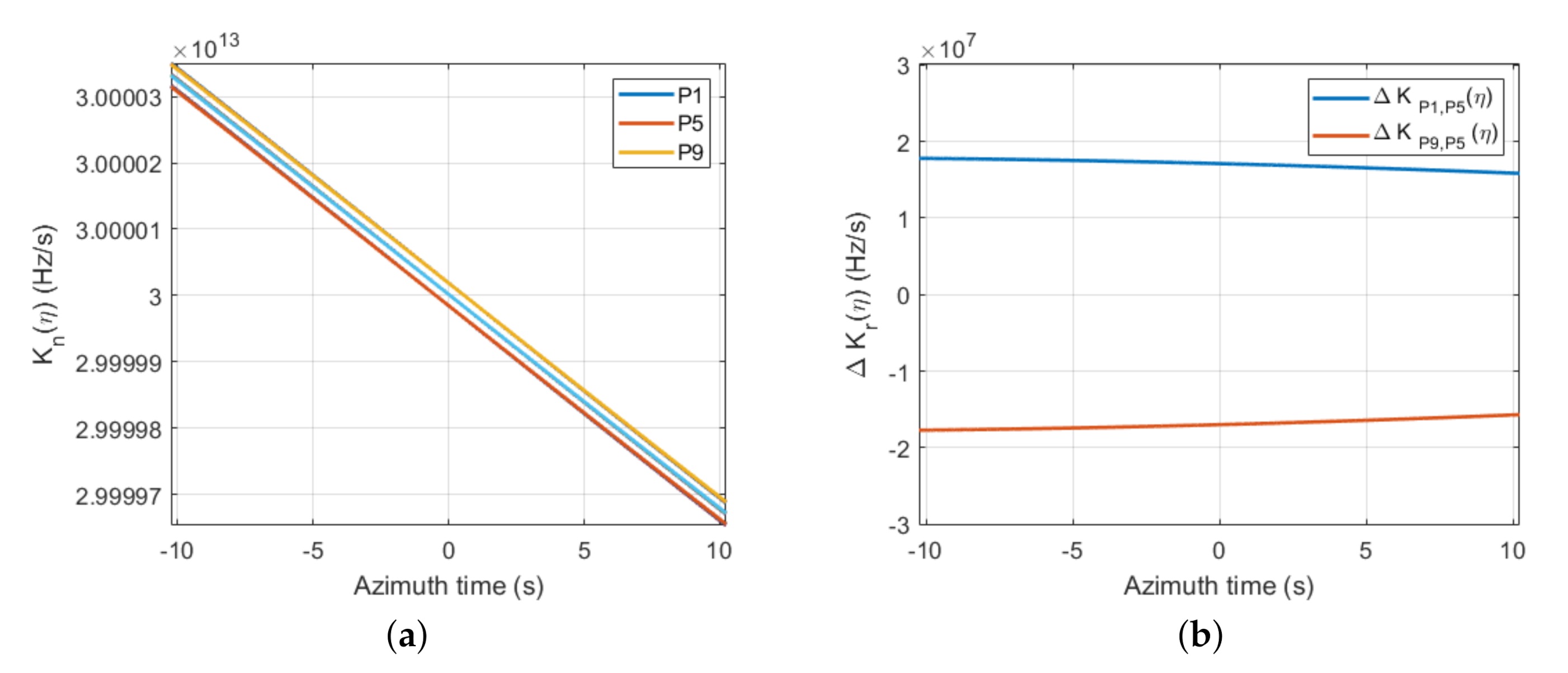
As shown in Table 1, the difference between the traditional echo model and the correct echo model can be summarized as follows:

Table 1. The comparison between the traditional echo model and the correct echo model

Model	Traditional Echo Model	Correct Echo Model
Range FM rate	$K_r$	$K_r\left(\eta \right)$
Target position in range line	${\tau }_0\left(\eta \right)$	$\frac{{\tau }_{d,n}\left(\eta \right)}{1-{\alpha }_n\left(\eta \right)}+\frac{f_0{\alpha }_n\left(\eta \right)}{K_n\left(\eta \right)}$
Azimuth compensation phase	$2\pi f_0{\tau }_0\left(\eta \right)$	$2\pi f_0\frac{{\tau }_{d,n}\left(\eta \right)}{1-{\alpha }_n\left(\eta \right)}+\pi f_0^2\frac{{\alpha }_n^2\left(\eta \right)}{K_n\left(\eta \right)}$

• A new range FM rate expression. $K_n\left(\eta \right)$ can be regarded as an azimuth-time-varying FM rate in the correct echo model, while the range FM rate $K_r$ is constant in the traditional echo model.
• The position of the target after range compression is shifted. In the traditional echo model, the position of the target after range compression is ${\tau }_0\left(\eta \right)$. However, in the correct echo model, the peak position is $\frac{{\tau }_{d,n}\left(\eta \right)}{1-{\alpha }_n\left(\eta \right)}+\frac{f_0{\alpha }_n\left(\eta \right)}{K_n\left(\eta \right)}$.
• The azimuth phase is different. In the traditional echo model, the azimuth phase is $2\pi f_0{\tau }_0\left(\eta \right)$. However, in the correct echo model, the azimuth phase is $2\pi f_0\frac{{\tau }_{d,n}\left(\eta \right)}{1-{\alpha }_n\left(\eta \right)}+\pi f_0^2\frac{{\alpha }_n^2\left(\eta \right)}{K_n\left(\eta \right)}$.

2.2. Modified Cartesian Factorized Backprojection Algorithm

In this section, the proposed modified CFBP algorithm is introduced in detail. An azimuth-time varying range FM rate is used for range compression. The residual error due to mismatch is also analyzed in detail. Then, the range history and compensation phase are derived for imaging processing. Finally, the processing flow chart of the proposed algorithm is presented.

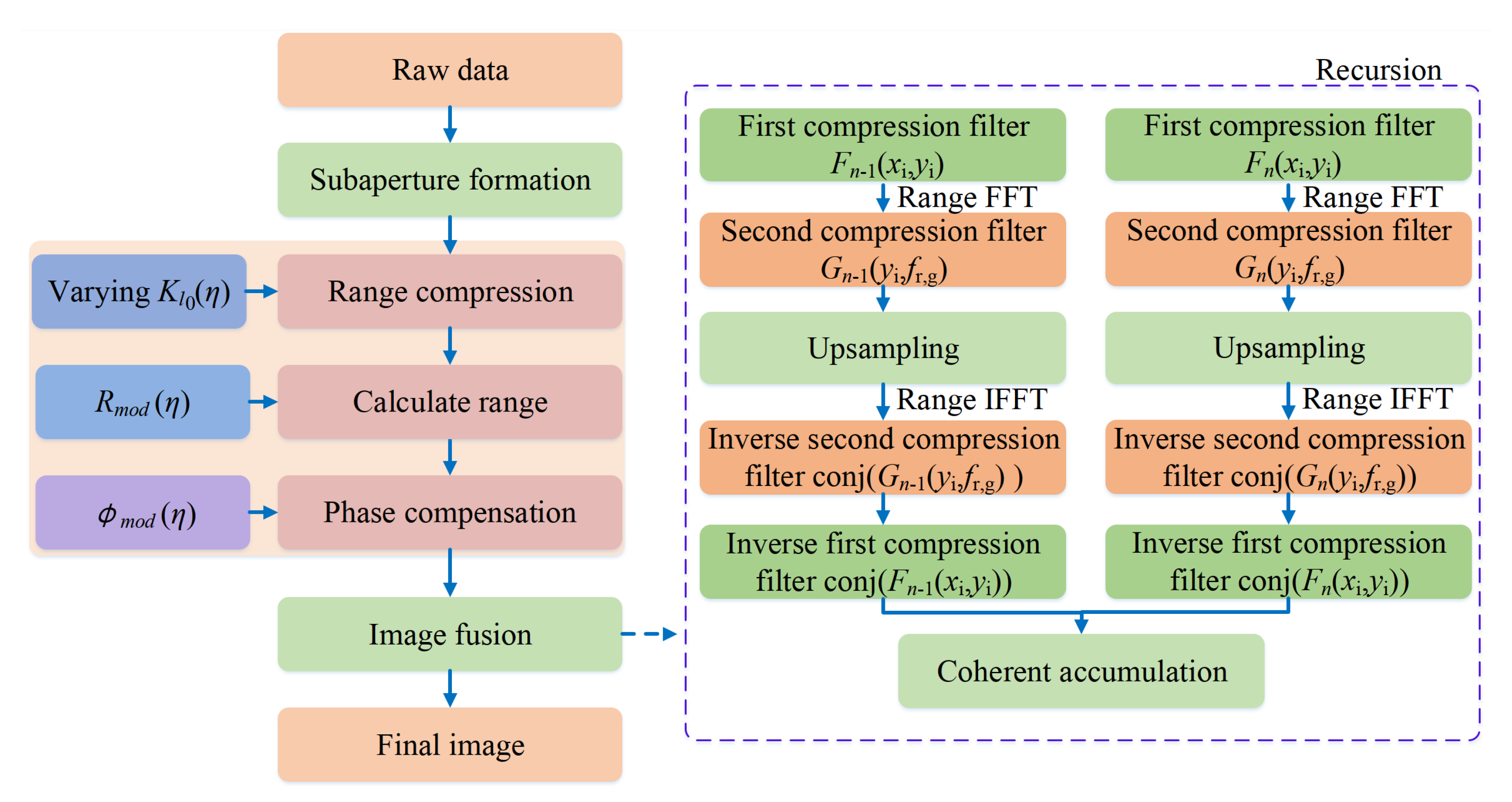
2.2.1. Processing Flow of the Modified CFBP Algorithm

In the first step of the imaging processing, an azimuth-time-varying FM rate $K_n\left(\eta \right)$ is used for range compression. However, it can be seen from Equation (13) that $K_n\left(\eta \right)$ is dependent on the relative position between the target and SAR platform. As a result, $K_n\left(\eta \right)$ is different for different targets.

In general, in order to improve the efficiency of processing, the target ${\mathbf{T}}_0$ in the center of the scene is selected as the reference point. Therefore, $K_0\left(\eta \right)$ calculated from the target ${\mathbf{T}}_0$ is used for range compression. Thus, the focusing quality of the target ${\mathbf{T}}_0$ is the best in the scene. The residual error of other targets in the scene introduced by the range compression mismatch should be analyzed. The detailed analysis can be seen in the next subsection.

After range compression, the signal can be expressed as follows

$$\begin{array}{cc}\hfill S_0(\tau ,\eta )& =\mathrm{sinc}\left\{B_r{\left(\tau -\left(\frac{{\tau }_{d,n}\left(\eta \right)}{1-{\alpha }_n\left(\eta \right)}+\frac{f_0{\alpha }_n\left(\eta \right)}{K_n\left(\eta \right)}\right)\right)}^2\right\}\exp \left\{-j2\pi f_0\frac{{\tau }_{d,n}\left(\eta \right)}{1-{\alpha }_n\left(\eta \right)}-j\pi f_0^2\frac{{\alpha }_n^2\left(\eta \right)}{K_n\left(\eta \right)}\right\}\hfill \end{array}$$

(14)

where $B_r$ is the range frequency bandwidth. Transform the Equation (14) into the range frequency domain

$$\begin{array}{}{S}_0(f,\eta )=\mathrm{rect}\left(\frac{f_r}{B_r}\right)\exp \left\{-j2\pi f_r{\left(\frac{{\tau }_{d,n}\left(\eta \right)}{1-{\alpha }_n\left(\eta \right)}+\frac{f_0{\alpha }_n\left(\eta \right)}{K_n\left(\eta \right)}\right)}^2\right\}\exp \left\{-j2\pi f_0\frac{{\tau }_{d,n}\left(\eta \right)}{1-{\alpha }_n\left(\eta \right)}-j\pi f_0^2\frac{{\alpha }_n^2\left(\eta \right)}{K_n\left(\eta \right)}\right\}\end{array}$$

(15)

In first processing step of CFBP algorithm, the synthetic aperture is split into N subapertures. The impulse response function (IRF) at position $(x_i,y_i,z_i)$ generated from nth subaperture can be written as

$$I_n(x_i,y_i)={\int }_{{\eta }_{n,begin}}^{{\eta }_{n,end}}{S}_0(\tau ,\eta )\exp \left\{j2\pi f_0\frac{{\tau }_{d,n}\left(\eta \right)}{1-{\alpha }_n\left(\eta \right)}+j\pi f_0^2\frac{{\alpha }_n^2\left(\eta \right)}{K_n\left(\eta \right)}\right\}d\eta$$

(16)

where ${\eta }_{n,begin}$ and ${\eta }_{n,end}$ denotes the start and the end times of the nth subaperture.

To decrease the NSR of subimage, two spectrum compression filters of nth subaperture are used in CFBP algorithm, which can be expressed as follows [31,33]

$$F_n(x_i,y_i)=\exp \left(-\frac{4\pi f_0}{c}\sqrt{{\left(X_s\left({\eta }_{n,cen}\right)-x_i\right)}^2+{\left(Y_s\left({\eta }_{n,cen}\right)-y_i\right)}^2+{\left(Z_s\left({\eta }_{n,cen}\right)\right)}^2}\right)$$

(17)

$$G_n(y_i,f_{r,g})=\exp \left(-j\frac{4\pi f_{r,g}}{c}\sqrt{{\left(X_s\left({\eta }_{n,cen}\right)-x_{i,cen}\right)}^2+{\left(Y_s\left({\eta }_{n,cen}\right)-y_i\right)}^2+{\left(Z_s\left({\eta }_{n,cen}\right)\right)}^2}\right)$$

(18)

where $\left(X_s\left({\eta }_{n,cen}\right),Y_s\left({\eta }_{n,cen}\right),Z_s\left({\eta }_{n,cen}\right)\right)$ denotes the aperture center position of nth subaperture. $x_{i,cen}$ is the center value of $x_i$ in the scene. $f_{r,g}$ is the subimage range frequency and its relationship with $f_r$ can be expressed as

$$f_{r,g}=f_r\frac{1}{sin\left(\theta \right)}=f_r\frac{\sqrt{{\left(X_s\left({\eta }_{cen}\right)\right)}^2+{\left(Y_s\left({\eta }_{cen}\right)\right)}^2+{\left(Z_s\left({\eta }_{cen}\right)\right)}^2}}{\sqrt{{\left(X_s\left({\eta }_{cen}\right)\right)}^2+{\left(Y_s\left({\eta }_{cen}\right)\right)}^2}}$$

(19)

where $\theta$ is the incidence angle. $\left(X_s\left({\eta }_{cen}\right),Y_s\left({\eta }_{cen}\right),Z_s\left({\eta }_{cen}\right)\right)$ denotes the aperture center position of whole subaperture. The first spectrum compression filter $F_n(x_i,y_i)$ is used to compress the 2-D wavenumber support region [33]. However, the azimuth bandwidth may still large due to the varying range frequency. Therefore, the second spectrum compression filter is performed in the range frequency domain to correct the azimuth spectrum expand [33]. The detailed derivation can be seen in [33]. After operating with two spectrum compression filters, the azimuth bandwidth of the subperture image is reduced, thus, a small NSR is enough for subaperture imaging. As a result, the computational burden is reduced greatly while operating backprojection algorithm in subaperture for subimage formation. The following step is upsampling by zero-padding in 2D frequency domain to get a high NSR of the subimage. After decompressed by two spectrum compression filters, two subimages can be added up to get a higher resolution image. After step-and-repeat operation, the final image with full resolution can be obtained.

In the imaging processing, another problem that needs to be considered is how to determine the number of subaperture. In [25], the formula of length of subaperture l is given as follows

$$l\ge \frac{B_r\beta cos\left(\beta /2\right)}{4f_0(\gamma -1-\frac{{\beta }^2}{4})}{\left|x_i\right|}_{R}sin\left(\theta \right)$$

(20)

where $\beta$ represents the azimuth width of the beam, $\gamma$ represents the azimuth oversampling ratio and $|x_i{|}_R$ is the ground range width of a subscene. As stated in [25], the whole scene can be divided along the range direction according to Equation (20) in spotlight mode of SAR system.

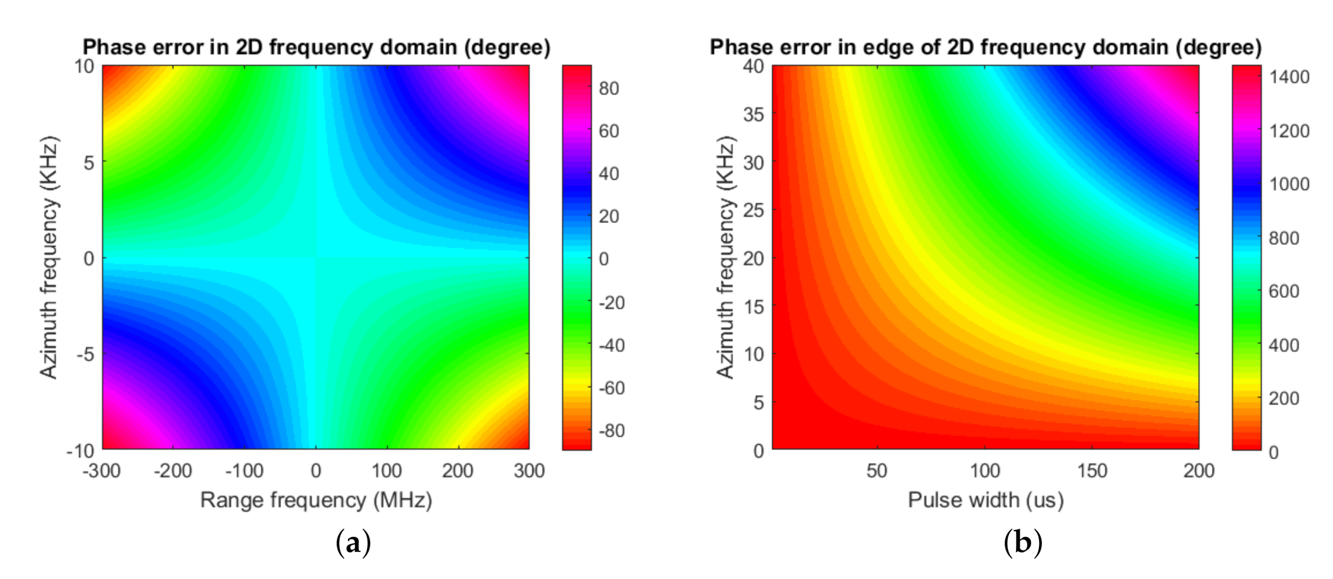
2.2.2. Derivation of the Error Due to Mismatch

The range FM rate $K_n\left(\eta \right)$ is varying with azimuth time $\eta$ in the correct echo model. Therefore, in the first step of the imaging processing, an azimuth-time-varying FM rate $K_n\left(\eta \right)$ is used for range compression. However, it can be seen from Equation (13) that $K_n\left(\eta \right)$ is dependent on the relative position between the target and SAR platform. As a result, $K_n\left(\eta \right)$ is different for different targets.

In general, in order to improve the efficiency of processing, the target ${\mathbf{T}}_0$ in the center of the scene is selected as the reference point. Therefore, $K_0\left(\eta \right)$ calculated from the target ${\mathbf{T}}_0$ is used for range compression. Thus, the focusing quality of the target ${\mathbf{T}}_0$ is the best in the scene. The residual error of other targets in the scene introduced by the range compression mismatch should be analyzed.

The range FM rate difference $\Delta K_{n,0}\left(\eta \right)$ between the target ${\mathbf{T}}_n$ and ${\mathbf{T}}_0$ can be written as

$$\Delta K_{n,0}\left(\eta \right)=K_n\left(\eta \right)-K_0\left(\eta \right)=K({(1-{\alpha }_n\left(\eta \right))}^2-{(1-{\alpha }_0\left(\eta \right))}^2)$$

(21)

$\Delta K_{n,0}\left(\eta \right)$ causes a filter mismatch in range direction, which broadens the impulse response width (IRW) and increases the size of sidelobes [34]. The quadratic phase error ($\mathrm{QPE}$), which characterizes the broadening of range signal after range compression, is defined as follows [34]

$$\mathrm{QPE}=\pi \Delta K_{n,0}\left(\eta \right){\left(\frac{T_r}{2}\right)}^2$$

(22)

where $T_r$ is the pulse width of range signal. The phase error $\Delta \varphi$ in the peak position caused by $\Delta K_0\left(\eta \right)$ can be expressed as follows [34]

$$\Delta \varphi =-\frac{1}{3}\mathrm{QPE}=-\frac{\pi }{3}\Delta K_{n,0}\left(\eta \right){\left(\frac{T_r}{2}\right)}^2$$

(23)

In the imaging processing, if the IRW broadening and phase error $\Delta \varphi$ are at a tolerable level, $K_0\left(\eta \right)$ calculated from the target ${\mathbf{T}}_0$ in the center of the scene can be used for range compression. However, if the IRW broadening and phase error $\Delta \varphi$ are large, which would degrade the focusing quality seriously, $K_0\left(\eta \right)$ used for range compression is no longer applicable. From the simulation experiment in Section 3, we can see that the IRW broadening and phase error are small which will not influence the focus of edge targets. In addition, the phase error due to mismatch can be compensated in the processing, which can further improve the accuracy of phase in the final image.

2.2.3. Algorithm Steps

Based on the former investigation, the algorithm steps are summarized as follows for the convenience of implementation. The processing flow can also be seen in Figure 3.

Figure 3. The processing flow of the proposed algorithm.

Step 1 

Aperture division and subimage formation. The BPA is used for subimage formation.

1 

Range compression by a varying frequency modulation rate $K_0\left(\eta \right)$.

2 

The peak position in the compressed signal for target ${\mathbf{T}}_n$ is $R_{mod}\left(\eta \right)=\frac{{\tau }_{d,n}\left(\eta \right)}{1-{\alpha }_n\left(\eta \right)}+\frac{f_0{\alpha }_n\left(\eta \right)}{K_n\left(\eta \right)}$.

3 

The peak position in the compressed signal for target ${\mathbf{T}}_n$ is $R_{mod}\left(\eta \right)=\frac{{\tau }_{d,n}\left(\eta \right)}{1-{\alpha }_n\left(\eta \right)}+\frac{f_0{\alpha }_n\left(\eta \right)}{K_n\left(\eta \right)}$. The compensation phase is ${\varphi }_{mod}\left(\eta \right)=2\pi f_0\frac{{\tau }_{d,n}\left(\eta \right)}{1-{\alpha }_n\left(\eta \right)}+\pi f_0^2\frac{{\alpha }_{l_b}^2\left(\eta \right)}{K_n\left(\eta \right)}+\Delta {\varphi }_{com}$, where $\Delta {\varphi }_{com}=\frac{\pi }{3}\Delta K_{n,0}\left(\eta \right){\left(\frac{T_r}{2}\right)}^2$ denotes the residual compensation phase due to mismatch.

Step 2 

First compression filter step. It is operated in 2D time domain.

Step 3 

Second compression filter step. It is operated in ground range frequency domain.

Step 4 

Azimuth upsampling. Azimuth upsampling is operated in the azimuth frequency domain by using zero-padding method.

Step 5 

Second compression filter recovery step. Multiply the conjugated second compression filter in the corresponding domain.

Step 6 

First compression filter recovery step. Multiply the conjugated first compression filter in the corresponding domain.

Step 7 

Coherent accumulation of subimage. Add up the subimage after upsampling for coherent accumulation.

Step 8 

Recursion. Repeat the step3 to step8 until the final image with full resolution is obtained.

It should be noted that in the processing of phase compensation in step2, the phase error $\Delta {\varphi }_{com}$ introduced by range FM rate mismatch is also compensated, which improves the phase accuracy of the imaging result. As a result, the error of IRW broadening exists in the final image. From the simulation analysis in Section 3, it can be seen that the IRW boarding error is small which will cause negligible error in the final image.

3. Results

To show the effectiveness of the proposed algorithm, the simulation experiment and GF-3 data experiment are performed in this section. The results are compared with the traditional echo model. The azimuth-time-varying FM rates of different targets in the scene are calculated for comparison. In addition, the corresponding phase error is demonstrated to analyze its influence on the focusing of the target.

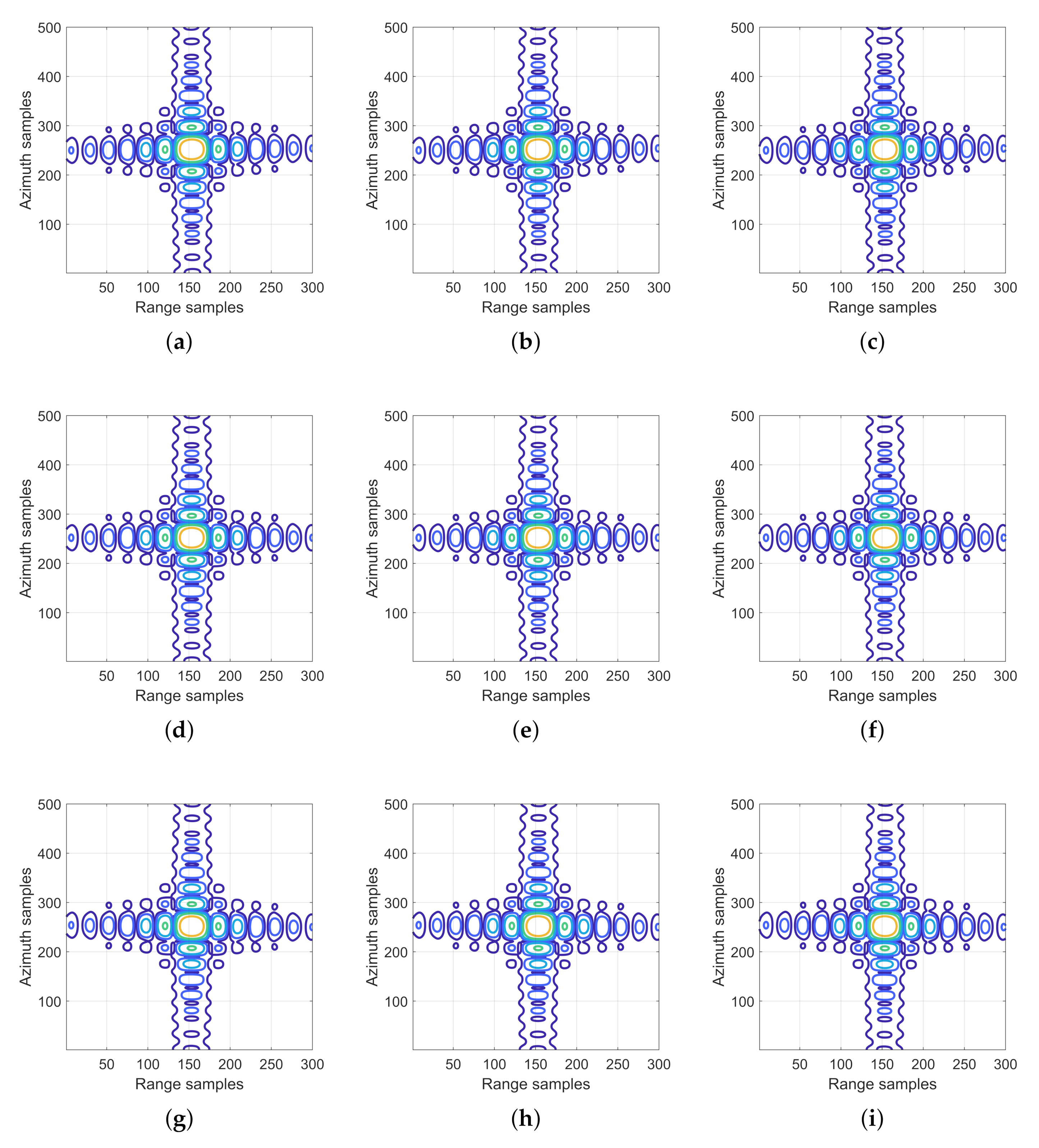
3.1. Simulation Experiment

In this subsection, the simulation experiments are carried out to validate the proposed algorithm. The satellite orbit parameters in Table 2 are used for simulation. The height of the satellite is 600 km. The orbit eccentricity is 0.0011. The parameters of the SAR system can be seen in Table 3. The synthetic aperture time is 20.47 s. Therefore, a resolution higher than 0.1 m in azimuth direction can be reached. The pulse width is 40 $\mathsf{\mu }$s. The motion of the platform between transmitting and receiving signals cannot be ignored due to the large pulse width. The spotlight mode SAR echo data is simulated with a 3 × 3 point target array being arranged in the simulation scene, which can be seen in Figure 4. The SAR echo is obtained by using the iteration method proposed in [13], which can simulate the continuous motion of the satellite.

Table 2. Parameters of Satellite Orbit in Simulation Experiment

Parameter	Value
Platform Height	600 km
Eccentricity	0.0011
Inclination	97.44 degrees
Semimajor axis	6971 km
Argument of perigee	78 degrees
Ascending node	80 degrees
Incidence angle	33.23 degrees

Table 3. Parameters of SAR System in Simulation Experiment

Parameter	Value
Carrier frequency	9.6 GHz
Pulse width	40 $\mathsf{\mu }$s
Range bandwidth	1.2 GHz
Range sampling frequency	1.4 GHz
Synthetic aperture time	20.47 s
PRF	6000 Hz
Scene extent	8 km × 8 km

Figure 4. The point target array in simulation experiment.

In the first step, the azimuth-time-varying range FM rates of target $P1$, $P5$ and $P9$ are calculated, which are shown in Figure 5a. Assume $\Delta K_{P1,P5}\left(\eta \right)$ denotes the range FM rate difference between target P1 and target P5, and $\Delta K_{P9,P5}\left(\eta \right)$ denotes the range FM rate difference between target P9 and target P5. $\Delta K_{P1,P5}\left(\eta \right)$ and $\Delta K_{P9,P5}\left(\eta \right)$ are shown in Figure 5a. If the range FM rate of P5 is used for range compression, the corresponding phase error of P1 and P9 can be written as

$$\begin{array}{cc}\hfill \Delta {\varphi }_{P1}& =-\frac{\pi }{3}\Delta K_{P1,P5}\left(\eta \right){\left(\frac{T_r}{2}\right)}^2\hfill \end{array}$$

(24)

$$\begin{array}{cc}\hfill \Delta {\varphi }_{P9}& =-\frac{\pi }{3}\Delta K_{P9,P5}\left(\eta \right){\left(\frac{T_r}{2}\right)}^2\hfill \end{array}$$

(25)

Figure 5. (a) The azimuth-time varying $K_n\left(\eta \right)$ of targets P1, P5 and P9. (b) $\Delta K_{P1,P5}\left(\eta \right)$ and $\Delta K_{P9,P5}\left(\eta \right)$ versus azimuth time.

The change of $\Delta {\varphi }_{P1}$ and $\Delta {\varphi }_{P9}$ over azimuth time $\eta$ can be seen in Figure 6a. The maximum $\parallel \Delta {\varphi }_{P1}\parallel$ and $\parallel \Delta {\varphi }_{P9}\parallel$ are less than 0.5 degrees, thus, the residual error due to mismatch in the whole scene is small. In addition, the IRW broadening of targets $P1$ and $P9$ can be seen in Figure 6b. The value of IRW broadening is less than 0.06%, which indicates that the influence of mismatch is small and the mismatch can be ignored in the analysis.

Figure 6. (a) The phase error $\Delta {\varphi }_{P1}$ and $\Delta {\varphi }_{P9}$ versus azimuth time. (b) IRW broadening of target P1 and P9 versus azimuth time.

After processing with the proposed algorithm, the interpolated contour of points P1~P9 can be seen in Figure 7. In addition, quantitative results of the imaging quality for P1∼P9 are listed in Table 4, including the IRW, the peak sidelobe ratio (PSLR), and the integration sidelobe ratio (ISLR) in range and azimuth directions. It can be seen that all targets have a good focusing performance, which verifies the feasibility of the proposed algorithm. In contrast, when the traditional echo model is employed, the imaging result of target P5 is shown in Figure 8 and the quantitative result of target $P5$ is shown in Table 5. In addition, the range and azimuth profiles of $P5$ by using the start-stop model and the non-start-stop model are shown in Figure 9 and Figure 10 respectively. The IRWs of range and azimuth direction are 0.4889 m and 0.1279 m respectively, which are much higher than the theoretical values. Compared with Figure 7e, the point $P5$ in Figure 8b is seriously defocused, which proves that the start-stop approximation is no longer applicable in high resolution case. In addition, the computational times of the modified CFBP algorithm and traditional BPA are also compared. The computational time of modified CFBP algorithm is about 7% computational time of traditional BPA, which denotes that the modified CFBP algorithm has high efficiency.

Figure 7. Imaging results of targets P1~P9 (corresponding to (a–i)) by using the proposed algorithm.

Table 4. Evaluation of Imaging Quality in Simulation Experiment by Using the Proposed Algorithm.

Targets	Range			Azimuth
	IRW (m)	PSLR (dB)	ISLR (dB)	IRW (m)	PSLR (dB)	ISLR (dB)
P1	0.2037	−13.32	−10.38	0.0634	−13.28	−10.54
P2	0.2021	−13.32	−10.37	0.0636	−13.28	−10.54
P3	0.2007	−13.32	−10.37	0.0638	−13.28	−10.54
P4	0.2036	−13.32	−10.36	0.0634	−13.27	−10.54
P5	0.2021	−13.32	−10.36	0.0636	−13.27	−10.54
P6	0.2007	−13.31	−10.35	0.0638	−13.27	−10.54
P7	0.2036	−13.32	−10.38	0.0634	−13.28	−10.54
P8	0.2023	−13.32	−10.38	0.0636	−13.28	−10.54
P9	0.2007	−13.32	−10.37	0.0638	−13.27	−10.54

Figure 8. Imaging results of target (a) $P1$, (b) $P5$, and (c) $P9$ by using start-stop model.

Table 5. Evaluation of Imaging Quality of $P5$ in Simulation Experiment by Using the Start-Stop Model.

Target	Range			Azimuth
	IRW (m)	PSLR (dB)	ISLR (dB)	IRW (m)	PSLR (dB)	ISLR (dB)
P5	0.4889	−4.9765	−10.7928	0.1279	−4.3672	−5.7967

Figure 9. The profile of $P5$ by using the non-start-stop model. (a) Range profile; (b) Azimuth profile.

Figure 10. The profile of $P5$ by using the start-stop model. (a) Range profile; (b) Azimuth profile.

3.2. Real Data Experiment

In this subsection, SAR raw data of spotlight mode acquired from GF-3 satellite are used to verify the effectiveness of the proposed algorithm.

The parameters of the raw data can be seen in Table 6. The carrier frequency is 5.4 GHz. The range bandwidth of the raw data is 240 MHz. The pulse duration of transmitted signal is 45 $\mathsf{\mu }$s. Although the beam steering ability of GF-3 satellite is −1.9${}^{\circ }$ to 1.9${}^{\circ }$, the steering range of the spotlight mode raw data is from −1.78${}^{\circ }$ to 1.78${}^{\circ }$ in this experiment. The corresponding acquisition time is 8.58 s. The theoretical azimuth resolution and ground range resolutions are 0.396 m and 0.889 m, respectively.

Table 6. Main Parameters of GF-3 Raw Data in Spotlight Mode.

Parameter	Value
Carrier frequency	5.4 GHz
Azimuth steering range	±${1.78}^{\circ }$
Look angle	33.75${}^{\circ }$
Incidence angle	38.51${}^{\circ }$
Range bandwidth	240 MHz
Range sampling frequency	266.67 MHz
Pulse duration	45 $\mathsf{\mu }$s
PRF	3742.80 Hz
Acquisition time	8.58 s

In the processing of the raw data, the azimuth-time-varying FM rate is calculated for range compression. $K_0\left(\eta \right)$ of point target in the center of the scene is shown in Figure 11a. The standard FM rate $K_r$ is $5.33333\times {10}^{12}$ Hz/s. The ratio of $K_0\left(\eta \right)$ to $K_r$ is shown in Figure 11b. The maximum of the ratio is about 1.000003. By using the proposed algorithm, the imaging result of GF-3 spotlight data can be seen in Figure 12. For comparison, the imaging result of local area A based on start-stop model is shown in Figure 13a. Compared with image in Figure 13a, the image in Figure 13b has a better focusing quality. In addition, the contour of one target with high reflectivity in the scene is shown in Figure 14. It can be seen that based on the non-start-stop model, the target has a high focusing quality, which proves the effectiveness of the proposed algorithm.

Figure 11. (a) The azimuth-time-varying FM rate $K_0\left(\eta \right)$ of center target in GF-3 experiment. (b) The ratio of $K_0\left(\eta \right)$ to $K_r$.

Figure 12. The imaging result of GF-3 spotlight data.

Figure 13. The imaging result of local area A based on (a,c) start-stop model and (b,d) non-start-stop model.

Figure 14. The imaging result of point target based on (a) start-stop model and (b) non-start-stop model.

4. Discussion

Nowadays, the spaceborne SAR system is characterized by high resolution and swath coverage. The high resolution mode of SAR system brings new difficulties and challenges. In this paper, a modified CFBP algorithm integrating with non-start-stop model is proposed for high resolution SAR imaging. The simulation experiment with 0.21 m range resolution and 0.07 m azimuth resolution demonstrates that the proposed algorithm can achieve high focusing quality. The GF-3 spotlight mode with 0.889 m range resolution and 0.396 m azimuth resolution is also used to verify the effectiveness of proposed algorithm. Compared with the tradition echo model, the proposed correct echo model considers the motion of the satellite during the transmission and reception of the SAR signal. A new range FM rate is derived, which is varied with azimuth time. The position of the target after range compression and the azimuth phase are also derived. The proposed echo model can reflect the true motion of satellite; therefore, it has high accuracy and can be applied to high resolution SAR mode case. The CFBP algorithm proposed in [25,26,31,32,33] is an efficient algorithm. In order to improve the efficiency of imaging processing, the correct echo model and CFBP algorithm are combined. In addition, the residual error due to mismatch is also derived. The results show that the residual error is small which can be ignored in the analysis.

The advantages of the proposed algorithm are as follows. The curved orbit and non-start-stop mode are all considered in the correct echo model, therefore, it has high accuracy. The whole aperture is divided into subapertures and the final image is obtained by coherent combination of subimages, which can improve the efficiency. Although in the subimage formation, the BPA is used which may increase computational burden; however, this step can be done by using parallel computing tool which can greatly increase efficiency [19,24,37].

5. Conclusions

The high resolution spotlight mode of SAR plays an increasingly important role in remote sensing. In this paper, a modified CFBP algorithm integrating with non-start-stop model is proposed for very high resolution spotlight mode of SAR data processing. In the high resolution case, the start-stop model will introduce errors, which will cause the target to be defocused in the image. In addition, under the condition of long synthetic aperture time, the error introduced by curved orbit should also be considered, further increasing the difficulty of imaging processing.

In this paper, an accurate correct echo model is used to depict the SAR signal with high accuracy. The non-start-stop model and curved orbit are all considered in the correct echo model. Then, The correct echo model and CFBP algorithm are combined to improve the accuracy and efficiency of imaging processing. Based on the echo model, at first, an azimuth-time-varying range FM rate of the center target is used for range compression. The residual error of the proposed algorithm is also discussed in detail. Then, the range history and compensation phase are derived for imaging processing. The modified CFBP algorithm is divided into seven steps. After all the steps are complete, the final image with full resolution is obtained. In the end, the simulation experiment and GF-3 data experiment demonstrate the feasibility of the proposed algorithm. What is more, the high resolution mode is sensitive to the topographic change. Therefore, combing the imaging algorithm and topographic change is a new challenge. In the future, further research will be carried out on this problem.

References

1. Moreira, A.; Prats-Iraola, P.; Younis, M.; Krieger, G.; Hajnsek, I.; Papathanassiou, K.P. A tutorial on synthetic aperture radar. IEEE Geosci. Remote Sens. Mag. 2013, 1, 6–43. [Google Scholar] [CrossRef] [Green Version]
2. Jia, H.; Wang, Y.; Ge, D.; Deng, Y.; Wang, R. Improved offset tracking for predisaster deformation monitoring of the 2018 Jinsha River landslide (Tibet, China). Remote Sens. Environ. 2020, 247, 111899. [Google Scholar] [CrossRef]
3. Zhao, Q.; Zhang, Y.; Wang, W.; Liu, K.; Deng, Y.; Zhang, H.; Wang, Y.; Zhou, Y.; Wang, R. On the Frequency Dispersion in DBF SAR and Digital Scalloped Beamforming. IEEE Trans. Geosci. Remote Sens. 2020, 58, 3619–3632. [Google Scholar] [CrossRef]
4. Mittermayer, J.; Wollstadt, S.; Prats-Iraola, P.; Scheiber, R. The TerraSAR-X Staring Spotlight Mode Concept. IEEE Trans. Geosci. Remote Sens. 2014, 52, 3695–3706. [Google Scholar] [CrossRef]
5. Sun, J.; Yu, W.; Deng, Y. The SAR Payload Design and Performance for the GF-3 Mission. Sensors 2017, 17, 2419. [Google Scholar] [CrossRef] [Green Version]
6. Lorusso, R.; Nicoletti, M.; Gallipoli, A.; Lor, V.A.; Milillo, G.; Lombardi, N.; Nirchio, F. Extension of Wavenumber Domain Focusing for spotlight COSMO-SkyMed SAR Data. Eur. J. Remote Sens. 2015, 48, 49–70. [Google Scholar] [CrossRef] [Green Version]
7. Prats-Iraola, P.; Scheiber, R.; Rodriguez-Cassola, M.; Mittermayer, J.; Wollstadt, S.; Zan, F.D.; Brautigam, B.; Schwerdt, M.; Reigber, A.; Moreira, A. On the Processing of Very High Resolution Spaceborne SAR Data. IEEE Trans. Geosci. Remote Sens. 2014, 52, 6003–6016. [Google Scholar] [CrossRef] [Green Version]
8. Wang, X.; Wang, R.; Deng, Y.; Pei, W.; Ning, L.; Yu, W.; Wei, W. Precise Calibration of Channel Imbalance for Very High Resolution SAR With Stepped Frequency. IEEE Trans. Geosci. Remote Sens. 2017, 55, 4252–4261. [Google Scholar] [CrossRef]
9. Ning, L.; Wang, R.; Deng, Y.; Yu, W.; Zhang, Z.; Liu, Y. Autofocus Correction of Residual RCM for VHR SAR Sensors With Light-Small Aircraft. IEEE Trans. Geosci. Remote Sens. 2017, 55, 441–452. [Google Scholar]
10. Liang, D.; Zhang, H.; Fang, T.; Deng, Y.; Yu, W.; Zhang, L.; Fan, H. Processing of Very High Resolution GF-3 SAR Spotlight Data With Non-Start–Stop Model and Correction of Curved Orbit. IEEE J. Sel. Top. Appl. Earth Observ. Remote Sens. 2020, 13, 2112–2122. [Google Scholar] [CrossRef]
11. Lanari, R.; Tesauro, M.; Sansosti, E.; Fornaro, G. Spotlight SAR data focusing based on a two-step processing approach. IEEE Trans. Geosci. Remote Sens. 2001, 39, 1993–2004. [Google Scholar] [CrossRef]
12. Tsynkov, S. On the Use of Start-Stop Approximation for Spaceborne SAR Imaging. Siam J. Imaging Sci. 2009, 2, 646–669. [Google Scholar] [CrossRef] [Green Version]
13. Yu, Z.; Wang, S.; Li, Z. An Imaging Compensation Algorithm for Spaceborne High-Resolution SAR Based on a Continuous Tangent Motion Model. Remote Sens. 2016, 8, 223. [Google Scholar] [CrossRef] [Green Version]
14. Rodriguez-Cassola, M.; Prats, P.; Krieger, G.; Moreira, A. Efficient Time-Domain Image Formation with Precise Topography Accommodation for General Bistatic SAR Configurations. IEEE Trans. Aerosp. Electron. Syst. 2011, 47, 2949–2966. [Google Scholar] [CrossRef] [Green Version]
15. Yuan, W.; Sun, G.C.; Yang, C.; Yang, J.; Xing, M.; Zheng, B. Processing of Very High Resolution Spaceborne Sliding Spotlight SAR Data Using Velocity Scaling. IEEE Trans. Geosci. Remote Sens. 2016, 54, 1505–1518. [Google Scholar]
16. Prats, P.; Scheiber, R.; Mittermayer, J.; Meta, A.; Moreira, A. Processing of Sliding Spotlight and TOPS SAR Data Using Baseband Azimuth Scaling. IEEE Trans. Geosci. Remote Sens. 2010, 48, 770–780. [Google Scholar] [CrossRef] [Green Version]
17. Ribalta, A. Time-Domain Reconstruction Algorithms for FMCW-SAR. IEEE Geosci. Remote Sens. Lett. 2011, 8, 396–400. [Google Scholar] [CrossRef]
18. Desai, M.D.; Jenkins, W.K. Convolution backprojection image reconstruction for spotlight mode synthetic aperture radar. IEEE Trans. Geosci. Remote Sens. 1992, 1, 505–517. [Google Scholar] [CrossRef] [PubMed]
19. Shi, J.; Ma, L.; Zhang, X. Streaming BP for Non-Linear Motion Compensation SAR Imaging Based on GPU. IEEE J. Sel. Top. Appl. Earth Observ. Remote Sens. 2013, 6, 2035–2050. [Google Scholar]
20. Tang, J.; Deng, Y.; Wang, R.; Zhao, S.; Li, N. High-resolution Slide Spotlight SAR Imaging by BP Algorithm and Heterogeneous Parallel Implementation. J. Radars 2017, 6, 368–375. [Google Scholar]
21. Bisceglie, M.D.; Santo, M.D.; Galdi, C.; Lanari, R.; Ranaldo, N. Synthetic aperture radar processing with GPGPU. IEEE Signal Process. Mag. 2010, 27, 69–78. [Google Scholar] [CrossRef]
22. Yegulalp, A.F. Fast backprojection algorithm for synthetic aperture radar. In Proceedings of the 1999 IEEE Radar Conference, Waltham, MA, USA, 22 April 1999; pp. 60–65. [Google Scholar]
23. Ulander, L.M.H.; Hellsten, H.; Stenstrom, G. Synthetic aperture radar processing using fast factorized back-projection. IEEE Trans. Aerosp. Electron. Syst. 2003, 39, 760–776. [Google Scholar] [CrossRef] [Green Version]
24. Zhang, H.; Tang, J.; Wang, R.; Deng, Y.; Wang, W.; Li, N. An Accelerated Backprojection Algorithm for Monostatic and Bistatic SAR Processing. Remote Sens. 2018, 10, 140. [Google Scholar] [CrossRef] [Green Version]
25. Dong, Q.; Sun, G.; Yang, Z.; Guo, L.; Xing, M. Cartesian Factorized Backprojection Algorithm for High-Resolution Spotlight SAR Imaging. IEEE Sens. J. 2018, 18, 1160–1168. [Google Scholar] [CrossRef]
26. Luo, Y.; Zhao, F.; Li, N.; Zhang, H. A Modified Cartesian Factorized Back-Projection Algorithm for Highly Squint Spotlight Synthetic Aperture Radar Imaging. IEEE Geosci. Remote Sens. Lett. 2019, 16, 902–906. [Google Scholar] [CrossRef]
27. Zhou, S.; Yang, L.; Zhao, L.; Wang, Y.; Zhou, H.; Chen, L.; Xing, M. A New Fast Factorized Back Projection Algorithm for Bistatic Forward-Looking SAR Imaging Based on Orthogonal Elliptical Polar Coordinate. IEEE J. Sel. Top. Appl. Earth Observ. Remote Sens. 2019, 12, 1508–1520. [Google Scholar] [CrossRef]
28. Shao, Y.F.; Wang, R.; Deng, Y.K.; Liu, Y.; Chen, R.; Liu, G.; Loffeld, O. Fast Backprojection Algorithm for Bistatic SAR Imaging. IEEE Geosci. Remote Sens. Lett. 2013, 10, 1080–1084. [Google Scholar] [CrossRef]
29. Zhang, L.; Li, H.; Qiao, Z.; Xu, Z. A Fast BP Algorithm With Wavenumber Spectrum Fusion for High-Resolution Spotlight SAR Imaging. IEEE Geosci. Remote Sens. Lett. 2014, 11, 1460–1464. [Google Scholar] [CrossRef]
30. Frolind, P.; Ulander, L.M.H. Evaluation of angular interpolation kernels in fast back-projection SAR processing. IEE Proc. Radar Sonar Navig. 2006, 153, 243–249. [Google Scholar] [CrossRef]
31. Dong, Q.; Yang, Z.; Sun, G.; Xing, M. Cartesian factorized backprojection algorithm for synthetic aperture radar. In Proceedings of the IEEE Geoscience and Remote Sensing Symposium, Beijing, China, 10–15 July 2016. [Google Scholar]
32. Luo, Y.; Zhao, F.; Li, N.; Zhang, H. An Autofocus Cartesian Factorized Backprojection Algorithm for Spotlight Synthetic Aperture Radar Imaging. IEEE Geosci. Remote Sens. Lett. 2018, 15, 1244–1248. [Google Scholar] [CrossRef]
33. Chen, X.; Sun, G.; Xing, M.; Li, B.; Yang, J.; Bao, Z. Ground Cartesian Back-Projection Algorithm for High Squint Diving TOPS SAR Imaging. IEEE Trans. Geosci. Remote Sens. 2020, 1–16. [Google Scholar] [CrossRef]
34. Cumming, I.G.; Wong, F.H. Digital Signal Processing of Synthetic Aperture Radar Data: Algorithms and Implementation; Artech House: Norwood, MA, USA, 2005. [Google Scholar]
35. Yan, L.; Xing, M.; Sun, G.; Lv, X.; Zheng, B.; Wen, H.; Wu, Y. Echo Model Analyses and Imaging Algorithm for High-Resolution SAR on High-Speed Platform. IEEE Trans. Geosci. Remote Sens. 2012, 50, 933–950. [Google Scholar]
36. Zhang, Q.; Wu, J.; Qu, J.; Li, Z.; Huang, Y.; Yang, J. Echo Model Without Stop-and-Go Approximation for Bistatic SAR With Maneuvers. IEEE Geosci. Remote Sens. Lett. 2019, 16, 1056–1060. [Google Scholar] [CrossRef]
37. Zhang, F.; Li, G.; Li, W.; Hu, W.; Hu, Y. Accelerating Spaceborne SAR Imaging Using Multiple CPU/GPU Deep Collaborative Computing. Sensors 2016, 16, 494. [Google Scholar] [CrossRef] [PubMed] [Green Version]