Detecting Cover Crop End-Of-Season Using VENµS and Sentinel-2 Satellite Imagery

Abstract

Cover crops are planted during the off-season to protect the soil and improve watershed management. The ability to map cover crop termination dates over agricultural landscapes is essential for quantifying conservation practice implementation, and enabling estimation of biomass accumulation during the active cover period. Remote sensing detection of end-of-season (termination) for cover crops has been limited by the lack of high spatial and temporal resolution observations and methods. In this paper, a new within-season termination (WIST) algorithm was developed to map cover crop termination dates using the Vegetation and Environment monitoring New Micro Satellite (VENµS) imagery (5 m, 2 days revisit). The WIST algorithm first detects the downward trend (senescent period) in the Normalized Difference Vegetation Index (NDVI) time-series and then refines the estimate to the two dates with the most rapid rate of decrease in NDVI during the senescent period. The WIST algorithm was assessed using farm operation records for experimental fields at the Beltsville Agricultural Research Center (BARC). The crop termination dates extracted from VENµS and Sentinel-2 time-series in 2019 and 2020 were compared to the recorded termination operation dates. The results show that the termination dates detected from the VENµS time-series (aggregated to 10 m) agree with the recorded harvest dates with a mean absolute difference of 2 days and uncertainty of 4 days. The operational Sentinel-2 time-series (10 m, 4–5 days revisit) also detected termination dates at BARC but had 7% missing and 10% false detections due to less frequent temporal observations. Near-real-time simulation using the VENµS time-series shows that the average lag times of termination detection are about 4 days for VENµS and 8 days for Sentinel-2, not including satellite data latency. The study demonstrates the potential for operational mapping of cover crop termination using high temporal and spatial resolution remote sensing data.

1. Introduction

Cover crops are planted after a field is harvested to cover the soil for the benefit of the agroecosystem. Different from cash crop production, cover crops are mainly used to reduce soil erosion, increase soil fertility, and improve watershed management [1,2,3]. They can be used as “green manures” and plowed before reaching full maturity to provide nitrogen for cash crop production [4] can also increase soil organic matter levels and soil carbon sequestration [2]. Another benefit is that cover crops can retain soil nitrogen from chemical nitrogen fertilizer for cash crops and reduce leaching of farmland nitrogen to the groundwater and watershed surface waters [5]. In Maryland and Delaware, winter cover crops have been identified as an essential component of watershed conservation implementation plans to reduce nutrient and sediment losses from farmland [6,7]. Cost-share programs have been created to encourage the planting of cover crops for improving water quality [8].

Cover crop termination timing is determined by cover crop growth conditions and regulations. The Chesapeake Bay Program Partnership water quality model defines varying environmental efficiencies for winter cover crop species depending on differences in timing and method of planting [9]. In the 2019–2020 winter cover crop management agreement, the Maryland Department of Agriculture cost-share program requires that spring termination occurs between 1 March 2020, and 14 June 2020 [9]. Delayed terminations after 1 May are eligible for receiving additional incentive payments for higher biomass production [9]. Traditionally, cover crop planting/emergence and termination dates are reported by farmers and confirmed through field survey by conservation district staff, which is labor-intensive. Cover crop planting and termination dates are also crucial for estimating cover crop biomass, nutrient uptake, and soil carbon sequestration [10].

Cover crops may be terminated by mowing, tilling, plowing, rolling, or application of herbicides when cover crops are still green. Remote sensing data have been successfully used to estimate winter cover crop biomass and percent ground cover [6,11,12,13]. Mapping the end-of-season (termination) dates for cover crops at the field scale, however, has been a challenge due to the lack of high temporal and spatial resolution remote sensing data. Hypothetically, high temporal remote sensing observations should capture the change of cover crop conditions if observations before and after termination are available. However, it is challenging to estimate termination dates within the season (or near-real-time) due to numerous reasons summarized below.

First, cover crop termination depends on the cover crop conditions, management regulation, and farmer decisions. These factors can vary substantially from year-to-year and from field-to-field. The detection of cover crop termination at the field scale requires frequent and recent remote sensing observations at a high-to-medium spatial resolution (defined here as 5–30 m). However, such kinds of remote-sensing data products have only become available with adequate temporal frequency in recent years. For example, the two Sentinel-2 satellites provide 10–20 m resolution imagery in visible and near-infrared bands every 5 days [14]. The harmonized Landsat and Sentinel-2 (HLS) dataset provides global 30 m resolution surface reflectance products every 3–4 days [15] since 2017. The commercial PlanetScope constellation provides daily observations from a small satellite constellation at 3 m spatial resolution [16]. The pilot Vegetation and Environment monitoring New Micro Satellite (VENµS) described in this paper provides a surface reflectance product at 5 m spatial resolution every 2 days since 2018 [17], and has demonstrated potential in various applications [18,19]. These data products have different spatial and temporal resolutions. VENµS provides a high-quality surface reflectance data product from a single sensor but is only available for selected sites. Planet data are acquired globally from different sensors but are costly, and the high-level harmonized surface reflectance data have not yet been released. Global Landsat and Sentinel-2 data are publicly available at no cost, but the acquired images have coarser resolution and less frequent than Planet and VENµS.

Second, current remote sensing phenology mapping approaches are not suitable for cover crop termination detection since they were not designed for the near-real-time application. Most remote sensing phenology algorithms require an entire year or multiple years of remote sensing time-series data. For example, the TIMESAT software requires 2 or more years of Vegetation Index (VI) data to build a continuous time-series to determine phenological metrics [20]. The Moderate Resolution Imaging Spectroradiometer (MODIS) land cover dynamic product (MCD12Q2) provides annual global land surface phenology metrics at 500 m spatial resolution [21]. Three consecutive years of MODIS time-series are used to produce vegetation phenology metrics for the middle (product) year [22]. The global land surface phenology product derived from the Visible Infrared Imaging Radiometer Suite (VIIRS) inherited the MODIS curvature phenology algorithm from Collection 5 [23] and used a 2-year window of VIIRS data. Similarly, the HLS phenology product also uses 2 years of HLS data, i.e., the year of interest with 6 month buffers prepended and appended [24]. For operational winter cover crop monitoring, termination dates need to be detected within weeks or even days, in near-real-time, based on a partial year of observations, to confirm that farmers are adhering to cost-share program management guidelines and reduce the need for field visits by cost-share program staff.

Third, remote sensing phenology is different from physiological vegetation growth stages. Remote sensing dormancy (end of the season) is related to crop harvest but is different. The differences between dormancy and harvest dates depend on the remote sensing algorithms used and may vary from days to weeks [25]. Threshold-based approaches use different thresholds to determine critical phenological dates, and therefore, the differences between remote sensing phenological dates and crop physiological dates depend on the thresholds used [25]. Remote sensing senescence onset and dormancy dates may relate to cover crop termination or harvest. However, the actual termination or harvest dates could occur any time between senescence and dormancy in remote sensing time-series, and the range of dates (uncertainty) will be large from standard remote sensing phenology data products.

Fourth, remote sensing observations in a time-series are not equally distributed. Some periods may suffer large temporal gaps without any observations due to clouds. A within-season mapping algorithm using a partial year of observations is more vulnerable to these large gaps than are algorithms that use multiple years of time-series data. Even though a large gap may be filled by using a curve fitting approach [26,27], the uncertainty of the estimation will be considerable. Uncertainty in date estimation is critical information and needs to be provided for decision making. However, the uncertainties of phenological dates are not available in standard remote sensing phenology products.

In a previous study, we developed a within-season emergence (WISE) detection approach using high temporal and spatial resolution remote sensing data [19]. The WISE approach uses a modified Savitzky–Golay (SG) filter method to fill temporal gaps and then uses a Moving Average Convergence Divergence (MACD) and VI-test approach to detect the green-up dates in an uptrend. Since both the SG filter and MACD approaches employ a local moving window method, the WISE approach can utilize any period of an imagery time-series during the early growth stages to detect crop emergence.

The objective of this paper is to establish an analogous remote sensing approach to detect crop termination within the season using high temporal and spatial resolution images. Built on the WISE approach, we developed a new within-season termination (WIST) algorithm. The WIST algorithm uses the local MACD approach to detect the downtrend in the Normalized Difference Vegetation Index (NDVI) time-series (smoothed and gap-filled) data and then estimates cover crop termination date using the original satellite observations. The WIST algorithm was assessed on fields at the Henry A. Wallace Beltsville Agricultural Research Center (BARC) in Beltsville, MD, using the experimental VENµS time-series (5 m, 2 day) and the operational Sentinel-2 time-series (10 m, 4–5 day). Results from VENµS and Sentinel-2 in 2019 and 2020 were evaluated and inter-compared using recorded termination/harvest operation dates for BARC experimental fields. A simulation of near-real-time mapping of cover crop termination was assessed using the VENµS time-series.

2. Materials

2.1. Study Area

The BARC site (Figure 1) was selected for developing the cover crop termination algorithm because it represents a large diversity of cover crop types and termination dates, which is ideal for algorithm development and validation. BARC is a United States Department of Agriculture (USDA) Long-Term Agroecosystem Research (LTAR) network research site in Maryland that includes ~2670 hectares of agricultural fields, pastures, woodlands, and wetlands [28]. Agricultural field sizes vary from 1 to more than 20 hectares. Both winter and summer crops are planted at BARC. Major winter crops are wheat, barley, and rye grown for grain or as winter cover crops. Major summer crops are corn and soybean. Alfalfa grows through the entire year and can be harvested multiple times during the growing season. Winter cover crops are planted in fall after summer crops have been harvested in the previous year. Winter cover crops emerge in fall, grow through winter, and often are abundantly green by the next spring. Winter crops and weeds are killed with herbicide application and/or mowing prior to or shortly after summer crops are planted. The BARC site keeps a comprehensive record of field operations, such as planting and termination/harvesting dates.

2.2. Satellite and Ground Data

2.2.1. VENµS Data

BARC is one of the 123 acquisition sites selected by the VENµS scientific satellite mission developed jointly by France and Israel [17]. The VENµS instrument was launched on 1 August 2017, and acquires imagery in 12 spectral bands that cover the visible and near-infrared (NIR) spectrum. All images at a given sampling site are acquired at a nadir (or zenith) viewing angle and at the same overpass time (10:30 am) every 2 days at 5 m spatial resolution. The constant view angle attribute for VENµS reduces time series reflectivity anomalies induced by widely changing view angles.

VENµS data were acquired over the BARC site starting from November 2018 to the present, and were downloaded from the Theia Data Center [29]. The level-2A VENµS data products have been atmospherically corrected to surface reflectance by the Centre National d’Etudes Spatiales (CNES), France, using the MAJA methods [30] and are provided at 5 m resolution (10 m in an earlier version for 2019). For the BARC site, most of the fields are around 1–10 ha in size, and 5–10 m resolution is sufficient to resolve these regularly shaped fields (1 ha = 400 of 5 m pixels or 100 of 10 m pixels). In this paper, we selected relatively large fields (>2 ha) for assessing the WIST algorithm and validating results.

VENµS surface reflectance products include a cloud mask layer. We use the cloud mask to exclude cloud and cloud shadow pixels in subsequent processing. In order to compare to the 10 m Sentinel-2 data, the 5 m VENµS surface reflectances in 2020 were resampled (2 × 2 average) to 10 m resolution. NDVI was computed using red (VENµS band 7) and near-infrared (NIR) band (VENµS band 11) surface reflectance data at 10 m resolution. Figure 2a shows the number of clear pixels over BARC in 2019 and 2020. The average of cloud-free pixels per day (number_clear_pixels/(number_image_pixels × days_revisit)) over BARC during the entire period (2019 and 2020) was 12.8% (or 25.6% for the 2 days VENµS mission). For the critical periods that include cover crop and/or alfalfa terminations (light green areas in Figure 2a), the average of cloud-free pixels per day over BARC was 14.8% (or 29.6% for the 2 days VENµS mission). However, there were several large temporal gaps (>9 days) without any clear observations in the 2019 and 2020 termination periods.

2.2.2. Sentinel-2 Data

The Copernicus Sentinel-2A and -2B satellites were launched on 23 June 2015 and 7 March 2017, respectively. Both carry a wide-swath (290 km) Multi-Spectral Instrument (MSI) that, when combined, can observe the Earth every 5 days. The MSI includes 13 spectral bands covering the visible, NIR, and shortwave infrared spectrum. The blue, green, red, and NIR band images are acquired at 10 m spatial resolution. The rest of the spectral bands are acquired at a 20 or 60 m spatial resolution. We used the 10 m resolution red (band 4) and NIR (band 8) images to compute NDVI in our study.

The Sentinel-2 L1C top of atmosphere (TOA) reflectances are available from the European Space Agency (ESA) Copernicus Open Access Hub [31] and the U.S. Geological Survey (USGS) Earth Resources Observation and Science (EROS) Center [32]. We downloaded the TOA reflectance for the BARC site (tile 18SUJ) from 2019–2020 and atmospherically corrected the data using the Sen2Cor (version 2.8) processor [33]. NDVI was computed for all clear pixels based on the Sen2Cor cloud mask. Figure 2b shows the number of clear Sentinel-2 observations over BARC in 2019 and 2020. BARC is located in an overlap area of two adjacent Sentinel-2 swaths. The eastern part of BARC has fewer observations than the western part. The average of cloud-free pixels per day over BARC for Sentinel-2 was 8.3% for the entire time and was 10.5% over the cover crop termination period highlighted in Figure 2b.

2.2.3. Cover Crop Termination Records

BARC maintains a comprehensive record of crop operations, including planting dates, harvest or termination dates, irrigation, and fertilization information for each field using the FarmLogic system [34]. Harvest or termination dates for cover crops and alfalfa in 2019 and 2020 were exported from the system. We selected 29 termination records (18 in 2019 and 11 in 2020) from 14 large fields (8 in 2019 and 6 in 2020) (>2 ha) for validation. Figure 3 shows the fields and field names used in the study. These cover crops include ryegrass, triticale/ryegrass mixture, orchard grass, ryegrass, as well as alfalfa. The termination dates spanned from 29 April to 6 September 6 2019, and from 9 April to 13 July in 2020. The alfalfa fields were harvested multiple times during the growing season. For example, field #5-9 was harvested four times in 2019 (7 May, 20 June, 27 July, and 6 September) and two times in 2020 (7 June and 13 July). We compared each harvest event to the termination date detected from the VENµS and Sentinel-2 NDVI time-series.

3. Methods

3.1. WIST Algorithm

The WIST algorithm includes three steps. First, cloud-free satellite observations are smoothed and gap-filled using a local moving Savitzky–Golay (SG) filter. This step generates a daily NDVI time-series. Second, a local Moving Average Convergence Divergence (MACD) approach [35] is used to detect the downward trend of the NDVI time-series and find the senescence and dormancy onsets (senescent period). In general vegetation types, this approach defines the senescence onset as the date at the beginning of the downtrend and the dormancy onset as the date at the end of the downtrend (or end of the season). In cover crops, this inflection is associated with termination or harvest rather than dormancy. The last step is to identify the termination date as the midpoint between the two adjacent imagery dates that show the most-rapid rate of decrease during the senescent period, using the originally unsmoothed observations.

3.1.1. Generating Daily NDVI

The WIST algorithm adopts partial processing from the WISE algorithm, and is represented schematically in Figure 4. First, the discrete remote sensing NDVI data were smoothed and gap-filled in time using a local moving SG filter. A flexible strategy was used to fill temporal data gaps according to the number of valid observations (adjustable) rather than a fixed time window. This strategy uses observations within a large moving window to fill large gaps and uses a small moving window to fill small gaps. This part of the processing is the same as in the WISE algorithm [19]. The local moving window approach is flexible regarding the length of time-series and has no assumption on time-series curves shape as many mathematical functions require. We used different parameters from the WISE algorithm since cover crop termination is a more abrupt process than is emergence, and a large temporal gap may not be able to capture the rapid changes. The minimum number of valid and cloud-free observations for the SG polynomial fitting was set to four (five in WISE). The maximum moving window size was defined as 45 days (60 days in WISE). A smaller moving window size can preserve abrupt changes. If the conditions cannot be satisfied, a large temporal gap will not be filled and may affect the termination detection if the gap period contains a termination. These parameters are adjustable within the WIST approach.

3.1.2. Finding the Senescent Period

Once the daily NDVI time-series was generated, the MACD approach [35] was used to detect the senescence and dormancy onsets. Different from the criteria used in the WISE algorithm [19], the senescence and dormancy onsets were detected from a downward trend. The MACD approach computed the differences between the two Exponential Moving Averages (EMA) to identify an upward or downward trend in a time-series. Supposing we have an NDVI time-series “v(t)” (t represents time), EMA for the moving window size of “n” can be computed as follows:

EMA(v(t), n) = v(t)∗k + EMA(v(t − 1), n)∗(1 − k),

(1)

where k = 2.0/(n + 1).

As shown in Equation (1), EMA is a weighted moving average that assigns a higher weight to recent observations than the simple moving average (SMA) does. The EMA computation for time-series started from index “n + 1” (i.e., t > n). The first EMA (t = n) was computed using the SMA based on the beginning “n” points as follows:

$$\mathrm{EMA}\left(\mathrm{v}\left(\mathrm{n}\right),\mathrm{n}\right)=\mathrm{SMA}\left(\mathrm{v}\left(\mathrm{n}\right), \mathrm{n}\right)={\displaystyle \sum }_{\mathrm{i}=1}^{\mathrm{n}}\mathrm{v}\left(\mathrm{i}\right)/\mathrm{n}$$

(2)

the MACD at time “t” is the difference in EMA using a short moving window (“a”) and a longer moving window (“b”) and was computed as follows:

MACD(t) = EMA(v(t), a) − EMA(v(t), b),

(3)

The MACD divergence for the date “t” was computed by the following:

MACD_div(t) = MACD(t) − EMA(MACD(t), c),

(4)

where EMA(MACD(t), c) is a signal line of MACD(t) and can be computed as an EMA of the MACD series for a moving window size (“c”).

The three parameters—”a”, “b”, and “c”—in Equations (3) and (4) represent the moving window sizes (days) used to compute the MACD trend. In the previous study [19], we found an optimal combination of MACD (a = 5, b = 10, c = 5) for detecting green-up dates from daily NDVI time-series. Here, we used the same parameters in the cover crop termination algorithm. The MACD divergence tracks the changes of MACD and is more sensitive to small changes. In the WIST algorithm, the MACD divergence (MACD_div) was not used since the algorithm only needs the confirmative senescent period for refining the cover crop termination date.

The senescence onset of a time-series NDVI at date “s” is defined to satisfy the following condition:

MACD(s − 1) > MACD_threshold

and

MACD(s) < MACD_threshold

where MACD_threshold is an adjustable threshold and was set to zero in this study. This condition finds the date when MACD changes from positive to negative, which means the short-term moving average is smaller than the long-term moving average and represents a downward trend.

The dormancy onset (“d”) is defined after the senescence onset “s” (i.e., d > s) and should satisfy the following conditions during the senescent (downward) period:

MACD(d) < MACD_threshold

and

SMA(v(d − x), x) > SMA(v(d), x) and SMA(v(d), x) < SMA(v(d + x), x),

where “x” is the simple moving average (SMA) window size for detecting the change in NDVI. In this study, we define “x = 3” (adjustable), which means that the downward trend must continue in the 3 days SMA time-series until it reaches the dormancy date. The MACD plus Vegetation Index (VI-test) strategy was also used in detecting a green-up event in the WISE method [19]. The conditions for dormancy assured MACD stays in the negative area while NDVI just starts to increase in the SMA time-series. We used the multi-day SMA rather than the single-day NDVI for reducing random noise in the time-series. Even when we employ the multi-day SMA, variations in the time-series may cause multiple dates that satisfy the dormancy rules. In the WIST algorithm, we used the last occurrence as the dormancy date. This is a more conservative method for identifying the senescent period, ensuring that it includes the termination date. Figure 4 illustrates NDVI times-series, EMA, and MACD used to determine the senescence onset, dormancy, and termination dates in a senescent period.

The significance of a senescent period (referred to as “momentum” hereafter) depends on the downward potential of time-series NDVI. The average momentum during the senescent period (from senescence onset to dormancy onset) was computed using the cumulative absolute MACD (light blue area in Figure 4) divided by the number of days (ndays) of the senescent period as follows:

$$\mathrm{momentum}\left(\mathrm{s},\mathrm{d}\right)= {\displaystyle \sum }_{\mathrm{i}=\mathrm{s} }^{\mathrm{i}=\mathrm{d}}\left|\mathrm{MACD}\left(\mathrm{i}\right)\right|/\mathrm{ndays}$$

(5)

and an adjustable threshold on the downtrend momentum was set to determine if the trend was strong. A smaller threshold can detect a more subtle trend but may contain noise. The setting of the momentum threshold depends on the satellite dataset and cover crop types and is discussed in Section 5. In this study, we used the same threshold (0.01) as in the WISE algorithm.

In addition to momentum, we also used the amplitude of the smoothed NDVI time-series (the difference between the maximum and minimum NDVI) over the period of senescence to further confirm a significant downward trend. The search for maximum NDVI included 15 days before the senescence onset since the maximum NDVI may occur prior to onset (see Figure 4). The minimum NDVI was extracted at the dormancy date. In this study, an adjustable threshold for the NDVI amplitude was defined as 0.15. A strong downward trend must be confirmed by the downward momentum of MACD and the amplitude of NDVI during the senescent period.

3.1.3. Estimating Termination Date and Uncertainty

Once a strong downward trend from senescence (“s”) to dormancy (“d”) was determined, the termination date (“t”) was calculated using the originally unsmoothed observations in the following steps:

• Find all original clear satellite observations between dates “s” and “d”. If there is no satellite observation on the dates “s” and “d,” the first clear observations before date “s” and the first clear observations after date “d” will be used as the bracketing observations.
• Compute the rate of NDVI decrease between all adjacent observations in the set identified in step 1.
• Select the period with the most-rapid rate of decrease from step 2 (i.e., date “t1” and “t2” in Figure 4).
• Estimate termination date “t” using the mid-date between the two observations from step 3 (i.e., t = (t1 + t2)/2 in Figure 4). The uncertainty of the estimation is computed using half of the date range between the two observations, i.e., uncertainty = (t2 − t1)/2.

The WIST algorithm uses the most up-to-date observations. Once the downward trend is confirmed, the termination date will be computed using the original (unfilled and unsmoothed) observations on the satellite overpass dates. Therefore, the WIST method can run in near-real-time on a daily basis. In near-real-time simulations, the dormancy date may not occur before the latest observation. In such a case, we used the most recent observation date as the ending date for the senescent period if the downward MACD momentum and the NDVI amplitude are significant. In this case, the cover crop termination dates are estimated based on the incomplete senescent period. After new observations become available, the termination dates are updated in the near-real-time simulation.

3.2. Algorithm Assessment

Time-series NDVI from VENµS and Sentinel-2 were used to extract cover crop termination dates over BARC in 2019 and 2020. Results were compared to the termination or harvest dates from the BARC farm operation records. The NDVI time-series, senescence onset, termination, and dormancy dates were examined at both pixel (image mode) and field (text mode) levels. The WIST algorithm was first assessed for an alfalfa pixel in field #5-9 using VENµS and Sentinel-2. This field was harvested four times in 2019 and is an excellent test case for the WIST algorithm and the two image time-series at different temporal frequencies.

Using imagery from VENµS and Sentinel-2, field-level NDVI time-series were generated for eight fields in 2019 and six fields in 2020 using field boundary polygons, as shown in Figure 3. Termination dates for each field were estimated for both years. The statistics, including mean bias, mean absolute difference (MAD), mean uncertainty, root mean squared error (RMSE), coefficient of determination (R²), missed detections (omissions), and false detections, were computed and compared at the field level using 29 harvest/termination records in 2019–2020.

The WIST approach was evaluated in two near-real-time simulations using varying periods of time-series NDVI. The first simulation was geared toward an operational time-scale similar to the weekly reporting interval used at BARC and ran at the pixel level (image mode) using VENµS NDVI images. Maps of the termination dates were produced for 14 consecutive weeks starting from 1 May 2019. For each week, we saved the latest termination date. Fields with multiple terminations were shown in the corresponding weekly maps. The termination progress for each cover crop field in the map was examined and analyzed.

The second near-real-time simulation ran the WIST algorithm daily at the field level to investigate the lag time of detection from VENµS and Sentinel-2. In the daily simulation, the first detected termination date may not be stable due to noise or incomplete senescent period. We selected the first simulation with stable detection (no change afterward for at least a week) as the detectable date. The simulation ran daily from early April (day 91) until the end of October (day 300) for 2019, and from early April (day 91) to the end of July (day 213) for 2020. The first detectable dates (ending date of the time-series), the detected termination dates, and the recorded harvest/termination dates were compared to find the lag time of the termination detection from the WIST algorithm from VENµS and Sentinel-2.

4. Results

4.1. Algorithm Evaluation Using an Alfalfa Pixel

A pixel in the alfalfa field (#5-9) was selected to demonstrate the WIST algorithm. This field was harvested four times during the 2019 growing season, which is a challenging case for traditional remote sensing phenology algorithms. Using the VENµS NDVI time-series, the four termination dates were all detected. As shown in Figure 5, the detected termination dates were all close to the recorded harvest dates. In-field photographs taken before and after harvest clearly showed different conditions in the field. VENµS observations captured the uptrends and the downtrends in the NDVI time-series each time before and after the harvests. The senescence onsets were detected immediately following the peak NDVI dates when the downtrend started. The dormancy dates were close to the dates of the lowest NDVI. The decreasing momentums for four senescent periods ranged from 0.026 to 0.060, well above the threshold value used in the WISE approach (0.010), which means they were all significant downtrends. The uncertainty of the termination estimation ranges from 2–8 days, depending on the number of available cloud-free observations before and after the harvests.

The first harvest operation at field #5-9 in 2019 happened between two VENµS acquisitions on 6 May 2019, and 10 May 2019. The WIST approach estimated the termination date on 8 May 2019, with an uncertainty of 2 days, which agrees with the recorded harvest operation date on 7 May 2019. For the second harvest on 20 June 2019, the downtrend and two cloud-free observations were found on 15 June and 1 July 2019. The estimated termination date was on 23 June, with an uncertainty of 8 days. The higher uncertainty was due to the lack of cloud-free observations around the harvest time. The third harvest was on 27 July. The estimated termination date was on 26 July (between two clear acquisitions on 25 and 27 July) with an uncertainty of 1 day. The harvest date was captured very accurately due to the cloud-free observations 1 day before and after harvest. The fourth harvest happened on 6 September 2019. The estimated termination date was 9 September, with an uncertainty of 6 days estimated from the two cloud-free observations on 3 September and 15 September. For this alfalfa field, the WIST approach captured all harvest dates correctly using the VENµS time-series.

Using the Sentinel-2 NDVI time-series in the same location, WIST detected three terminations (see Figure 6) that were close to the last three harvest dates. However, the first harvest on 7 May 2019, was missed because there was no clear Sentinel-2 observation from 7 May to 14 June 2019. Sentinel-2 NDVI was 0.84 on 6 May 2019, and 0.89 on 15 June 2019. Sentinel-2 did not capture the decreasing trend of NDVI around the first termination. Both momentum of MACD (0.001) and amplitude of NDVI (0.07) are well below the thresholds for a significant downtrend (0.010 for momentum and 0.15 for amplitude). The WIST algorithm produced good results for both VENµS and Sentinel-2 for harvests that were detected even though VENµS NDVI values were higher than Sentinel-2. The WIST algorithm depends on the NDVI trend, and thus the temporal consistency is more important than actual values. The alfalfa example also demonstrates that the detection of termination depends on the availability of clear observations.

4.2. Field-Level Results from VENµS

NDVI values in cover crop fields were aggregated at field-level using the defined field polygons in Figure 3. The WIST approach was applied to the cover crop fields using the VENµS NDVI time-series in 2019 and 2020. Figure 7 shows the VENµS NDVI time-series, termination dates (red squares), and the recorded harvest/termination operation dates (vertical red lines) in 2019 for six selected fields. Among the chosen fields, #1-37 (Figure 7a) and #5-8 (Figure 7b) were grasses and were mowed 2 and 3 times, respectively, in 2019. The termination dates were all captured by VENµS. Fields #4-25 (Figure 7c) and #5-45 (Figure 7d) were planted with a triticale and ryegrass cover crop mixture on 4 October 2018, and the crop grew into the 2019 spring. The cover crops were mowed on 29 April 2019, and after that, sorghum was planted. Sorghum in field #5-45 (Figure 7d) was harvested twice on 13 July and 11 September 2019. Both harvests were captured by the WIST approach using the VENµS time-series. The FarmLogic database only has one harvest record for sorghum in field #4-25 (Figure 7c). However, two terminations for sorghum were detected from the VENµS time-series. Compared to field #5-45 (Figure 7d), which had the same cover crop types and same operation dates before the second harvest for sorghum, the second harvest record for sorghum in field #4-25 (Figure 7c) was likely lost in the database. Fields #1-11 (Figure 7e) and #5-2 (Figure 7f) were planted with a cover crop (triticale and ryegrass mixture) in spring and then planted with summer cash crops (corn and soybeans) afterward. The termination dates detected from VENµS agrees with the recorded ryegrass mowing dates well. However, both fields show that remote sensing termination dates for summer crops were earlier than the summer crop harvest dates. This is because the WIST approach assumes the termination happens during the most significant decreasing period. The assumption works better for cover crops when they are terminated while still green. Summer cash crops such as corn and soybeans are harvested after drying down, past the end of the productive stage, when most green leaves have turned yellow or brown. The hypotheses for the WIST approach therefore may not work for summer crops. In Figure 7, actual summer crop harvest dates fell within the senescence onset and dormancy date range but closer to the dormancy date, and after estimated date of termination.

Figure 8 compares 29 harvest/termination events in 2019–2020 across 14 cover crop and alfalfa fields (8 in 2019 and 6 in 2020) at BARC to the termination dates detected from the VENµS time-series. The termination dates varied from early April to late September in 2019. The WIST algorithm accurately detected all termination dates using VENµS observations. The termination dates from remote sensing and harvest/termination dates from operation records are close in the 1:1 line. Uncertainties of the estimated termination dates (vertical bars) are small owing to the frequent VENµS observations. Detailed statistics are shown in Section 4.4 as compared to results from Sentinel-2.

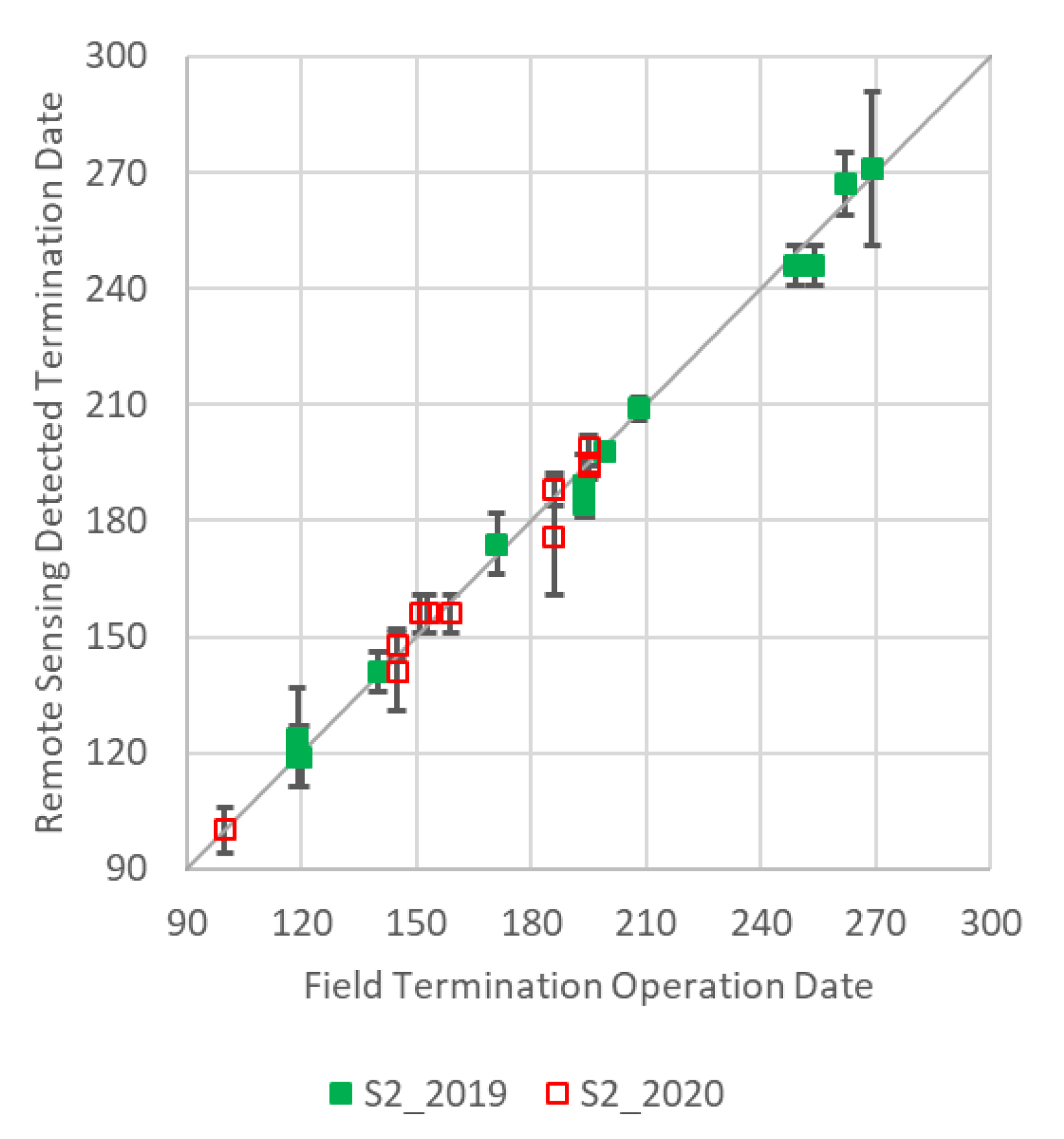
4.3. Field-Level Results from Sentinel-2

Using the same fields, we applied the WIST approach to the Sentinel-2 NDVI time-series. Figure 9 shows the termination dates from Sentinel-2 and the recorded harvest/termination dates. Comparing to results from VENµS in Figure 7, the Sentinel-2 time-series captured most of the terminations such as fields #4-25 (Figure 9c), #5-45 (Figure 9d), #5-2 (Figure 9f). However, fields #1-37 (Figure 9a) and #1-11 (Figure 9e) detected additional termination dates to those shown in Figure 7. For field #1-37 (Figure 9a), undetected clouds (not detected in the cloud mask algorithm) caused lower NDVI values and led to two downtrends and two false terminations. For field #1-11 (Figure 9e), a small peak in late June was caused by the regrowth of grasses before soybeans were planted on 28 June 2019. The decreasing momentum for the small peak was 0.022 from Sentinel-2. However, from the VENµS time-series, the momentum of MACD was smaller than 0.01, and the amplitude of NDVI was less than 0.15. This implies that the threshold of termination may be sensor dependent. Field #5-8 (Figure 9b) captured two terminated events but missed the first one on 20 May 2019, due to the lack of cloud-free observations, similar to field #5-9 in Figure 6. The closest observations around the first mowing date were 6 May 2019, and 15 June 2019 (lapse of 40 days). Grasses in the 15 June acquisition (25 days after mowing) have regrown. This example further demonstrates that frequent observations are critical for detecting cover crop termination.

Using the Sentinel-2 time-series, 27 harvest/terminations were correctly generated across 14 cover crop fields in 2019 and 2020. Two harvests (~7%) were missing due to the lack of observations. Three terminations (~10%) were falsely detected. Figure 10 shows the detected termination dates from Sentinel-2 compared to the recorded harvest operation dates. Even though Sentinel-2 revisit (5 day) was less frequent than VENµS (2 day), it still provided a good estimation of termination dates. Nevertheless, uncertainties (vertical bars) from Sentinel-2 are larger than VENµS. The largest uncertainty (20 days) was from field #5-8 due to the large gap (40 days) of cloud-free observations from 8 September 2019 (day 251) to 18 October 2019 (day 291), even though the termination estimate of 28 September 2019, was reasonable (harvest operation on 26 September 2019). Two terminations were not detected due to the lack of clear Sentinel-2 observations, and the downtrend was not significant, as in Figure 9b. Lowering the two thresholds for the MACD momentum and the NDVI amplitude can detect more termination dates; however, this may introduce more false detections. Ground information will be needed to determine appropriate thresholds. More discussion on the topic of thresholds is provided in Section 5.

4.4. Field Results from VENµS and Sentinel-2

Table 1. Statistics of termination dates from VENµS and Sentinel-2 over 29 harvest/termination events in 2019–2020.

	Mean Bias (Days)	Mean Abs. Difference (Days)	RMSE (Days)	Coefficient of Determination (R2)	Mean Uncertainty (Days)	Percent of Missing	Percent of False Detection
VENµS	0.4	2.1	2.6	0.998	3.5	0.0%	3.4%
Sentinel-2	−1.4	4.0	5.1	0.987	6.1	6.9%	10.3%

summarizes the statistics of terminations detected using the VENµS and Sentinel-2 time-series data. Both datasets produced reliable estimations of termination dates with a small bias (< 2 days) and a very high R² (>0.98). The mean uncertainties are within 4 days for VENµS and 7 days for Sentinel-2. The VENµS time-series captured all harvest operations for both years. There are about 7% of terminations missed from Sentinel-2. One out of 29 terminations (3.4%) from VENµS and three out of 29 terminations (10.3%) from Sentinel-2 were falsely detected. Results show that VENµS outperformed Sentinel-2 in all metrics due to higher temporal resolution.

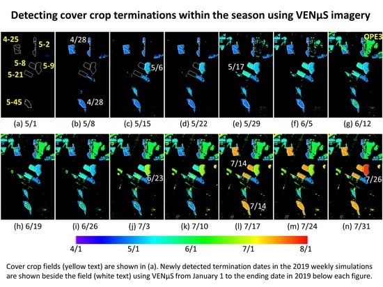
4.5. Near-Real-Time Mapping

Varying periods of VENµS NDVI time-series in 2019 were used to test near-real-time mapping capabilities of the WIST approach. In the simulation, we used all clear VENµS NDVI within the period until the ending date (the last day of available imagery). Data latency from satellite acquisition and processing was not included in the analysis. The simulations include weekly processing at the pixel level (image mode) and daily processing at the field level (text mode), using all available VENµS observations from 1 January 2019, to the ending date.

The pixel-level simulation used VENµS time-series images. Figure 11 shows the maps of weekly termination dates starting from 1 May 2019. We demonstrate results using the six fields in the east farm since they had multiple harvests and are close in space (subset area in Figure 3). In the simulated weekly processing, the VENµS time-series from 1 January to the ending day was used. The figure shows the latest termination dates before the ending date.

For the first run on 1 May 2019 (Figure 11a), no termination was detected in any field. On 8 May 2019 (Figure 11b), termination dates on 28 April 2019, for fields #4-25, #5-2, and #5-45 were detected. The FarmLogic database recorded the harvest date on 29 April 2019, for the three fields. On 15 May 2019 (Figure 11c), termination for field #5-9 was detected on 6 May 2019. The harvest operation was recorded on 7 May 2019. In the 29 May 2019 simulation (Figure 11e), termination dates were detected on 17 May 2019, for fields #5-8 and #5-21. Both fields were mowed on 20 May 2019, using a discbine machine. The estimated termination of 17 May 2019, was computed using the middle date of two observations on 10 May 2019, and 24 May 2019, as shown in Figure 12a. The lag time could be shortened if the process ran on an earlier date between 25 May and 28 May. In addition to six cover crop fields, the OPE3 (Optimizing Production inputs for Economic and Environmental Enhancement) field in the upper right of Figure 11g shows a termination date on 7 June 2019, a day before the planting date on 8 June 2019. The weeds in this field were killed by herbicide application before planting. It was regarded as a termination since the MACD momentum and NDVI amplitude were significant, as shown in Figure 12b. The simulated near-real-time process ending on 3 July 2019 (Figure 11j), detected a termination date of 23 June 2019, for field #5-9, which was close to the recorded harvest date on 20 June 2019. This was the second termination date in the record for that field, which was planted to alfalfa. The simulation of 17 July 2019 (Figure 11l) detected a new termination date of 14 July 2019, for four fields (#4-25, #5-8, #5-21, and #5-45). There were clear observations on 17 July 2019, and termination dates were detected just 3 days afterward. From the operation records, all four fields were mowed on 13 July 2019. However, field #5-21 shows mixed terminations. Figure 12c illustrates one pixel in field #5-21 (grass) whose termination was not detected, unlike in neighboring pixels, since the downtrend momentum and the amplitude of NDVI were smaller than the specified thresholds. In the last simulation (Figure 11n) ending on 31 July 2019, a termination date of 26 July 2019, was identified for field #5-9 (alfalfa). The recorded termination date was on 27 July 2019. It was the third detected termination date and the third recorded harvest date for this alfalfa field. In the simulation, all harvest events were detected correctly except for fields #5-21 and #5-45, which show some mixed termination dates from the two harvests. For field #5-21, some terminations were not detected, as illustrated in Figure 12c. For field #5-45, false detections were found for some pixels (Figure 11g–k) between two harvests (29 April 2019 and 13 July 2019). A small peak for field #5-45 was also shown in Figure 7d in early June but was not detected as a termination because the downward momentum and the amplitude of NDVI were not substantial at the field level. The lag time of detection ranges from 3–12 days in the weekly simulation process.

To investigate the capability of the WIST approach, we ran the near-real-time simulation daily for cover crop fields at field level (same dataset used as in Section 4.2 and Section 4.3) using VENµS data from both 2019 and 2020. Figure 13 shows the recorded harvest/mowing operation dates, the simulation ending dates of the first stable detection, and the detected termination dates using VENµS and Sentinel-2. All stable detections (same termination dates for at least a week) in the near-real-time simulations came from the first few detections, which means that early detected termination dates from the WIST algorithm are reliable. The thresholds for the MACD momentum (>0.01) and the NDVI amplitude (>0.15) are effective in our study area.

In Figure 13, both VENµS and Sentinel-2 captured the termination dates close to the recorded harvest/termination dates shortly after the machinery operation. VENµS time-series detected all termination events while the Sentinel-2 time-series missed three in the near-real-time simulation. The average biases of remote sensing estimations were 0.4 day from VENµS and 1.5 days from Sentinel-2. The average lag times of detection were about 4 days for VENµS and 8 days for Sentinel-2. Note that in the simulation, we have not considered the lag time of satellite data acquisition and processing. The total lag time of the near-real-time detection should be the sum of lag time from the WIST algorithm and the latency from satellite data acquisition and pre-processing.

5. Discussion

5.1. Performance and Comparison

Our results show that cover crop termination dates can be reliably detected using high temporal and spatial resolution satellite imagery. The proposed WIST algorithm uses the SG filter to generate daily NDVI and uses the MACD approach to detect a downward trend. Once the downtrend is confirmed by the momentum of MACD and the amplitude of NDVI, the termination date is determined using the original observations during the senescent period. The two dates with the most significant decreasing rate are selected to estimate the termination date and its uncertainty.

Many phenology algorithms have been developed in recent years. Most of them require multiple years of observations to generate annual phenology products. The annual phenology product for the target year could lag for several months to a year. The WIST algorithm can run in near-real-time whenever satellite data become available since both the SG filter and the MACD approach use a local moving-window technique. In our study, the average lag times of the WIST approach were about 4 days for VENµS and 8 days for Sentinel-2, not including the satellite data latency.

The global phenology products focus on major phenological metrics. The remote sensing phenological metrics are not the same as the crop physiological stage. Cover crop harvest/termination dates could be any day between the senescent onset and dormancy dates from remote sensing. The WIST algorithm can estimate cover crop termination dates directly. In addition, the WIST algorithm can detect all termination dates during the season or year, while most remote sensing phenology algorithms only detect a few seasonal cycles. For example, MODIS and VIIRS phenology products save two seasonal cycles in the annual phenology products [23]. For cover crops, as well as perennial hay crops such as alfalfa, the capability to map multiple terminations is desirable.

It is only recently that high temporal and spatial resolution satellite data, such as from Sentinel-2 and PlanetScope, have become available. Before the advent of Sentinel-2 and the HLS dataset, we used the data fusion approach using Landsat and MODIS/VIIRS [36] to generate high temporal and spatial resolution data to map crop phenology [25] and estimate crop yield [37]. Even for the daily satellite observations, clouds and cloud shadows affect the number of usable observations in the optical remote sensing. Cloud occurrence varies with location, date, and time. In BARC, the daily average cloud-free observations during the termination period were 14.8% for VENµS and 10.5% for Sentinel-2, which is typical for a temperate zone. The 2 days repeat VENµS observations (14.8% clear pixels) detected all termination events. The 4–5-day Sentinel-2 time-series (10.5% clear pixels) detected over 90% of termination events but had 10% false detections. Results may degrade over a cloudy region where the daily clear observations are less than 10%. The harmonized Landsat and Sentinel-2 (HLS) data product provides 3–4 days surface reflectance at 30 m spatial resolution. The global HLS data product will be routinely available starting in late 2020, with an expected data latency of about 5 days [38]. If we add 8 days of lag time from the WIST algorithm to confirm the downtrend based on the Sentinel-2 time-series, we may expect that cover crop termination dates to be detected within 2 weeks. In this study, we used the 10 m resolution VENµS (aggregated) and Sentinel-2 data, because our experimental fields are relatively large (>2 ha, 200 10 m pixels). The 5 m resolution VENµS data were not assessed but could be valuable for smaller fields. The 30 m resolution HLS data are detailed enough for application to most large commercial agricultural fields in the United States [39] where the farm field sizes typically are much larger than in our study area. HLS data have been used in mapping vegetation and crop phenology alone [24], or together with other coarse resolution data [40,41]. Data fusion based on HLS and MODIS/VIIRS may not be necessary for the cloud-clear regions to detect cover crop termination. Further study is needed for operational applications to standardize the processing (e.g., with/without data fusion) using HLS.

Machine learning approaches are suitable for detecting changes within a time-series. However, they require a large amount of ground data for training, which are hard to obtain. Unlike machine learning approaches, the WIST approach is built on the characteristics of cover crop termination and does not need large samples for training. The algorithm is simple and computationally efficient. In a Linux system (18 cores @ 3.07 GHz), the WIST algorithm took about 8 min to run all steps for the BARC site (1.5 million pixels). Most of the computing time was spent on the SG filter (first step). When ground truth is not available, the WIST algorithm can store the estimated termination dates, the uncertainty of estimations, the momentum of MACD, and the amplitude of NDVI for the retroactive decision or verification.

5.2. Constraints and Limitations

In the WIST algorithm, we used the momentum of MACD and the amplitude of NDVI to determine a significant downward trend. The thresholds were set to 0.01 for MACD and 0.15 for NDVI in this paper. These thresholds need to be assessed and potentially refined for other regions and cover crop types. A higher threshold requires a more significant downward trend and thus reduces false detection. This works better for green cover crops but may miss terminations for the sparse or less green cover crops when the change of NDVI after termination is not substantial. A lower threshold can detect more downward trends but may cause false detections. To determine appropriate thresholds for a cover crop in a region, an option is to save the momentum of MACD and the amplitude of NDVI for each pixel/field on each downtrend and then let users determine the thresholds using local ground data obtained afterward or a parameter optimization technique based on a history of recorded terminations for different cover types.

Cloudy or cloud-shadowed pixels leaked from imperfect cloud detection algorithms may affect the performance of the WIST algorithm. In this paper, noise has been reduced using two procedures. The first procedure implemented in the SG filter is to remove apparent spikes based on the fitting error (more than four standard deviations in this paper). The second procedure uses an average value in a moving window to determine the downward trend and the senescent period, avoiding the noise from a single day. However, several cases are a challenge for the WIST approach. First, multiple noise spikes (e.g., undetected clouds or cloud shadows) from successive days can cause false detection, such as the first two terminations shown in Figure 9a. The procedures introduced in this paper cannot handle multiple noise spikes in a row, a challenging case for any gap-filling and smoothing algorithm. Second, NDVI after termination may drop significantly, and it may be wrongly interpreted as a noise signal. In that case, the noise threshold in the SG filter needs to be relaxed more than in standard processing. Third, mis-registration in the time-series imagery can cause false detections near field boundaries. Estimation using field objects can reduce noise and geolocation errors by excluding pixels near the field boundaries, assuming the entire field was harvested on the same day. Finally, the WIST algorithm requires high-quality remote sensing data with a good cloud mask and geolocation accuracy.

Satellite observations in a time-series are not equally distributed due to clouds. The WIST algorithm estimates the termination date using two clear observations with the most significant decreasing rate during the senescent period. The actual termination date can be any date between the two observations. When the gaps between the two observations are large, the uncertainty of estimation will be more significant. Frequent satellite observations can produce a more accurate estimation with higher confidence (smaller uncertainty). In our study area, the 2 days repeat VENµS time-series produced accurate estimates with a mean uncertainty of 4 days compared to 6 days for the 4–5 days repeat Sentinel-2. The largest observed uncertainty of termination estimations was 8 days for VENµS and 20 days for Sentinel-2. Temporal frequency is crucial for the estimation of cover crop termination.

The WIST approach is more effective when the cover crops are terminated while still green. The approach is not valid for summer grain crops or winter grain crops such as wheat and barley, harvested at the end of the growing season when the plants dry down and leaves turn brown or yellow. In those cases, the change of NDVI before and after harvest may not be the most significant one during the senescent period. We found that the actual harvest operation dates for summer crops (corn and soybeans) and winter wheat occurred during the remotely sensed senescent period but closer to the dormancy (end of the season) dates rather than the detected termination dates. More studies are needed to accurately detect harvest dates for cash crops.

6. Conclusions

Mapping termination dates for cover crops within the season (or near-real-time) using remote sensing has been challenging in the past due to the lack of high temporal and spatial resolution data. In this paper, we used experimental VENµS (2 day) time-series data to develop a new within-season termination (WIST) algorithm for detecting cover crop termination dates. The WIST approach searches for downtrends of Vegetation Index time-series data and estimates termination date and uncertainty during a senescent period. The WIST algorithm employs a local moving window approach and can run in the near-real-time mode using any period of an imagery time-series. Results from the Beltsville Agricultural Research Center experimental fields in 2019 and 2020 show that termination dates can be reliably mapped using high temporal and spatial resolution time-series data. The VENµS time-series data with 2 days repeat produced accurate results with a mean absolute difference of 2 days. The Sentinel-2 (5 day) time-series also detected correct termination dates but gave 7% missing and 10% false detections. The average uncertainty of detected terminations was 4 days for VENµS and 6 days for Sentinel-2. A simulated mapping of termination in near-real-time shows that the average lag times of detection were about 4 days for VENµS and 8 days for Sentinel-2 after actual termination or harvest, not including latency of satellite data. This study demonstrates the potential to map cover crop termination within the season using high temporal and spatial resolution data for cover crop monitoring and agroecosystem services. Further work is needed for operational applications using routine satellite observations such as the Harmonized Landsat and Sentinel-2 (HLS) dataset.

References

1. Carlson, S.; Stockwell, R. Research priorities for advancing adoption of cover crops in agriculture-intensive regions. J. Agric. Food Syst. Commun. Dev. 2013, 3, 125–129. [Google Scholar] [CrossRef] [Green Version]
2. Dabney, S.A.; Delgado, J.A.; Reeves, D.W. Using winter cover crops to improve soil and water quality. Commun. Soil Sci. Plant. Anal. 2001, 32, 1221–1250. [Google Scholar] [CrossRef]
3. Reeves, D.W. Cover crops and rotations. In Crops Residue Management (Advances in Soil Science); Hatfield, J.L., Stewart, B.A., Eds.; Lewis Publishers: Boca Raton, FL, USA, 1994; pp. 125–172. [Google Scholar]
4. Sullivan, P. Overview of Cover Crops and Green Manures. National Center for Appropriate Technology. 2003. Available online: https://attra.ncat.org/product/Overview-of-Cover-Crops-and-Green-Manures/ (accessed on 21 September 2020).
5. De Baets, S.; Poesen, J.; Meermans, J.; Serlet, L. Cover crops and their erosion-reducing effects during concentrated flow erosion. Catena 2011, 85, 237–244. [Google Scholar] [CrossRef]
6. Hively, W.D.; Lang, M.; McCarty, G.W.; Keppler, J.; Sadeghi, A.; McConnell, L.L. Using satellite remote sensing to estimate winter cover crop nutrient uptake efficiency. J. Soil Water Conserv. 2009, 64, 303–313. [Google Scholar] [CrossRef] [Green Version]
7. Hively, W.D.; Lee, S.; Sadeghi, A.; McCarty, G.W.; Yeo, I.-Y.; Moglen, G. Estimating the effect of winter cover crops on nitrogen leaching using cost-share enrollment data, satellite remote sensing, and Soil and Water Assessment Tool (SWAT) modeling. J. Soil Water Conserv. 2020, 75, 362–375. [Google Scholar] [CrossRef]
8. Chesapeake Bay Program. Cover Crops Practices for use in Phase 6.0 of the Chesapeake Bay Program Watershed Model. Available online: https://www.chesapeakebay.net/documents/Phase_6_CC_EP_Final_Report_12-16-2016-NEW_TEMPLATE_FINAL.pdf (accessed on 21 September 2020).
9. Maryland Department of Agriculture. 2019/2020 Winter Cover Crop for Nutrient Management. Available online: https://mda.state.md.us/resource_conservation/counties/FY20_Program%20Requirements%20and%20Agreement_website.pdf (accessed on 21 September 2020).
10. Lawson, A.; Cogger, C.; Bary, A.; Fortuna, A. Influence of seeding ratio, planting date, and termination date on rye-hairy vetch cover crop mixture performance under organic management. PLoS ONE 2015, 10, e0129597. [Google Scholar] [CrossRef] [PubMed]
11. Hunt, E.R., Jr.; Hively, W.D.; McCarty, G.W.; Daughtry, C.S.T.; Forrestal, P.J.; Kratochvil, R.J.; Carr, J.L.; Allen, N.F.; Fox-Rabinovitz, J.R.; Miller, C.D. NIR-Green-Blue High-Resolution Digital Images for Assessment of Winter Cover Crop Biomass. GISci. Remote Sens. 2011, 48, 86–98. [Google Scholar] [CrossRef]
12. Prabhakara, K.; Hively, W.D.; McCarty, G.W. Evaluating the relationship between biomass, percent groundcover and remote sensing indices across six winter cover crop fields in Maryland, United States. Int. J. Appl. Earth Obs. Geoinf. 2015, 39, 88–102. [Google Scholar] [CrossRef] [Green Version]
13. Thieme, A.; Yadav, S.; Oddo, P.C.; Fitz, J.M.; McCartney, S.; King, L.; Keppler, J.; McCarty, G.W.; Hively, W.D. Using NASA Earth observations and Google Earth Engine to map winter cover crop conservation performance in the Chesapeake Bay watershed. Remote Sens. Environ. 2020, 248. [Google Scholar] [CrossRef]
14. European Space Agency (ESA). Sentinel-2 User Handbook. Available online: https://sentinels.copernicus.eu/documents/247904/685211/Sentinel-2_User_Handbook (accessed on 21 September 2020).
15. Claverie, M.; Ju, J.; Masek, J.G.; Dungan, J.L.; Vermote, E.F.; Roger, J.-C.; Skakun, S.V.; Justice, C. The Harmonized Landsat and Sentinel-2 surface reflectance data set. Remote Sens. Environ. 2018, 219, 145–161. [Google Scholar] [CrossRef]
16. Houborg, R.; McCabe, M.F. A Cubesat enabled Spatio-Temporal Enhancement Method (CESTEM) utilizing Planet, Landsat and MODIS data. Remote Sens. Environ. 2018, 209, 211–226. [Google Scholar] [CrossRef]
17. Dedieu, G.; Hagolle, O.; Karnieli, A.; Ferrier, P.; Crébassol, P.; Gamet, P.; Desjardins, C.; Yakov, M.; Cohen, M.; Hayun, E. VENµS: Performances and first results after 11 months in orbit. In Proceedings of the 2018 IEEE International Geoscience and Remote Sensing Symposium (IGARSS 2018), Valencia, Spain, 22–27 July 2018. [Google Scholar] [CrossRef]
18. Bar-Massada, A.; Sviri, A. Utilizing Vegetation and Environmental New Micro Spacecraft (VENµS) data to estimate live fuel moisture content in Israel’s mediterranean ecosystems. IEEE J. Sel. Top. Appl. Earth Obs. Remote Sens. 2020, 13, 3204–3212. [Google Scholar] [CrossRef]
19. Gao, F.; Anderson, M.C.; Daughtry, C.S.; Karnieli, A.; Hively, W.D.; Kustas, W.P. A within-season approach for detecting early growth stages in corn and soybean using high temporal and spatial resolution imagery. Remote Sens. Environ. 2020, 242, 111752. [Google Scholar] [CrossRef]
20. Jönsson, P.; Eklundh, L. TIMESAT—A program for analysing time-series of satellite sensor data. Comput. Geosci. 2004, 30, 833–845. [Google Scholar] [CrossRef] [Green Version]
21. Zhang, X.; Friedl, M.A.; Schaaf, C.B.; Strahler, A.H.; Hodges, J.C.F.; Gao, F.; Reed, B.C. Monitoring vegetation phenology using MODIS. Remote Sens. Environ. 2003, 84, 471–475. [Google Scholar] [CrossRef]
22. Gray, J.; Sulla-Menashe, D.; Friedl, M. User Guide to Collection 6 MODIS Land Cover Dynamics (MCD12Q2) Product. Available online: https://lpdaac.usgs.gov/documents/218/mcd12q2_v6_user_guide.pdf (accessed on 21 September 2020).
23. Zhang, X.; Liu, L.; Liu, Y.; Jayavelu, S.; Wang, J.; Moon, M.; Henebry, G.M.; Friedl, M.A.; Schaaf, C.B. Generation and evaluation of the VIIRS land surface phenology product. Remote Sens. Environ. 2018, 216, 212–229. [Google Scholar] [CrossRef]
24. Bolton, D.K.; Gray, J.M.; Melaas, E.K.; Moon, M.; Eklundh, L.; Friedl, M.A. Continental-scale land surface phenology from harmonized Landsat 8 and Sentinel-2 imagery. Remote Sens. Environ. 2020, 140, 111685. [Google Scholar] [CrossRef]
25. Gao, F.; Anderson, M.; Zhang, X.; Yang, Z.; Alfieri, J.; Kustas, B.; Mueller, R.; Johnson, D.; Prueger, J. Toward mapping crop progress at field scales through fusion of Landsat and MODIS imagery. Remote Sens. Environ. 2017, 188, 9–25. [Google Scholar] [CrossRef] [Green Version]
26. Roy, D.P.; Yan, L. Robust Landsat-based crop time series modelling. Remote Sens. Environ. 2020, 238, 110810. [Google Scholar] [CrossRef]
27. Yan, L.; Roy, D.P. Spatially and temporally complete Landsat reflectance time series modelling: The fill-and-fit approach. Remote Sens. Environ. 2020, 241. [Google Scholar] [CrossRef]
28. The Long-Term Agroecosystem Research (LTAR) Network. Available online: https://ltar.ars.usda.gov (accessed on 21 September 2020).
29. The Theia Data Center. Available online: https://theia.cnes.fr/atdistrib/rocket/#/search?collection=VENUS (accessed on 21 September 2020).
30. Hagolle, O.; Huc, M.; Desjardins, C.; Auer, S.; Richter, R. MAJA Algorithm Theoretical Basis Document (ATBD). Available online: https://www.theia-land.fr/wp-content-theia/uploads/sites/2/2018/12/atbd_maja_071217.pdf (accessed on 21 September 2020).
31. European Space Agency. The Copernicus Open Access Hub. Available online: https://scihub.copernicus.eu/dhus/#/home (accessed on 21 September 2020).
32. European Space Agency. The Sen2Cor tool. Available online: http://step.esa.int/main/third-party-plugins-2/sen2cor/sen2cor_v2-8/ (accessed on 21 September 2020).
33. Main-Knorn, M.; Pflug, B.; Louis, J.; Debaecker, V.; Müller-Wilm, U.; Gascon, F. Sen2Cor for Sentinel-2. In Proceedings of the SPIE Remote Sensing 2017, Warsaw, Poland, 11–24 September 2017; Volume 1042704. [Google Scholar] [CrossRef] [Green Version]
34. FarmLogic Systems. Available online: https://www.farmlogic.com/ (accessed on 21 September 2020).
35. Appel, G. Technical Analysis Power Tools for Active Investors; Financial Times Prentice Hall: Upper Saddle River, NJ, USA, 2005; p. 166. [Google Scholar]
36. Gao, F.; Masek, J.; Schwaller, M.; Hall, F. On the blending of the Landsat and MODIS surface reflectance: Predict daily Landsat surface reflectance. IEEE Trans. Geosci. Remote Sens. 2006, 44, 2207–2218. [Google Scholar]
37. Gao, F.; Anderson, M.; Daughtry, C.; Johnson, D. Assessing variability of corn and soybean yields in central Iowa using high spatiotemporal resolution multi-satellite imagery. Remote Sens. 2018, 10, 1489. [Google Scholar] [CrossRef] [Green Version]
38. The Harmonized Landsat-8 and Sentinel-2 (HLS) Data Product. Available online: https://hls.gsfc.nasa.gov/data/ (accessed on 21 September 2020).
39. Yan, L.; Roy, D.P. Conterminous United States crop field size quantification from multi-temporal Landsat data. Remote Sens. Environ. 2016, 172, 67–86. [Google Scholar] [CrossRef] [Green Version]
40. Liu, L.; Zhang, X.; Yu, Y.; Gao, F.; Yang, Z. Real-time monitoring of crop phenology in the midwestern United States using VIIRS observations. Remote Sens. 2018, 10, 1640. [Google Scholar] [CrossRef] [Green Version]
41. Zhang, X.; Wang, J.; Henebry, G.M.; Gao, F. Development and evaluation of a new algorithm for detecting 30 m land surface phenology from VIIRS and HLS time series. J. Photogr. Remote Sens. 2020, 161, 37–51. [Google Scholar] [CrossRef]
Figure 1. Beltsville Agricultural Research Center (BARC) study site (yellow rectangle and zoom-in figure, northeast suburbs of Washington D.C.). A VENµS false color composite image (Red: near-infrared band; Green: red band; Blue: green band) acquired on 13 July 2019, is overlaid on an Esri ArcGIS online base map.
Remotesensing 12 03524 g001
Figure 2. Percent of clear VENµS (a) and Sentinel-2 pixels (b) over BARC in 2019 and 2020. The cover crop termination periods are highlighted in light green.
Remotesensing 12 03524 g002
Figure 3. Cover crop fields (yellow polygons) in 2019 (yellow and white labels, 8 fields) and 2020 (green and white labels, 6 fields) over BARC were used in the validation. Four fields (white labels) planted cover crops in both years. Fields #1-37, #4-25, #5-8, and #5-9 (white labels) were planted with cover crops in both years. A total of 29 termination records for these fields in 2019 and 2020 were extracted. The text label near the field shows the field name used in BARC. The green rectangle is the sub-area for displaying near-real-time mapping detailed in Section 4.4. The basemap is a VENµS false color composite image (Red: near-infrared band; Green: red band; Blue: green band) acquired on 13 July 2019.
Remotesensing 12 03524 g003
Figure 4. An example diagram of NDVI and MACD shows the senescence onset (“s”), dormancy (“d”), and the termination date (“t”) of a winter cover crop (triticale and ryegrass mixture) detected from the NDVI and MACD time-series. The WIST algorithm detected a termination date of 28 April 2019 (red square) and the actual termination date was on 30 April 2019 (vertical red line). Dates t1 and t2 represent the period with the most rapid-rate of decrease of NDVI (defined in Section 3.1.3).
Remotesensing 12 03524 g004
Figure 5. Four terminations were detected for an alfalfa pixel (39.0210° N, 76.8467° W) in field #5-9 at the BARC using the VENµS NDVI time-series in 2019. All downward trends were significant, and the detected termination dates were close to the recorded harvest dates (vertical red lines).
Remotesensing 12 03524 g005
Figure 6. Three terminations were detected for the same alfalfa pixel as in Figure 5 (field #5-9) using the 2019. Sentinel-2 time-series. The first harvest on 7 May 2019, was missed since there were no clear Sentinel-2 observations from 7 May 2019 to 14 June 2019.
Remotesensing 12 03524 g006
Figure 7. Detected termination dates (red squares) from the VENµS time-series and the recorded harvest operation (vertical red lines) for six typical fields ((af), field name in the upper left) at the BARC with cover crops.
Remotesensing 12 03524 g007
Figure 8. Scatter plot of the detected termination dates for fields at the BARC in 2019–2020 using the VENµS NDVI time-series and the recorded harvest/termination operation dates. The vertical bar shows the uncertainty of the remote sensing estimated termination date.
Remotesensing 12 03524 g008
Figure 9. Detected termination dates (red squares) from the Sentinel-2 time-series and the recorded harvest operation (vertical red lines) for six typical cover crop fields ((af), field name in the upper left) in BARC.
Remotesensing 12 03524 g009
Figure 10. Scatter plot of the detected termination dates for fields at the BARC in 2019–2020 using the Sentinel-2 NDVI time-series and the recorded harvest operation dates. The vertical bar shows the uncertainty of the estimated termination date.
Remotesensing 12 03524 g010
Figure 11. Cover crop termination maps from the 14 weekly near-real-time simulations ((an), ending dates below subfigures) using VENµS images. Cover crop field names (yellow text) are shown in (a). Newly detected termination dates from six fields are shown beside the field (white text).
Remotesensing 12 03524 g011
Figure 12. Three examples from the near-real-time simulation from field #5-8 on 29 May (a), the OPE3 site on 12 June (b), and field #5-21 on 31 July (c), for explaining the weekly results in Figure 11e,g,n, respectively. Vertical red lines show the recorded harvest dates.
Remotesensing 12 03524 g012
Figure 13. The recorded harvest/termination operation dates, the detected termination dates, and the ending dates (the last day used in the simulation) from VENµS (_V) and Sentinel-2 (_S) in the daily near-real-time simulation for 29 harvests (x-axis) in 2019 and 2020. The x-axis shows the field name of each harvest. The dashed line separates harvests in 2019 and 2020.
Remotesensing 12 03524 g013