Abstract
Cotton root rot is a destructive cotton disease and significantly affects cotton quality and yield, and accurate identification of its distribution within fields is critical for cotton growers to control the disease effectively. In this study, Sentinel-2 images were used to explore the feasibility of creating classification maps and prescription maps for site-specific fungicide application. Eight cotton fields with different levels of root rot were selected and random forest (RF) was used to identify the optimal spectral indices and texture features of the Sentinel-2 images. Five optimal spectral indices (plant senescence reflectance index (PSRI), normalized difference vegetation index (NDVI), normalized difference water index (NDWI1), moisture stressed index (MSI), and renormalized difference vegetation index (RDVI)) and seven optimal texture features (Contrast 1, Dissimilarity 1, Entory 2, Mean 1, Variance 1, Homogeneity 1, and Second moment 2) were identified. Three binary logistic regression (BLR) models, including a spectral model, a texture model, and a spectral-texture model, were constructed for cotton root rot classification and prescription map creation. The results were compared with classification maps and prescription maps based on airborne imagery. Accuracy assessment showed that the accuracies of the classification maps for the spectral, texture, and spectral-texture models were 92.95%, 84.81%, and 91.87%, respectively, and the accuracies of the prescription maps for the three respective models were 90.83%, 87.14%, and 91.40%. These results confirmed that it was feasible to identify cotton root rot and create prescription maps using different features of Sentinel-2 imagery. The addition of texture features had little effect on the overall accuracy, but it could improve the ability to identify root rot areas. The producer’s accuracy (PA) for infested cotton in the classification maps for the texture model and the spectral-texture model was 2.82% and 1.07% higher, respectively, than that of the spectral model, and the PA for treatment zones in the prescription maps for the two respective models was 8.6% and 8.22% higher than that of the spectral model. Results based on the eight cotton fields showed that the spectral model was appropriate for the cotton fields with relatively severe infestation and the spectral-texture model was more appropriate for the cotton fields with low or moderate infestation.
1. Introduction
Cotton root rot, also known as Texas root rot, is caused by the soil-borne fungus Phymatotrichopsis omnivora. This disease occurs commonly in the southwestern and south central United States [1]. The leaves of the infested plant first turn yellow and then wilt rapidly, followed by plant death in a few days. Plant infection typically starts around the flowering stage and will continue for the rest of the season. Thus, the disease significantly reduces cotton yield and lowers lint quality [2]. Besides, the infested areas are stable across years, but the spatial distribution is not continuous across the field and the shapes of infested areas are irregular [3]. In early 2015, the Topguard Terra fungicide was registered to control the disease [4]. However, this fungicide is very expensive, so it is more cost-effective for farmers to apply the fungicide only to infested areas. Therefore, it is of great significance to map cotton root rot-infested areas for the management of this disease.
Remote sensing can monitor the dynamic changes of vegetation, and has been used as a useful tool for monitoring crop growth and identifying crop diseases, such as wheat yellow rust [5], bacterial leaf blight in rice [6], sclerotinia rot disease on celery [7], citrus greening disease [8]. When plants are infested with diseases, plant water content, pigment, and internal structure will change to varying degrees, resulting in changes in spectral reflectance [9]. Chen et al. [10] analyzed the canopy spectrum of Verticillium wilt of cotton and found that the visible light band of 680–760 nm and the near-infrared (NIR) band of 731–1371 nm had a significant response to the infection of Verticillium wilt. Shi et al. [11] quantitatively extracted and analyzed the hyperspectral wavelet characteristics of canopy of wheat stripe rust and powdery mildew. The results showed that the change of wavelet characteristics at 480, 633, and 943 nm could effectively diagnose and distinguish wheat stripe rust and powdery mildew stress. In addition, spectral features based on vegetation indices (VIs) can enhance and highlight some spectral changes, and are often used as features for crop disease monitoring. Zheng et al. [12] proposed the red edge disease stress index (REDSI) based on Sentinel-2 imagery, to detect yellow rust at the canopy and regional scales. De Castro et al. [13] showed the VIs using any of the bands related to red edge (740 and 750 nm) or NIR (760 and 850 nm), such as the transformed chlorophyll absorption in reflectance index (TCARI), the green normalized difference vegetation index (GNDVI), VIGreen and so on, had robustness in the ability of discriminating laurel wilt disease in avocado. The VIs including the green chlorophyll index (CIgreen), red-edge chlorophyll index (CIRE), normalized difference vegetation index (NDVI), and normalized difference red-edge index (NDRE) were proved to easily identify the banana Fusarium wilt disease [14]. However, spectral bands and VIs show different sensitivities to different crop diseases, so it is necessary to explore which spectral bands and VIs are suitable for the identification of specific diseases.
In practice, historical airborne and high-resolution satellite imagery were used to monitor cotton root rot and its changes [15,16], and NDVI proved to be an effective index for identifying root rot [17,18]. However, the availability of airborne imagery is affected by location and time of year and the cost is high. More recently, satellite imaging systems such as Sentinel-2 with fine spatial, spectral, and temporal resolutions have become freely available [19,20]. Additionally, the Sentinel-2 Multispectral Instrument (MSI) has three red-edge bands that are sensitive to the growth status of vegetation, which provide important information for monitoring the physiological status of plants [21,22]. For example, Lin et al. [23] suggested that the red-edge index from Sentinel-2 was suitable for spatiotemporal gross primary productivity (GPP) assessments. Chemura et al. [24] demonstrated that resampled Sentinel-2 sensor data had the potential for discriminating between coffee leaf rust (CLR) infestation severities (healthy, moderate, and severe). Fernández-Manso et al. [25] pointed out that Sentinel-2A red-edge spectral indices are adequate to discriminate burn severity. Song et al. [2] assessed the potential of the four Sentinel-2A bands (i.e., blue, green, red, and NIR) with 10 m spatial resolution for cotton root rot detection. Therefore, it is necessary to explore the potential of other spectral bands and VIs of Sentinel-2 in the identification of cotton root rot.
Image texture reflects the brightness nature of the image and its spatial arrangement of color, and different objects can be distinguished using different texture features [26]. Zhang et al. [27] used the gray-level co-occurrence matrix (GLCM) to extract texture features to identify grains. Texture features are similarly important indicators for crop growth monitoring [28,29]. When plants are infested by disease, the external characteristics changed significantly, such as morphology and texture. There have been studies using spatial features of images to monitor vegetation diseases. Wu et al. detected round-like crop lesion targets effectively using the improved Hough transform [30]. In addition, some studies show that combining texture features with spectral information have a certain impact on the results of remote sensing image classification [31]. Guo et al. [32] proved that the combination of spectral features and textural features significantly improved the identification accuracy of wheat yellow rust. The use of texture features and the combination of spectral and texture features to identify cotton root rot has not received much attention to date and requires further study.
In recent years, many methods and models have been used to select sensitive features to monitor and distinguish crop diseases [33]. The random forest (RF) algorithm, an integrated technology, could handle well large and high dimensional data [34], and is widely used in variable importance ranking. Zheng et al. [12] used the RF method to select three important bands in wheat yellow rust detection. Fletcher et al. [35] proved that the short-wave infrared band is the most important variable to distinguish soybean from two pigweeds using the RF algorithm. Binary logistic regression (BLR) is one of the most commonly used multivariate analysis methods, where the dependent variable is a binary variable that indicates whether an event exists [36]. BLR is a suitable method when the predictor variable has a binary nature, so it has certain potential in identifying crop diseases and insect pests. Ye et al. [14] showed that banana Fusarium wilt can be identified by VIs extracted from UAV-based multispectral imagery and the BLR method.
The overall goal of this study was to explore the potential of spectral indices and textural features of Sentinel-2 imagery and the combination of both for identifying root rot-infested cotton. The specific objectives were to (1) analyze the spectral difference between infested cotton and healthy cotton and identify optimal spectral indices by the RF algorithm; (2) extract the textural features using GLCM from the Sentinel-2 imagery and select optimal textural features using RF; (3) construct BLR models based on different features (spectral indices, textural features, and their combinations) and evaluate their performance for identifying cotton root rot and creating prescription maps.
2. Materials and Methods
2.1. Study Area
The study area was located in a cropping area with a history of serious cotton root rot near Edroy, Texas, USA (Figure 1). It covered a rectangular area of about 20.87 km2 (6.765 × 3.085 km), eight cotton fields with different levels of root rot were selected as shown in the figure. Field observations confirmed that cotton root rot was the dominant stressor and there was a minimal amount of interference from other biotic and abiotic factors in these cotton fields.
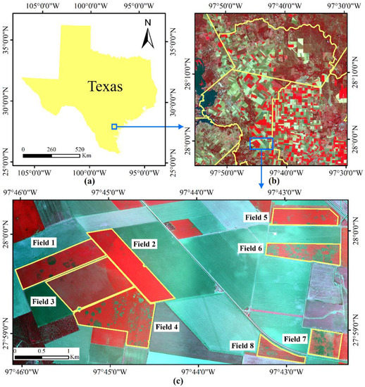
Figure 1.
Location of the study area and Sentinel-2 imagery. (a) Study site; (b) Sentinel-2A color infrared (CIR) composite image; (c) Airborne CIR composite image.
2.2. Image Acquisition and Processing
2.2.1. Airborne Multispectral Imagery
A two-camera airborne imaging system described by Song et al. [2] was used to acquire airborne imagery over the study area on 20 July 2016 under sunny conditions. The system consisted of two Nikon D810 digital CMOS cameras with Nikon AF Nikkor 20-mm f/1.8 G lenses (Nikon Inc., Melville, NY, USA). One camera captured red-green-blue (RGB) images, and the other camera was equipped with an 830-nm long-pass filter to obtain NIR images. Airborne images were acquired from a flying height of 3050 m above ground level with a ground speed of 225 km/h. The interval between the flight lines was spaced at 2500 m and the images were acquired at 5 s intervals to ensure at least 60% cross-track and along-track overlap. The images had a pixel array of 8353 × 3809 and a spatial resolution of 0.81 m. The Capture NX-D 1.2.1 software (Nikon Inc., Tokyo, Japan) was used to correct the images for vignetting and geometric distortion. Then the Pix4DMapper software (Pix4D Inc., Lausanne, Switzerland) was used for automatic image mosaicking. The images were mosaicked using ground control points (GCPs) in Pix4DMapper software to improve the positional accuracy. The mosaicked RGB and NIR images were combined as a four-band mosaicked image. The Quick Atmospheric Correction tool in ENVI 5.3 (Harris Corporation, Jersey City, NJ, USA) was used for image atmospheric correction [2]. According to Yang et al. [6], two unsupervised classification methods and six supervised classification methods were accurate for identifying cotton root rot. Among them, the neural net technique uses standard back propagation for supervised learning [37]. Learning occurred by adjusting the weights in the node to minimize the difference between the output node activation and the output. In this study, neural network classification methods (ENVI 5.3, 2016) were applied to airborne multispectral images to identify the root rot-infested area of each cotton field, the total numbers of training pixels for the eight fields were 19,724 (0.29% of the total area) for the infested class and 30,160 (0.44% of the total area) for the noninfested class. In all the classifications, the process finished when the number of iterations reached 1000 or the training RMS reached 0.01. The classification results of each field was compared with the original imagery and field observations and the result was used as the reference of cotton root rot classification in the study area.
In addition, the 0.81 m airborne image was resized to 10 m spatial resolution with bilinear method. The airborne image was used as the reference image for Sentinel-2A image geometric correction [2].
2.2.2. Sentinel-2 Satellite Imagery
Sentinel-2 is a wide-range, high-resolution, multispectral imaging mission created by the European Space Agency (ESA). It consists of two polar-orbiting satellites placed in the same orbit, Sentinel-2A and Sentinel-2B. Sentinel-2 is free to use and the revisit cycle is 10 days (or 5 days when two satellites are operating simultaneously). Sentinel-2 images cover 13 bands in the visible, NIR, and shortwave infrared (SWIR) wavelengths with three different spatial resolutions [24].
In this study, the Sentinel-2 multispectral image acquired on 11 July 2016 was downloaded from https://scihub.copernicus.eu/. Atmospheric correction of the image was performed using the Sen2cor toolbox (provided by ESA). Four bands (R, G, B, and NIR) with 10 m spatial resolution and six bands (3 red-edge, Narrow NIR, 2 SWIR) with 20 m spatial resolution were selected as the data source. For the purpose of image analysis, the bands with 20 m spatial resolution were resampled to a pixel size of 10 m. Then we used the resized 10 m airborne image to correct the Sentinel-2A dataset with registration module in ENVI 5.3. The Sentinel-2A CIR composite image for the study area is shown in Figure 2.
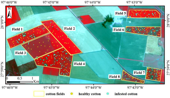
Figure 2.
Sentinel-2A color infrared (CIR) composite image with ground verification points for the study area.
2.3. Methods
Figure 3 presents the research workflow of cotton root rot identification based on multifeature selection from Sentinel-2 image. It mainly includes four steps: (1) the airborne multispectral imagery was processed, and the cotton root rot classification and prescription maps based on the processed imagery were generated. (2) Spectral characteristics of the infested and healthy cotton in Sentinel-2A were analyzed; the spectral indices and texture features were extracted; the optimal spectral indices and texture features were identified by the RF. (3) Three BLR models were established using different features based on spectral indices, texture features, and a mixture of spectral indices and texture features, respectively, and the corresponding cotton root rot classification and prescription maps were generated. (4) Confusion matrices, the overall accuracy (OA), producer’s accuracy (PA), and user’s accuracy (UA) were used to evaluate the feasibility of generating classification and prescription maps based on Sentinel-2 imagery.
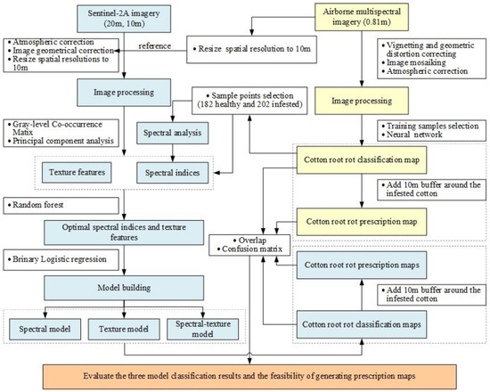
Figure 3.
Flowchart of data analysis and processing.
2.3.1. Spectral Characteristics Analysis
In order to analyze the spectral difference between infested cotton and healthy cotton in Sentinel-2A, 384 points (182 healthy and 202 infested) were selected from the eight fields based on the classification results of the airborne multispectral images. Additionally, the 384 points selected were ground checked by the field crew to confirm the infestation status, the number of these points in each field is shown in Table 1.

Table 1.
The number of sample points in healthy and infested cotton areas for Fields 1–8.
These points were overlaid on the preprocessed Sentinel-2A imagery and the reflectance values were extracted. The spatial distribution of these points is shown in Figure 2. The spectral reflectance values of the 384 points are shown with box-scatterplots in Figure 4. As can be seen from the figure, the reflectance of infested cotton in the bands of 497–704 nm was higher than that of healthy cotton. The average reflectance in the bands of 740–865 nm of healthy cotton was remarkably higher than that of infested cotton with a difference of about 0.09–0.15. In the bands of 1614 and 2202 nm, which are sensitive to the response of crop moisture, the reflectance of infested cotton was higher than that of healthy cotton.
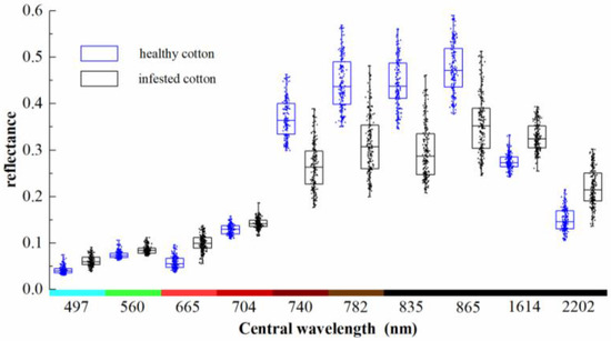
Figure 4.
Box-scatterplots of reflectance of healthy cotton and root rot-infested cotton.
2.3.2. Extraction of Spectral Indices
Spectral indices are combinations of spectral reflectance from two or more wavelengths, which can enhance the spectral difference between infested and healthy cotton. The biophysical and biochemical crop variables, such as canopy structure, leaf pigment, and canopy water content are changed when cotton is infested with root rot. In this study, 10 spectral indices (Table 2) related to different physiological parameters were selected from the literature on crop diseases and they were further tested for their ability to detect cotton root rot infestation in this study.
Table 2.
Spectral indices used for the identification of cotton root rot in this study.
2.3.3. Extraction of Texture Features
The multispectral bands or spectral indices of satellite imagery are often used to identify infested plants with a classification technique [47]. Most of these techniques, however, only look at the spectral values of individual pixels and do not take the spatial context of pixels into consideration. Texture can be defined as the various measures of smoothness, coarseness, and regularity of an image region [26]. When crops are infested by disease, changes in pigment, water content of the plants result in spectral changes, as well as changes in the canopy structure and the morphology, causing textural changes. Previous studies have shown that it is feasible to identify the crop diseases based on texture features [32]. The popular GLCM texture model [48] has been widely used to extract texture features of images, for this study, the following eight widely used GLCM texture features were selected: contrast, dissimilarity, homogeneity, angular second moment, entropy, mean, variance, and correlation.
In order to reduce the data redundancy of multispectral bands without significantly reducing the information content in the image, principal component analysis (PCA) [49] was performed on the Sentinel-2A multispectral data in ENVI 5.3 and the first two principal component (PC) images (with more than 98% of the cumulative variance) were chosen. The 16 texture features of the first two PC images were extracted by GLCM. Considering the accuracy and efficiency, the processing window was set to 3 × 3, the co-occurrence shift X and Y were set to 1 and 1, and the greyscale quantization levels was set to 64. Then, the 16 texture features were abbreviated as the texture features and numbers. For example, the mean of the first PC images is abbreviated as “Mean 1”, the variance of the second PC images is abbreviated as “Variance 1”.
2.3.4. Selection of Optimal Spectral Indices and Texture Features
RF is an ensemble of learning algorithms proposed by Breiman [35]. During the forest construction process, the randomness is not only in the selection of the data set, but also in the selection of the feature set. Using Bootstrap sampling technology to extract N samples from the original sample as a training set, and rather than choosing the best split among all attributes, m attributes are randomly chosen from M at each node and then these m attributes are used to split the node according to the principle of the decision tree algorithm, where m << M, to find the best segmentation feature. This study uses the Gini index to measure the effect of feature segmentation when performing node segmentation. Suppose there are classes in the sample , then its Gini index is
where, is the probability of occurrence of the first sample. If after a split, the sample set is divided into parts , then the Gini index for this split is
The value of the Gini index is related to the segmentation effect. The larger the value, the more important the feature is. This study uses the RF algorithm to select the sensitive spectral indices and texture features for identifying cotton root rot.
The values of 10 spectral indices and 16 texture features of the 384 sample points were extracted using ArcGIS 10.2 as the sample set. In order to avoid the instability of the experimental results, the cross-validation method was used in feature selection, and the sample set was divided into a training set and a test set according to a 3:1 ratio, and the proportion of the class before segmentation was maintained.
2.3.5. Binary Logistic Regression
In this study, spectral and texture features were used to establish BLR models. Mark infested cotton as 1 and healthy cotton as 0. Limit the range of the dependent variable to [0, 1]. Set the conditional probability of cotton root rot to be P and is assumed to be a functional form of a variable. Logit transformation is performed to build a BLR model [14,36].
BLR model takes the form of
can be expressed as
In the formula, are regression coefficients; are regression independent variables.
In this study, the regression independent variables were the spectral indices and texture features selected by the RF algorithm and their combinations, and the sample set was divided into the training set and the test set according to a 3:1 ratio by random sampling. A stepwise method was used to establish three BLR models: spectral, texture, and spectral-texture. In the process, the variables entered the equation based on the significance of the score statistics and were removed from the equation based on the probability of the likelihood ratio statistics based on the conditional parameter estimation.
In order to evaluate the classification accuracy of the BLR models using the sample set, the Precision, Accuracy, Recall, and F-score were selected as the evaluation indicators.
where TP is true positive; FP is false positive; TN is true negative; FN is false negative.
2.3.6. Buffer Creation and Accuracy Assessment
The 0.81 m airborne image subset by field was used to detect the cotton root rot-infested areas for each field. The results for all cotton fields were combined to a cotton root rot reference classification map. To accommodate the temporal variation and potential expansion of the disease from year to year, a 3–10 m buffer was usually added around the infested areas to become part of the treatment areas when prescription maps were created from fine-resolution airborne imagery [4]. In this study, a 10 m buffer (same as the pixel size of Sentinel-2 imagery) was added around the infested areas based on the airborne classification result to generate the reference prescription map for the study area.
The BLR models constructed by the optimal spectral indices, texture features, and their combinations were applied to the Sentinel-2 images on the pixel level to detect the cotton root rot-infested areas for the eight fields and generate the classification maps. Similarly, a 10 m buffer was added around the infested areas to generate the prescription maps.
In order to evaluate the feasibility of different Sentinel-2A features for identifying cotton root rot and creating prescription maps, the classification maps and prescription maps of three BLR models were exported to ArcGIS 10.2, which were then intersected with the classification map and prescription map of the airborne images, respectively. For quantitative accuracy assessment of the classification results, error matrices were used to determine the performance, OA, PA, and UA [50,51].
3. Results
3.1. Selection of Optimal Spectral Indices and Texture Features for Identifying Cotton Root Rot
The RF algorithm was used to select the sensitive spectral indices and texture features for identifying cotton root rot. The results are shown in Figure 5. From Figure 5a, PSRI had the most significant impact on cotton root rot classification, followed by NDVI, NDWI1, MSI, and RDVI. Among them, PSRI, which indicates the state of canopy senescence, was the most important spectral index for cotton root rot identification. NDWI1 and MSI provide a measure of the amount of water contained in the canopy foliage. NDVI and RDVI are related to the general quantity and vigor of green vegetation. The first five spectral indices were selected to build the BLR model.
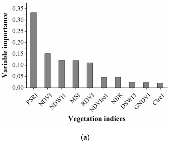
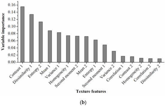
Figure 5.
Rankings of (a) spectral indices and (b) texture features based on their importance for cotton root rot classification through random forest (RF) models.
From Figure 5b, it was obvious that Contrast 1 was the most important texture feature for cotton root rot classification, followed by Dissimilarity 1, Entory 2, Mean 1, Variance 1, Homogeneity 1, and Second moment 2. The remaining features had little impact on cotton root rot identification, therefore, the first seven important texture features were selected to build the BLR model.
3.2. Binary Logistic Regression Models with Different Features
Table 3 presents the variables and parameters of BLR models. All the variables in the three models had a significant level of less than 0.05. The BLR models are shown as formulas 10–12.
Table 3.
Selected features and regression parameters.
The classification accuracies of the BLR models with the sample set are shown in Table 4. For the whole data set, Precision, Accuracy, Recall, and F-score were approximately equal in value and had the same trend among the three models, indicating that the classification sample distribution was balanced, and the accuracy rate could be used to evaluate the classification accuracy of each model. The Precision, Accuracy, Recall, and F-score of the three models exceeded 95% for the training set. The Precision was higher for the test set, while the Accuracy, Recall, and F-score were lower. Additionally, the Recall was less than 0.9 in the spectral and textural models for the test set. The classification accuracy of the spectral-texture model was slightly higher than that of the texture model or the spectral model.
Table 4.
Classification accuracy of binary logistic regression (BLR) models.
3.3. Classification Results and Accuracy Assessment
3.3.1. Airborne and Sentinel-2A Image Classification Results
Table 5 lists the field area and the cotton root rot-infested areas from classification maps generated from the airborne images and Sentinel-2A images for Fields 1–8. The cotton root rot classification results generated from the airborne images showed that the total infested area for the eight fields was 560,286 m2 with an average infestation percentage of 12.86% for the whole study area. The percentage of root rot-infested areas for Fields 1–8 ranged from 0.35% for Field 3 to 48.16% for Field 7. Among them, Fields 1–3 and 5 had relatively low level of infestation (low infestation), while Fields 4 and 8 had medium level of infestation (moderate infestation), and Fields 6 and 7 had high level of infestation (severe infestation). The cotton root rot classification results generated from the Sentinel-2A images showed more root rot-infested areas. The classification result of the spectral model showed that the total infested area estimated was 752,623 m2 and the average infestation percentage was 17.27%, and the percentage of root rot-infested areas for Fields 1–8 ranged from 0.26% to 61.66%. For the texture model, the total infested area was estimated to be 1,139,019 m2 with an average infestation percentage of 26.13%, and the percentage of root rot-infested areas for Fields 1–8 ranged from 1.54% to 75.05%. For the spectral-texture model, the total infested area was 811428m2 and the average infestation percentage was 18.62% with the infestation percentage among the eight fields ranging from 1.22% to 57.50%. Clearly, the classification results of the spectral model were most similar to those of the airborne images, followed by the spectral-texture model and the area of root rot identified by the texture model was the largest.
Table 5.
Cotton root rot-infested areas of classification maps generated from airborne images and Sentinel-2A images for Fields 1–8.
3.3.2. Sentinel-2A Image Classification Accuracy Assessment
The classification results of Sentinel-2A images based on the spectral model, texture model, and spectral-texture model were overlaid with the airborne image classification results, respectively, and the results are shown in Figure 6. The green zone in Figure 6 shows the cotton root rot-infested areas detected by both the airborne and Sentinel-2A images, indicating the correctly classified areas in the Sentinel-2A image. The blue zone depicts the cotton root rot-infested areas detected by the Sentinel-2A image but not detected by the airborne image, which indicates the commission area for the Sentinel-2A image. The orange zone in Figure 6 is the cotton root rot-infested areas only detected by the airborne image, which indicate the areas omitted by the Sentinel-2A image.
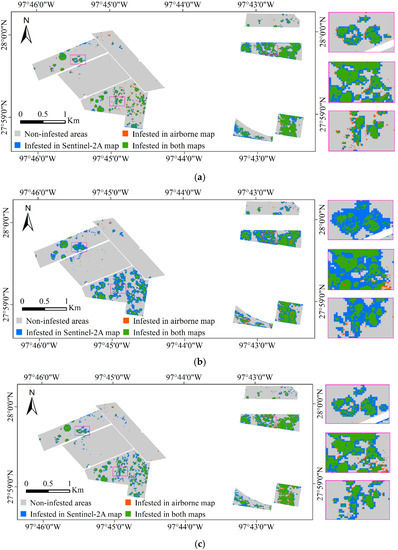
Figure 6.
Overlaid cotton root rot classification maps from airborne and Sentinel-2A images for Fields 1–8 and the zoomed in rectangle scenes for the areas marked on the maps are shown at the right. (a) Sentinel-2A classification map based on the spectral model; (b) Sentinel-2A classification map based on the texture model; (c) Sentinel-2A classification map based on the spectral-texture model.
From Table 6 and Figure 6, the classification accuracy of the spectral model, texture model, and spectral-texture model was 92.95%, 84.81%, 91.87%, respectively. The spectral model produced the highest OA to identify root rot-infested cotton, followed by the spectral-texture model and the texture model. In the classification results of the spectral model, the PA, which indicates the probability of actual areas being correctly classified, was 89.73% for the root rot category and 93.42% for the noninfested category. In other words, 89.73% (the green zones in Figure 6a) of the root rot areas were correctly identified as root rot, while 93.42% of the noninfested areas (the gray zones in Figure 6a) were correctly identified as noninfested in the classification map. Additionally, with spectral model, 10.27% of the root rot-infested areas were omitted by the Sentinel-2A image. The PA of the texture model and the spectral-texture model were 92.55% and 90.80%, respectively, for the infested category, which means that more root rot areas were identified with the texture model and the spectral-texture model. At the same time, the UA for the infested category of the texture model and the spectral-texture model was lower than that of the spectral model, indicating that more commission areas (the blue zones in Figure 6b,c) were generated from the Sentinel-2A image with the texture model and the spectral-texture model. The PA and UA for the infested category of the spectral-texture model were 90.80% and 62.70%, respectively.
Table 6.
Error matrices for classification maps generated by binary logistic regression (BLR) models for the whole study area.
Figure 7 illustrates the differences in the OA, PA, and UA for the infested category for Fields 1–8 based on the spectral model, texture model and spectral-texture model. From Figure 7a, the spectral model achieved the best OA in the discrimination between healthy and infested cotton for Fields 1–5, which had relatively low infestation, followed by the spectral-texture model and the texture model. The spectral-texture model achieved the best OA for Fields 6–8, which had relatively high infestation, followed by the spectral model and the texture model. The overall accuracies of the texture model and spectral-texture model for Fields 1–7 were higher than 80%. From Figure 7b, the PA for the infested category based on the three models was higher than 80% for Fields 1 and 4–7. In addition, combining the spectral and texture features could enhance the performance of detecting more root rot areas, thus resulting in higher PA in cotton fields with low and medium levels of infestation. The UA for the infested category based on the three models was almost below 80% for all fields (Figure 7c), indicating that higher than 20% of the infested areas on the classification map were actually healthy areas for all fields. Moreover, the commission error of the texture model was the highest for all fields. The UA for the infested category of Fields 6 and 7 with severe infestation was higher than that for the other fields. This result indicates that it is feasible to identify cotton root rot in fields with moderate and severe infestation using different features, especially spectral features, and combinations of spectral and texture features. However, it has certain limitations in identifying cotton root rot with Sentinel-2A images for fields with less than 1% infestation.
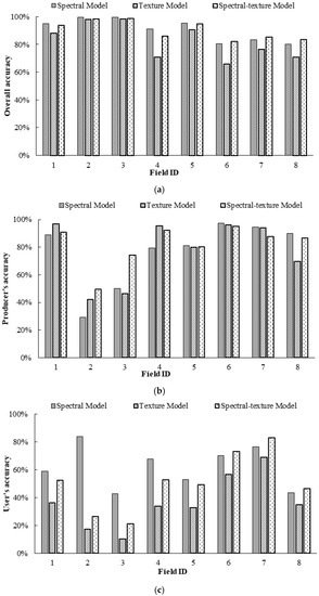
Figure 7.
Comparison of classification accuracy of classification maps generated by binary logistic regression (BLR) models: (a) overall accuracy (OA); (b) producer’s accuracy (PA) for the infested category; (c) user’s accuracy (UA) for the infested category.
3.4. Feasibility for Creating Prescription Maps
A 10 m buffer was added to the infested areas of the airborne and Sentinel-2A classification maps in this study to generate prescription maps. Table 7 lists the treatment areas of the prescription maps generated from the airborne and Sentinel-2A images for Fields 1–8. For the airborne prescription map, the total treatment area reached 31.2% with a 10 m buffer. The average treatment percentages for the spectral model, texture model and spectral-texture model were 27.58%, 36.64%, and 32.14%, respectively, for all the fields, and these percentages were similar to the percentage (31.20%) from the airborne image. Clearly, the treatment area for each field was significantly increased with the addition of the buffer zones. The reason for the large increase was that the small polygons representing root rot-infested areas on the classification maps expanded in all directions and filled the gaps between the polygons with addition of the buffer.
Table 7.
Treatment areas of prescription maps generated from airborne and Sentinel-2A images for Fields 1–8.
Figure 8 shows the results of overlaying the prescription maps from the airborne and Sentinel-2A images for Fields 1–8, and Table 8 shows the accuracy assessment error matrix for the prescription maps from the Sentinel-2A images for all the eight fields. The spectral-texture model achieved the best OA (91.40%), followed by the spectral model and the texture model with an OA of 90.83% and 87.14%, respectively. The PA of the spectral model, texture model, and spectral-texture model was 95.97%, 86.70%, and 93.06%, respectively, for the nontreatment category and 79.50%, 88.10%, and 87.72%, respectively, for the treatment category. The treatment areas that were not generated by the Sentinel-2A image were mainly composed of some small root rot-infested areas (< 10 m) and their buffered areas on the airborne prescription map (the orange zones in Figure 8). The UA of the texture model for the treatment category was 75.05%, indicating that 24.95% of the infested areas on the prescription map were actually nontreatment areas. The UA of the spectral model and the spectral-texture model was 89.94% and 85.15%, respectively. Therefore, the commission error of the texture model was the highest, followed by the spectral-texture model and the spectral model. Above all, it was feasible to create the prescription maps with the Sentinel-2A images. Moreover, the spectral-texture model had the highest accuracy. In practical applications, the selection of the optimal buffer distance depends on factors such as infestation pattern, planting swath, and the producer’s risk tolerance. A buffer size of 10 m is practical, especially if Sentinel-2 imagery is used. If the farmer wants to make sure all potential root areas are treated or if the application equipment has a wider swath, a larger buffer can be used. At any rate, site-specific fungicide treatment significantly reduces the fungicide use and increases the farming profit.
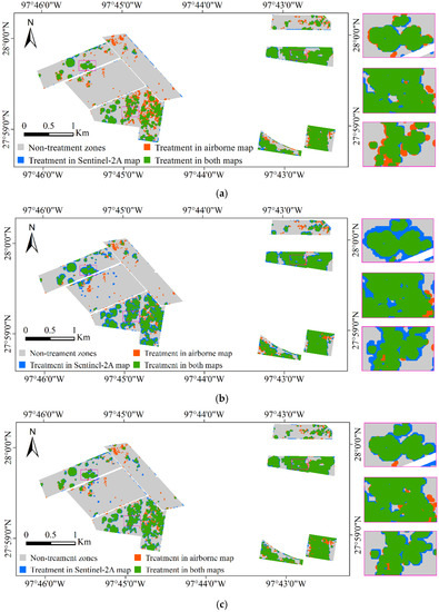
Figure 8.
Overlaid prescription maps from airborne and Sentinel-2A images for Fields 1–8 and the zoomed in rectangle scenes for the areas marked on the maps are shown at the right. (a) Sentinel-2A prescription map based on the spectral model; (b) Sentinel-2A prescription map based on the texture model; (c) Sentinel-2A prescription map based on the spectral-texture model.
Table 8.
Error matrices for prescription maps generated by binary logistic regression (BLR) models for the whole study area.
Figure 9 illustrates the OA, PA, and UA for the treatment category of the prescription maps generated from the Sentinel-2A images by the three BLR models for Fields 1–8. From Figure 9a, the spectral model achieved the best OA for Fields 1, 3, 5, and 7, followed by the spectral-texture model and the texture model, while the spectral-texture model achieved the best OA for Fields 2, 4, 5, and 8, followed by the spectral model and the texture model. From Figure 9b, the PA for the treatment category based on the spectral-texture model was the highest for Fields 1–5, while the PA for the treatment category based on the spectral model was the highest for Fields 6–8. From Figure 9c, the UA for the treatment category based on the spectral model was the highest for Fields 1, 3–5, and 7, while the UA for the treatment category based on the spectral-texture model was the highest for Fields 2, 6, and 8. This result indicates that it is feasible to create prescription maps using different features of Sentinel-2A images. The spectral-texture model has certain advantages for cotton fields with low or moderate infestation, while the spectral model is more suitable for severely infested cotton fields.
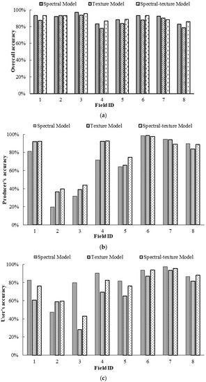
Figure 9.
Comparison of classification accuracy of prescription maps generated from Sentinel images by three binary logistic regression (BLR) models for Fields 1–8: (a) overall accuracy (OA); (b) producer’s accuracy (PA) for the treatment category; (c) user’s accuracy (UA) for the treatment category.
4. Discussion
Remote sensing technology has long been used for detecting and mapping crop diseases [52,53]. The Sentinel-2 MSI sensor with refined spatial, spectral, and temporal resolutions is considered to have great potential in estimating and monitoring the biophysical state of plants for precision agriculture [54,55,56].
The biophysical and biochemical crop features, such as canopy structure, leaf pigment, and water content change when plants are stressed by diseases [57]. These changes will alter crop canopy reflectance that can be remotely sensed. Based on the results of this study, infested cotton had higher spectral reflectance in 497–704 nm, exhibited a downward reflectance trend in 740–865 nm, and had higher reflectance at 1614 and 2202 nm, compared with healthy cotton. This is attributed to the fact that the leaves of root rot-infested plants turn yellow and brown and then wilt rapidly, causing the reduction of chlorophyll content and the loss of plant water content. There were significant differences in spectral reflectance between infested cotton and healthy cotton due to these changes. Generally, compared with the reflectance of healthy plants, the chlorophyll of diseased plants is significantly reduced, and the ability to absorb visible light is reduced, resulting in higher reflectance in the visible regions. The plant structure is seriously damaged, which reduces the spectral reflectance in the NIR region. Therefore, the spectral reflectance of diseased plants is higher in the visible regions and lower in the NIR region [58]. The research by Kakani et al. also demonstrated that the cotton leaf water content had a significant negative correlation with the reflectance in 460–514, 605–698, 1412–1818, and 1933–2479 nm wavebands, and a significant positive correlation with the reflectance in the 727–1345 nm band [59].
The spectral indices can highlight the difference between diseased and healthy plants, and at the same time reduce the influence of factors such as soil and atmosphere [32]. In this study, 10 spectral indices related to canopy structure, pigment content, water content, and leaf senescence [5,12,13,24,42,60,61] were extracted. Then, the RF algorithm was used and five optimal spectral indices sensitive to cotton root rot were selected to establish models. The OA of the infested category in the classification map for the spectral model was 92.95%, and the PA was 89.73%, indicating that the spectral indices alone are useful for identifying cotton root rot. Yang et al. [17] demonstrated that NDVI derived from airborne images achieved good results for identifying cotton root rot. Then, we used the spectral model to generate prescription maps, the OA and PA reached 90.83% and 79.50%, respectively. The reason for the decrease in PA was that some small root rot-infested areas were not identified by the spectral model, and the area increased with the buffer was added to these areas. RF, which could handle well large and high dimensional data, has the ability to produce a variable importance ranking. This information is valuable for the user to select variables to build simpler, more readily interpretable models [62]. Zheng et al. [12] also used the RF method to obtain the optimal bands for the Sentinel-2 sensor and achieved satisfactory result in wheat yellow rust detection.
In this study, 16 texture features were extracted from Sentinel-2A images, and seven sensitive texture features were selected using RF to build model for identifying root rot. The OA and PA of the infested category in the classification map for the texture model were 84.81% and 92.55%, respectively. Clearly, the PA for the infested category was higher than that of the spectral model, because more cotton root rot areas could be identified using the texture information. This is attributed to the fact that diseased cotton not only has obvious changes in spectral characteristics, but also differs from healthy cotton in texture characteristics. In July, healthy cotton had a large leaf area and dense canopy, and cotton root rot was also fully pronounced. Dark stalks and dead leaves attached to infested cotton plants greatly changed the canopy morphology and structure of the plants, causing changes in texture features. Guo et al. used image texture to detect diseases of wheat yellow rust and obtained an encouraging result [32]. When using this model to generate prescription maps, OA and PA for the treatment category were 87.14% and 88.10%, respectively. The PA was 8.60% higher than that of the spectral model. This is also due to the ability of texture features for more root rot recognition. However, texture represents the spatial properties of an image region [26], edge effects could cause some healthy cotton around the infested areas to be misclassified as infested cotton. As a result, classification commission errors for cotton root rot-infested areas were increased with the texture model.
When the spectral-texture model was used to identify cotton root rot, the OA and PA for the infested category in the classification map were 91.87% and 90.80%, respectively. The OA was 1.08% lower than that of the spectral model and the PA was 1.07% higher than that of the spectral model, while OA was 7.06% higher than that of the texture model and the PA was 1.75% lower than of the texture model. The reason for this mixed result may be that the combination of spectral and texture features could increase the ability to identify root rot areas, and at the same time, it could weaken, to a certain extent, the edge effect generated by texture features alone. However, it can be seen from Figure 6 that the blue areas were still more than those of the spectral model, causing the UA and OA to be 4.10% and 1.08%, respectively, lower than those of the spectral model. The OA and PA of the prescription map were 91.40% and 87.72%, respectively, using the spectral-texture model. They were 0.57% and 8.22% higher than the respective values of the spectral model, and the OA was 4.26% higher and the PA was 0.38% lower than the respective values of the texture model. Overall, it can be seen that the addition of texture features had little effect on the OA, but it could improve the ability to identify root rot areas. In a study of a crop classification decision model, Peña-Barragán et al. [63] revealed that the contribution of texture features was not decisive compared with multispectral features such as NDVI. In addition, as other studies have reported [64] that how texture information provides positive or negative effects on the classification is complex, and how the texture characteristics are affected by object heterogeneity or image spatial resolution need future studies. Thus, the reason that the texture feature did not have a positive effect for the OA as additional information in our study is likely due to the Senitnel-2A spatial resolution.
Cotton planting time varies from late March to early April every year in the study area (Edroy, Texas), and the cotton growth and field management practices for different fields differ. Therefore, this work also analyzed the differences in the ability to recognize cotton fields with different infestation levels based on different features of Sentinel-2A images. For cotton fields with relatively severe infestation and more concentrated root rot distributions, such as in Fields 6–8, the spectral model achieved better results. For cotton fields which the infested areas were small and scattered, such as in Fields 1–5, the spectrum-texture model was more appropriate. However, the three models have certain limitations in identifying particularly small root rot zones, which is most obvious in Fields 2 and 3. The reason for this phenomenon is mainly attributed to the spatial resolution of the image. The research of Song et al. [2] also proved that the Sentinel-2 sensor could hardly detect root rot-infested areas with a size of less than 100 m2. In practice, if the infestation level is very low as in Fields 2 and 3 (<1%), it may not be necessary to perform site-specific fungicide application as the cost to create the prescription maps for these fields may be higher than the savings from reduced fungicide use.
The results also demonstrated the potential of BLR based on Sentinel-2A spectral and texture features and their combinations for the accurate identification of cotton root rot. In this study, the dependent variable was the cotton root rot infestation status (infested vs. noninfested). BLR is very efficient and easy to interpret, and does not require a lot of computing resources, and when the predictor variables have binary properties, BLR is a suitable method. In the research by Ye et al. [14], the BLR and VIs were used to identify banana Fusarium wilt and good results were achieved. However, BLR is not one of the most powerful algorithms. Some more complex algorithms may perform better in identifying cotton root rot, such as RF and support vector machine (SVM) and other machine learning methods [65,66]. Therefore, future research is needed to compare these spectral and texture models with other machine learning and deep learning techniques to identify cotton root rot.
5. Conclusions
In this research, we proved the feasibility of using the spectral model, texture model, and spectral-texture model based on the Sentinel-2A imagery to identify cotton root rot and create prescription maps. The spectral model provided the best results for identifying root rot with an OA of 92.95%, while the OA based on the texture model and the spectral-texture model were 84.81% and 91.87%, respectively. The texture model could accurately detect root rot areas with a PA of 92.55%, while the PA based on the spectral and spectral-texture models were 89.73% and 90.80%, respectively. For creating the prescription maps, the spectral-texture model provided the best results with an OA of 91.40%, and the OA based on the spectral model and the texture model were 90.83% and 87.14%, respectively. Based on the texture model and the spectral-texture model, more areas will be assigned as the treatment zones in the prescription maps. In addition, the results of the research also indicated that the spectral model is appropriate for cotton fields with relatively severe infestation and more concentrated root rot distributions, while the spectral-texture model is more appropriate for cotton fields with small and scattered infestations. These results have confirmed that it is feasible to identify cotton root rot and create prescription maps using different features of Sentinel-2 imagery and that the addition of texture features can improve the ability to identify root rot.
Author Contributions
Conceptualization, X.L.; experiment Q.Z., C.Y., X.L., W.H., J.T. and Y.T.; data collection, Q.Z., C.Y.; image processing X.L.; data analyzing, X.L., Q.Z., C.Y., W.H., J.T. and Y.T.; writing—original draft preparation, X.L., W.H., J.T. and Y.T.; writing—review and editing, Q.Z. and C.Y.; supervision, Q.Z. and C.Y.; All authors have read and agreed to the published version of the manuscript.
Funding
This research was funded by the Science and Technology Project of Xinjiang Production and Construction Corps, grant number 2019AB002.
Acknowledgments
The authors wish to thank Lee Denham and Fred Gomez at USDA-ARS in College Station, Texas for the collection of the airborne images and ground data. Thanks are also extended to the European Space Agency for the Sentinel-2A data. Mention of a commercial product is solely for the purpose of providing specific information and should not be construed as a product endorsement by the authors or the institutions with which the authors are affiliated.
Conflicts of Interest
The authors declare no conflict of interest.
References
- Yang, C.; Fernandez, C.J.; Everitt, J.H. Mapping Phymatotrichum root rot of cotton using airborne three-band digital imagery. Trans. ASAE 2005, 48, 1619–1626. [Google Scholar] [CrossRef]
- Song, X.; Yang, C.; Wu, M.; Zhao, C.; Yang, G.; Hoffmann, W.; Huang, W. Evaluation of Sentinel-2A satellite imagery for mapping cotton root rot. Remote Sens. 2017, 9, 906. [Google Scholar] [CrossRef]
- Yang, C.; Odvody, G.N.; Thomasson, J.A.; Isakeit, T.; Nichols, R.L. Change detection of cotton root rot infection over 10-year intervals using airborne multispectral imagery. Comput. Electron. Agric. 2016, 123, 154–162. [Google Scholar] [CrossRef]
- Yang, C.; Odvody, G.N.; Thomasson, J.A.; Isakeit, T.; Minzenmayer, R.R.; Drake, D.R.; Nichols, R.L. Site-specific management of cotton root rot using airborne and high-resolution satellite imagery and variable-rate technology. Trans. ASABE 2018, 61, 849–858. [Google Scholar] [CrossRef]
- Zheng, Q.; Huang, W.; Cui, X.; Dong, Y.; Shi, Y.; Ma, H.; Liu, L. Identification of wheat yellow rust using optimal three-band spectral indices in different growth stages. Sensors 2019, 19, 35. [Google Scholar] [CrossRef]
- Yang, C. Assessment of the severity of bacterial leaf blight in rice using canopy hyperspectral reflectance. Precis. Agric. 2010, 11, 61–81. [Google Scholar] [CrossRef]
- Huang, J.-F.; Apan, A. Detection of Sclerotinia rot disease on celery using hyperspectral data and partial least squares regression. J. Spat. Sci. 2006, 51, 129–142. [Google Scholar] [CrossRef]
- Kumar, A.; Lee, W.S.; Ehsani, R.J.; Albrigo, L.G.; Yang, C.; Mangan, R.L. Citrus greening disease detection using aerial hyperspectral and multispectral imaging techniques. J. Appl. Remote Sens. 2012, 6, 063542. [Google Scholar] [CrossRef]
- Prabhakar, M.; Prasad, Y.G.; Desai, S.; Thirupathi, M.; Gopika, K.; Rao, G.R.; Venkateswarlu, B. Hyperspectral remote sensing of yellow mosaic severity and associated pigment losses in Vigna mungo using multinomial logistic regression models. Crop Prot. 2013, 45, 132–140. [Google Scholar] [CrossRef]
- Chen, B.; Li, S.; Wang, K.-R.; Wang, J.; Wang, F.-Y.; Xiao, C.-H.; Lai, J.-C.; Wang, N. Spectrum characteristics of cotton canopy infected with verticillium wilt and applications. Agric. Sci. China 2008, 7, 561–569. [Google Scholar] [CrossRef]
- Shi, Y.; Huang, W.; Luo, J.; Huang, L.; Zhou, X. Detection and discrimination of pests and diseases in winter wheat based on spectral indices and kernel discriminant analysis. Comput. Electron. Agric. 2017, 141, 171–180. [Google Scholar] [CrossRef]
- Zheng, Q.; Huang, W.; Cui, X.; Shi, Y.; Liu, L. New spectral index for detecting wheat yellow rust using sentinel-2 multispectral imagery. Sensors 2018, 18, 868. [Google Scholar] [CrossRef] [PubMed]
- De Castro, A.I.; Ehsani, R.; Ploetz, R.; Crane, J.H.; Abdulridha, J. Optimum spectral and geometric parameters for early detection of laurel wilt disease in avocado. Remote Sens. Environ. 2015, 171, 33–44. [Google Scholar] [CrossRef]
- Ye, H.; Huang, W.; Huang, S.; Cui, B.; Dong, Y.; Guo, A.; Ren, Y.; Jin, Y. Recognition of banana fusarium wilt based on UAV remote sensing. Remote Sens. 2020, 12, 938. [Google Scholar] [CrossRef]
- Yang, C.; Odvody, G.N.; Fernandez, C.J.; Landivar, J.A.; Thomasson, J.A. Monitoring cotton root rot progression within a growing season using airborne multispectral imagery. J. Cotton Sci. 2014, 18, 85–93. [Google Scholar]
- Yang, C.; Everitt, J.H.; Fernandez, C.J. Comparison of airborne multispectral and hyperspectral imagery for mapping cotton root rot. Biosyst. Eng. 2010, 107, 131–139. [Google Scholar] [CrossRef]
- Yang, C.; Odvody, G.N.; Fernandez, C.J.; Landivar, J.A.; Minzenmayer, R.R.; Nichols, R.L. Evaluating unsupervised and supervised image classification methods for mapping cotton root rot. Precis. Agric. 2015, 16, 201–215. [Google Scholar] [CrossRef]
- Wu, M.; Yang, C.; Song, X.; Hoffmann, W.C.; Huang, W.; Niu, Z.; Wang, C.; Li, W.; Yu, B. Monitoring cotton root rot by synthetic Sentinel-2 NDVI time series using improved spatial and temporal data fusion. Sci. Rep. UK 2018, 8, 2016. [Google Scholar] [CrossRef]
- Chakhar, A.; Ortega-Terol, D.; Hernández-López, D.; Ballesteros, R.; Ortega, J.F.; Moreno, M.A. Assessing the accuracy of multiple classification algorithms for crop classification using Landsat-8 and Sentinel-2 data. Remote Sens. 2020, 12, 1735. [Google Scholar] [CrossRef]
- Meyer, L.H.; Heurich, M.; Beudert, B.; Premier, J.; Pflugmacher, D. Comparison of landsat-8 and sentinel-2 data for estimation of leaf area index in temperate forests. Remote Sens. 2019, 11, 1160. [Google Scholar] [CrossRef]
- Ren, Y.; Meng, Y.; Huang, W.; Ye, H.; Han, Y.; Kong, W.; Zhou, X.; Cui, B.; Xing, N.; Guo, A.; et al. Novel vegetation indices for cotton boll opening status estimation using Sentinel-2 data. Remote Sens. 2020, 12, 1712. [Google Scholar] [CrossRef]
- Kaplan, G.; Avdan, U. Evaluating the utilization of the red edge and radar bands from sentinel sensors for wetland classification. Catena 2019, 178, 109–119. [Google Scholar] [CrossRef]
- Lin, S.; Li, J.; Liu, Q.; Li, L.; Zhao, J.; Yu, W. Evaluating the effectiveness of using vegetation indices based on red-edge reflectance from Sentinel-2 to estimate gross primary productivity. Remote Sens. 2019, 11, 1303. [Google Scholar] [CrossRef]
- Chemura, A.; Mutanga, O.; Dube, T. Separability of coffee leaf rust infection levels with machine learning methods at Sentinel-2 MSI spectral resolutions. Precis. Agric. 2017, 18, 859–881. [Google Scholar] [CrossRef]
- Fernández-Manso, A.; Fernández-Manso, O.; Quintano, C. Sentinel-2A red-edge spectral indices suitability for discriminating burn severity. Int. J. Appl. Earth Obs. 2016, 50, 170–175. [Google Scholar] [CrossRef]
- Murray, H.; Lucieer, A.; Williams, R. Texture-based classification of sub-Antarctic vegetation communities on Heard Island. Int. J. Appl. Earth Obs. 2010, 12, 138–149. [Google Scholar] [CrossRef]
- Zhang, G.; Jayas, D.S.; Jiang, D.; Zhang, Z. Grain classification with combined texture model. Trans. Chin. Soc. Agric. Eng. 2001, 17, 149–153. [Google Scholar]
- Yu, X.; Ge, H.; Lu, D.; Zhang, M.; Lai, Z.; Yao, R. Comparative study on variable selection approaches in establishment of remote sensing model for forest biomass estimation. Remote Sens. 2019, 11, 1437. [Google Scholar] [CrossRef]
- Dong, L.; Du, H.; Han, N.; Li, X.; Zhu, D.E.; Mao, F.; Zhang, M.; Zheng, J.; Liu, H.; Huang, Z.; et al. Application of convolutional neural network on lei bamboo above-ground-biomass (AGB) estimation using Worldview-2. Remote Sens. 2020, 12, 958. [Google Scholar] [CrossRef]
- Wu, L.; Xu, M.; Long, Q.; Tan, Y.; Kuang, J.; Liang, Z. A method of target detection for crop disease spots by improved Hough transform. Trans. Chin. Soc. Agric. Eng. 2014, 30, 152–159. [Google Scholar] [CrossRef]
- Zhang, L.; Liu, Z.; Ren, T.; Liu, D.; Ma, Z.; Tong, L.; Zhang, C.; Zhou, T.; Zhang, X.; Li, S. Identification of seed maize fields with high spatial resolution and multiple spectral remote sensing using random forest classifier. Remote Sens. 2020, 12, 362. [Google Scholar] [CrossRef]
- Guo, A.; Huang, W.; Ye, H.; Dong, Y.; Ma, H.; Ren, Y.; Ruan, C. Identification of wheat yellow rust using spectral and texture features of hyperspectral images. Remote Sens. 2020, 12, 1419. [Google Scholar] [CrossRef]
- Mahlein, A.; Oerke, E.; Steiner, U.; Dehne, H. Recent advances in sensing plant diseases for precision crop protection. Eur. J. Plant Pathol. 2012, 133, 197–209. [Google Scholar] [CrossRef]
- Biau, G. Analysis of a random forests model. J. Mach. Learn. Res. 2012, 13, 1063–1095. [Google Scholar] [CrossRef]
- Fletcher, R.S.; Reddy, K.N. Random forest and leaf multispectral reflectance data to differentiate three soybean varieties from two pigweeds. Comput. Electron. Agric. 2016, 128, 199–206. [Google Scholar] [CrossRef]
- Lee, S.; Pradhan, B. Landslide hazard mapping at Selangor, Malaysia using frequency ratio and logistic regression models. Landslides 2007, 4, 33–41. [Google Scholar] [CrossRef]
- Richards, J.A. Supervised classification techniques. In Remote Sensing Digital Image Analysis, 5th ed.; Springer: Berlin, Germany, 2013; pp. 247–318. [Google Scholar] [CrossRef]
- Schell, J.A. Monitoring vegetation systems in the great plains with ERTS. NASA Spec. Publ. 1973, 351, 309. [Google Scholar]
- Roujean, J.; Breon, F. Estimating PAR absorbed by vegetation from bidirectional reflectance measurements. Remote Sens. Environ. 1995, 51, 375–384. [Google Scholar] [CrossRef]
- Ceccato, P.; Flasse, S.; Tarantola, S.; Jacquemoud, S.; Grégoire, J. Detecting vegetation leaf water content using reflectance in the optical domain. Remote Sens. Environ. 2001, 77, 22–33. [Google Scholar] [CrossRef]
- Gao, B. NDWI—A normalized difference water index for remote sensing of vegetation liquid water from space. Remote Sens. Environ. 1996, 58, 257–266. [Google Scholar] [CrossRef]
- Chen, D.; Huang, J.; Jackson, T.J. Vegetation water content estimation for corn and soybeans using spectral indices derived from MODIS near-and short-wave infrared bands. Remote Sens. Environ. 2005, 98, 225–236. [Google Scholar] [CrossRef]
- Apan, A.; Held, A.; Phinn, S.; Markley, J. Detecting sugarcane ‘orange rust’ disease using EO-1 Hyperion hyperspectral imagery. Int. J. Remote Sens. 2010, 25, 489–498. [Google Scholar] [CrossRef]
- García, M.J.L.; Caselles, V. Mapping burns and natural reforestation using thematic Mapper data. Geocarto Int. 1991, 6, 31–37. [Google Scholar] [CrossRef]
- Merzlyak, M.N.; Chivkunova, O.B.; Gitelson, A.A.; Rakitin, V.Y. Non-destructive optical detection of pigment changes during leaf senescence and fruit ripening. Physiol. Plantarum. 2010, 106, 135–141. [Google Scholar] [CrossRef]
- Gitelson, A.A.; Gritz, Y.; Merzlyak, M.N. Relationships between leaf chlorophyll content and spectral reflectance and algorithms for non-destructive chlorophyll assessment in higher plant leaves. J. Plant Physiol. 2003, 160, 271–282. [Google Scholar] [CrossRef]
- Mahlein, A.K.; Rumpf, T.; Welke, P.; Dehne, H.W.; Plümer, L.; Steiner, U.; Oerke, E.C. Development of spectral indices for detecting and identifying plant diseases. Remote Sens. Environ. 2013, 128, 21–30. [Google Scholar] [CrossRef]
- Haralick, R.M.; Shanmugam, K.; Dinstein, I. Textural features for image classification. IEEE Trans. Syst. Man Cybern. 1973, 3, 610–621. [Google Scholar] [CrossRef]
- Jenson, S.; Waltz, F. Principal components analysis and canonical analysis in remote sensing. In Proceedings of the American Society of Photogrammetry, 45th Annual Meeting; American Society of Photogrammetry: Washington, DC, USA, 1979; Volume 1, pp. 337–348. [Google Scholar]
- Congalton, R.G. A review of assessing the accuracy of classifications of remotely sensed data. Remote Sens. Environ. 1991, 37, 35–46. [Google Scholar] [CrossRef]
- Foody, G.M. Classification accuracy comparison: Hypothesis tests and the use of confidence intervals in evaluations of difference, equivalence and non-inferiority. Remote Sens. Environ. 2009, 113, 1658–1663. [Google Scholar] [CrossRef]
- Yang, C. Remote sensing and precision agriculture technologies for crop disease detection and management with a practical application example. Engineering 2020, 6, 528–532. [Google Scholar] [CrossRef]
- Lu, J.; Zhou, M.; Gao, Y.; Jiang, H. Using hyperspectral imaging to discriminate yellow leaf curl disease in tomato leaves. Precis. Agric. 2018, 19, 379–394. [Google Scholar] [CrossRef]
- Zarco-Tejada, P.J.; Hornero, A.; Hernández-Clemente, R.; Beck, P.S.A. Understanding the temporal dimension of the red-edge spectral region for forest decline detection using high-resolution hyperspectral and Sentinel-2a imagery. ISPRS J. Photogramm. 2018, 137, 134–148. [Google Scholar] [CrossRef] [PubMed]
- Clevers, J.G.P.W.; Gitelson, A.A. Remote estimation of crop and grass chlorophyll and nitrogen content using red-edge bands on Sentinel-2 and-3. Int. J. Appl. Earth Obs. 2013, 23, 344–351. [Google Scholar] [CrossRef]
- Hill, M.J. Vegetation index suites as indicators of vegetation state in grassland and savanna: An analysis with simulated Sentinel-2 data for a north American transect. Remote Sens. Environ. 2013, 137, 94–111. [Google Scholar] [CrossRef]
- Ma, H.; Huang, W.; Jing, Y.; Pignatti, S.; Laneve, G.; Dong, Y.; Ye, H.; Liu, L.; Guo, A.; Jiang, J. Identification of fusarium head blight in winter wheat ears using continuous wavelet analysis. Sensors 2020, 20, 20. [Google Scholar] [CrossRef]
- Zhang, J.; Huang, Y.; Pu, R.; Gonzalez-Moreno, P.; Yuan, L.; Wu, K.; Huang, W. Monitoring plant diseases and pests through remote sensing technology: A review. Comput. Electron. Agric. 2019, 165, 104943. [Google Scholar] [CrossRef]
- Kakani, V.G.; Reddy, K.R.; Zhao, D. Deriving a simple spectral reflectance ratio to determine cotton leaf water potential. J. New Seeds 2007, 8, 11–27. [Google Scholar] [CrossRef]
- Zhang, J.; Yuan, L.; Pu, R.; Loraamm, R.W.; Yang, G.; Wang, J. Comparison between wavelet spectral features and conventional spectral features in detecting yellow rust for winter wheat. Comput. Electron. Agric. 2014, 100, 79–87. [Google Scholar] [CrossRef]
- Calderón, R.; Navas-Cortés, J.A.; Lucena, C.; Zarco-Tejada, P.J. High-resolution airborne hyperspectral and thermal imagery for early detection of Verticillium wilt of olive using fluorescence, temperature and narrow-band spectral indices. Remote Sens. Environ. 2013, 139, 231–245. [Google Scholar] [CrossRef]
- Jiang, R.; Tang, W.; Wu, X.; Fu, W. A random forest approach to the detection of epistatic interactions in case-control studies. BMC Bioinform. 2009, 10, S65. [Google Scholar] [CrossRef]
- Peña-Barragán, J.M.; Ngugi, M.K.; Plant, R.E.; Six, J. Object-based crop identification using multiple vegetation indices, textural features and crop phenology. Remote Sens. Environ. 2011, 115, 1301–1316. [Google Scholar] [CrossRef]
- Chen, D.; Stow, D.A.; Gong, P. Examining the effect of spatial resolution and texture window size on classification accuracy: An urban environment case. Int. J. Remote Sens. 2004, 25, 2177–2192. [Google Scholar] [CrossRef]
- Vasilakos, C.; Kavroudakis, D.; Georganta, A. Machine learning classification ensemble of multitemporal Sentinel-2 images: The case of a mixed mediterranean ecosystem. Remote Sens. 2020, 12, 2005. [Google Scholar] [CrossRef]
- Salas, E.A.L.; Subburayalu, S.K.; Slater, B.; Zhao, K.; Bhattacharya, B.; Tripathy, R.; Das, A.; Nigam, R.; Dave, R.; Parekh, P. Mapping crop types in fragmented arable landscapes using AVIRIS-NG imagery and limited field data. Int. J. Image Data Fusion 2020, 11, 33–56. [Google Scholar] [CrossRef]


Publisher’s Note: MDPI stays neutral with regard to jurisdictional claims in published maps and institutional affiliations. |
© 2020 by the authors. Licensee MDPI, Basel, Switzerland. This article is an open access article distributed under the terms and conditions of the Creative Commons Attribution (CC BY) license (http://creativecommons.org/licenses/by/4.0/).