Abstract
This study investigates how gross primary production (GPP) estimates can be improved with the use of solar-induced chlorophyll fluorescence (SIF) based on the interdependence between SIF, precipitation, soil moisture and GPP itself. We have used multi-year datasets from Global Ozone Monitoring Experiment-2 (GOME-2), Tropical Rainfall Measuring Mission (TRMM), European Space Agency Climate Change Initiative Soil Moisture (ESA CCI SM), and FLUXNET observations from ten stations in the continental United States. We have employed a GPP quantification framework that makes use of two factors whose influence on the SIF–GPP relationship was not evaluated previously—namely, differential plant sensitivity to water supply at different stages of its lifecycle and spatial variability patterns in SIF that are in contrast to those of GPP, precipitation, and soil moisture. It was found that over the Great Plains and Texas, fluorescence emission levels lag behind precipitation events from about two weeks for grasses to four weeks for crops. The spatial variability of SIF and GPP is shown to be characterized by different patterns: SIF demonstrates less variation over the same spatial extent as compared to GPP, precipitation and soil moisture. Thus, using newly introduced SIF–precipitation lead–lag relationships, we estimate GPP using SIF, precipitation and soil moisture data for grasses and crops over the US by applying the multiple linear regression technique. Our GPP estimates capture the drought impact over the US better than those from Moderate Resolution Imaging Spectroradiometer (MODIS). During the drought year of 2011 over Texas, our GPP values show a decrease by 50–75 gC/m/month, as opposed to the normal yielding year of 2007. In 2012, a drought year over the Great Plains, we observe a significant reduction in GPP, as compared to 2007. Hence, estimating GPP using specific SIF–GPP relationships, and information on different plant functional types (PFTs) and their interactions with precipitation and soil moisture over the Great Plains and Texas regions can help produce more reasonable GPP estimates.
1. Introduction
Knowledge of how global vegetation takes up atmospheric carbon dioxide is crucial for understanding the Earth’s carbon cycle processes. Gross primary production (GPP), which is equivalent to the amount of carbon fixed during photosynthesis, constitutes the largest global land carbon flux that maintains ecosystem functions such as growth and respiration [1,2,3]. GPP is also closely related to crop yield, and hence can be considered the basis for food production, thus supporting human welfare. Despite the model simulations to provide GPP estimates [4,5,6,7], the lack of observational datasets and analyses limits our ability to validate these model outputs. Moreover, as drought events are projected to increase over both the US and other regions [8,9,10,11] in future, it is important to quantify their effects on plant productivity [12,13]. Challenges remain due to the complexity of plants’ biophysical and physiological processes associated with droughts [14].
Many researchers have used solar-induced chlorophyll fluorescence (SIF) in studies of plant photosynthesis [15,16,17,18]. As a fraction of the solar energy that is re-emitted at longer wavelengths after being absorbed by chlorophyll molecules, SIF can provide information on the plant functional state [19,20,21]. As a result, SIF measurements have been long used to assess changes in plant physiology, in both lab- and field-scale studies [15,16]. In the last decade, satellite SIF retrievals have demonstrated that chlorophyll fluorescence exhibits a strong correlation with GPP [22]. This high correlation was found to hold for both natural vegetation [23] and croplands [22]; in addition, it was also shown to be valid from an individual leaf level [24] to the ecosystem level [25]. It is recognized that the relationship between SIF and GPP is mainly driven by absorbed photosynthetically active radiation (APAR), as both SIF and GPP depend on it. In addition, the light use efficiencies for photochemistry and fluorescence are expected to co-vary in the absence of other protective mechanisms [22,26].
Guanter et al. [22] and Guan et al. [27] have shown that the linear regression method using SIF and GPP as independent and dependent variables, respectively, produces reasonably good GPP estimates for croplands and grasslands over the US and Europe. These estimates are shown to produce good agreement with GPP at flux tower sites, as well as net primary production (NPP), based on the agricultural yield statistics provided by the US Department of Agriculture (USDA) [28]. Guanter et al. [22] used GPP observations from FLUXNET stations over Europe and the US to derive global crop and grass GPP estimates using a linear SIF-based equation, and it was demonstrated that data- and process-based biogeochemistry models, compared to the above-mentioned SIF-based approach, tend to underestimate crop GPP by 50–75%. Given this level of success, the question remains as to whether such a linear relationship can be further improved?
Currently, the mechanistic link between SIF and GPP remains unclear [29] and such a SIF–GPP relationship might vary from region to region due to local differences, such as prevalent vegetation types [30] and environmental conditions [31]. The relationship between SIF and GPP would also reflect impacts of all other parameters that influence SIF. For example, one of the major physiological limits controlling plant functioning is water availability [3,32,33], which translates to soil moisture availability, as plants do not ingest water directly from the atmosphere. The drought-induced deficit in soil moisture causes stomatal closure and a reduction in CO2 uptake [34] and by extension photosynthesis. A decrease in photosynthesis can modulate fluorescence via several mechanisms, one of which is non-photochemical quenching (NPQ) [35,36]. A reduction in photochemical yield due to water stress does not necessarily mean that fluorescence yield will increase, since NPQ may reach a high enough level to compensate for the photochemical yield decrease, resulting in a reduction of fluorescence yield and, therefore, SIF. Thus, precipitation and soil moisture can exert significant influence on both SIF and GPP and be significantly correlated with them [37,38,39].
It is also noted that plant water need varies with the stage of crop development. According to the Food and Agriculture Organization of the United Nations [40], a typical crop has four development stages: initial stage, crop development, mid-season, and late season. The importance of water availability for a plant is such that if a water stress event occurs in a critical growth development period, the resulting crop production and quality later in the season will be reduced [1]. In this connection, it would be necessary to factor in precipitation and soil moisture information from earlier in the season to be able to produce meaningful estimates of plant production. Therefore, in order to investigate the possibility of using SIF in conjunction with other parameters for GPP quantification, it is imperative that we look into the link between water availability during the critical crop development period (e.g., pod development stage in soybean [41,42]) and response from the plant machinery, as reflected in photosynthesis and fluorescence levels.
In this study, we intended to explore and investigate the influence of soil moisture and precipitation along with SIF on GPP quantification. Accordingly, we needed a statistical tool to establish such relationships between dependent and independent parameters. Thus, this study aims to use multiple linear regression (MLR) analysis in a statistically justified manner to include SIF, precipitation and soil moisture for the purpose of GPP quantification. We proposed to use SIF-based GPP equations constrained by local conditions and formulated such equations to characterize crop and grass plant production over the contiguous US. Note that we did not estimate GPP for vegetation types other than crops and grasses, e.g., mixed forests along the East Coast or shrublands over the Southwestern US and other US regions [43,44]. We have also tested the relationships between GPP and precipitation, and soil moisture with the inclusion of a lead–lag effect. This effect is likely related to the fact that plant water demand and availability during the development stage influence its production at later stages of the lifecycle.
2. Data and Methodology
2.1. Observational Data
Global Ozone Monitoring Experiment-2 (GOME-2) terrestrial chlorophyll fluorescence data product is the primary dataset being used in this study. GOME-2 provides retrievals of SIF peaking at 740 nm, which are based on the measurements from a broader spectral range of 734–758 nm [45,46]. GOME-2 SIF data have been successfully used to obtain the plant functional states related to GPP [22,46,47,48,49]. The GOME-2 v25 level 3 dataset we used in this study covers the time period from 2007 to 2012 and has a spatial resolution of 0.5 × 0.5°.
Tropical Rainfall Measuring Mission (TRMM) 3B42 rainfall data were further used to quantify the relationship between SIF, precipitation, soil moisture, and GPP. TRMM 3B42 and 3B43 gridded estimates are on a spatial resolution of 0.25 × 0.25° in the belt extending from 50°N to 50°S. We also used TRMM 3B43 monthly precipitation based on 3-hourly rainfall estimates summed for the calendar month with rain gauge data applied for large-scale bias adjustment. The TRMM 3B43 product was used to produce SIF predictions based on dependence between SIF and precipitation.
In order to provide information on soil moisture impact on SIF and GPP, we have used the European Space Agency Climate Change Initiative Soil Moisture (ESA CCI SM) combined daily dataset (1978–2014) at 0.25 × 0.25° spatial resolution. This dataset represents the most comprehensive global time series of satellite-based soil moisture applicable at up to the top 5 cm of the soil. The CCI Soil Moisture product combines passive Level 2 radiometer-based products from Scanning Multichannel Microwave Radiometer (SMMR), Special Sensor Microwave Imager (SSM/I), Tropical Rainfall Measuring Mission’s Microwave Imager (TMI), and Advanced Microwave Scanning Radiometer (AMSR-E) with active scatterometer-based products from European Remote Sensing satellite (ERS-1/2) and Advanced Scatterometer (ASCAT). As shown in several studies [50,51,52,53,54], ESA CCI SM data have been successfully used for a variety of applications, e.g., studying land–atmosphere coupling dynamics.
We linked GPP from FLUXNET measurements at five crop (US-Ne3, US-ARM, US-Twt, US-Tw2, US-Tw3) and five grass stations (US-KFS, US-AR1, US-AR2, US-Cop, US-Wkg) (Table 1) to SIF, precipitation and soil moisture. FLUXNET data have been extensively used in various studies investigating processes related to the exchange of CO between the land surface and atmosphere [55,56,57,58,59]. It was previously demonstrated that ecosystem-level GPP can be accurately estimated from measurements of CO fluxes at eddy covariance towers [60]. FLUXNET GPP values, which are calculated as difference between total ecosystem respiration and net ecosystem exchange, are obtained at a half-hourly step and expressed in µmol/m/s; therefore, we have converted GPP measurements to gC/m/day and gC/m/month, the units used throughout this study.

Table 1.
Basic information regarding the FLUXNET sites used in this study. GRA denotes grass and CRO denotes crop.
GPP data are also available from Moderate Resolution Imaging Spectroradiometer (MODIS), a key instrument onboard the Terra (originally EOS AM-1) satellite that started providing global GPP products in 2000 [61]. We used monthly MOD17A2 data product available at 1 × 1 km spatial resolution as an observational reference to evaluate the performance of SIF-, precipitation- and soil moisture-based GPP estimates.
Based on the light use efficiency (LUE) concept [62], MODIS GPP is expressed as
where is photosynthetically active radiation, is fractional absorption of , is the efficiency with which absorbed radiation is converted to fixed carbon, is the scalar of daily vapor pressure deficit , is the scalar of daily minimum air temperature , and k is the extinction coefficient. Biome physiological parameters were specified with the use of a biome property look-up table (BPLUT), which was modified to agree with GPP derived from flux towers and synthesized net primary production [13].
While MODIS algorithm provides spatial patterns of GPP reasonably well and captures its temporal variability across various biome types [63], accurate GPP estimates over certain biomes are still difficult to achieve [64,65,66]. Recently, it was demonstrated that standard MOD17 GPP product substantially underestimates GPP over croplands [67,68,69], especially in summer, which is likely due to the prescribed LUE being too low [64,70]. One limitation of MOD17 product is related to the fact that it does not take into account the influence exerted on the photosynthetic capacity and consequently GPP estimation by leaf quality, which is linked to leaf chlorophyll and nitrogen content [71].
We have employed Breathing Earth System Simulator (BESS) GPP data as an additional observational reference. The BESS GPP dataset used in this study is a global 8-day 1-km product derived with the use of the simplified process-based BESS model, MODIS land and atmosphere data, reanalysis datasets and ancillary data sources [72]. BESS GPP product has demonstrated performance similar to that of MODIS GPP when compared against FLUXNET data, and better consistency with GPP modeled by MPI-BGC [73].
Normalized Difference Vegetation Index (NDVI) is also provided by the MODIS instrument. In this study, we used a 16-day composite MOD13A2 product at 1 × 1 km spatial resolution.
NDVI is an index calculated from the near-infrared and visible radiation reflected by vegetation
where is the reflectance in the near-infrared (NIR) region of the spectrum, and is the reflectance in the red range of the spectrum. NDVI values typically vary from −1 to 1, where zero indicates the absence of vegetation and values approaching 1 generally correspond to tropical rainforests with characteristic dense vegetation.
As a measure of vegetation “greenness”, NDVI has proved to be useful in monitoring seasonal and phenologic activity, as well as quantifying the duration of the growing season and leaf turnover, or ‘dry-down’, period [74]. A time integral of NDVI values over the growing season is highly correlated with net primary production (NPP) [75,76,77], and in some cases NDVI can be used as a surrogate estimator of NPP [78].
2.2. Framework for Quantifying GPP, SIF, Precipitation and Soil Moisture Relationships
As stated in the introduction section, precipitation and soil moisture influence both SIF and GPP. Therefore, in order to avoid the replication of soil moisture and precipitation effects due to their multicollinearity, we have turned to multiple linear regression analysis.
We have used the multiple linear regression method to estimate the relative importance of fluorescence, precipitation and soil moisture for GPP quantification. Multiple linear regression is a technique widely applied in the atmospheric sciences [79,80,81]. Multiple regression is an extension of linear regression with two or more predictor variables. It is also known to take into account the interdependence between independent parameters by regulating the weights assigned to them. The coefficients of independent parameters can be high but negative depending on the relationships between them [81]. This is due to the fact that the parameters can have a strong correlation with GPP while being not totally independent of each other. MLR accounts for this interdependence so that the impacts from precipitation and soil moisture are not replicated in SIF and GPP.
The multiple linear regression equation is as follows
where Y is the predicted or expected value of the dependent variable, through are p distinct independent, or predictor, variables, is the value of Y when all of the independent variables ( through ) are equal to zero, and through are the estimated regression coefficients [82]. To derive the equations, we used weekly averaged values of precipitation, SIF, soil moisture, and FLUXNET GPP in order to have a larger number of datapoints to achieve better statistical significance. A predictor contributing the most to the equation is automatically chosen at first and then other predictors are added until and unless a predictor is statistically insignificant.
The relationship between SIF and GPP is deemed a biome-dependent one [29,83]. Therefore, we have calculated the equations separately for both grass and crop vegetation types using remotely sensed SIF, precipitation and soil moisture data along with station-based GPP measurements. Our goal was to derive an equation that explains the relationships between the predicting parameters (SIF, precipitation, and soil moisture) and the predictant (GPP) the best in terms of standard error analysis and explained variance. Starting from a subset of one predictor (here, SIF), we have extended our analysis using a combination of two and three different predictors (for example, SIF and precipitation) to identify a subset of independent variables that maximizes the explained variance in GPP.
We used a fraction of our data to derive MLR equations and the rest to validate the proposed equations—namely, we chose a combination of six FLUXNET stations with the longest record to derive the model and the remaining stations to validate it. This approach was chosen due to the fact that not all the FLUXNET stations in this study have a record over the entire period of interest, i.e., 2007–2012; e.g., Twitchell corn (US-Tw2) station has available data for the period of 2 years only. Using the explained variance, analysis of the error values, and the coefficient of correlation between predicted GPP and actual GPP, the equations were derived from the FLUXNET stations with C3 crop, C3 non-arctic grasses and C4 grasses.
While estimating GPP within each grid cell, we multiplied GPP for grass and crop by corresponding plant functional type (PFT) fractions from Community Land Model (CLM) to avoid an overestimation of predicted GPP. This is because the amount of rainfall inside a grid cell is shared by different PFTs, and the recorded SIF is a combination of SIF emitted from vegetation belonging to different plant types. Therefore, we multiplied the GPP equations with the grass and crop PFT fractions, since grass and crop responses to SIF and precipitation are different and have been already accounted for by the different coefficients obtained in the equations based on 100% grass or crop stations, as stated above. It is necessary to emphasize that PFT classification from the CLM [84,85], PFT percentage and spatial patterns have been used to estimate GPP over the continental US.
It has long been recognized that water stress has a large effect on chlorophyll fluorescence parameters, which reflect plant structural and functional damage [86]. In this analysis, we focused on temporal dependence between SIF, precipitation and soil moisture. As stated earlier in the introduction, such relationships appear not to be simultaneous. Thus, production from crops received later in the season may not be directly linked to the precipitation and/or soil moisture availability during the same period. Hence, we further performed lead–lag correlation analysis using the above independent variables of SIF, precipitation and soil moisture to ascertain the temporal relationship between them.
We then introduced a new method of MLR GPP quantification, which employs knowledge of the lead–lag between precipitation and SIF. In order to do so, we have used SIF data at a given point in time, and precipitation and soil moisture from two to four weeks ago, depending on PFT, and entered these into MLR equations as predictors to calculate the predictant (GPP). MLR equations quantifying GPP were formulated for crop and grass vegetation types separately and produced GPP estimates for June, July and August (JJA) in 2007, 2011 and 2012. Calculation of predicted GPP is only performed if and when SIF, as an indicator of the activity of plant photosynthetic machinery, is greater or equal to zero.
Since all the equations linking GPP, SIF, precipitation and soil moisture were generated for C3 non-arctic grasses, C4 grasses and C3 crops only, we expect the estimates based on them to be the most robust in the areas with a high percentage of these vegetation types, such as the Great Plains and Texas (Figure 1).
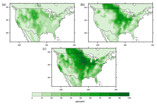
Figure 1.
Percentage of C3 non-arctic grasses (PFT 13 in CLM) (a), crops (PFT 15) (b), and their combination (c) over the contiguous US. PFT maps were derived from the 1-km IGBP (International Geosphere-Biosphere Program) DISCover dataset and the 1-km University of Maryland tree cover dataset [85]. This PFT product is modified by re-labeling the IGBP classes of the MODIS Land Cover Type 1 product. Red dots indicate FLUXNET station locations.
Over regions where crop and grass PFT percentage is low (such as the East Coast or Southwest), our GPP estimation approach may not be accurate since we have not formulated equations for other PFTs. Therefore, our primary objective is to investigate and evaluate the performance of MLR equations over the Great Plains and Texas. We principally focus on finding the relationships between SIF and GPP that are hypothesized to vary for different plant types and be pertinent to environmental conditions over a specific region.
3. Results
While SIF has a strong and highly linear relationship with GPP and has been previously used for its quantification without auxiliary data [22,27], it is necessary to ensure that no information useful for GPP quantification purposes is lost. In our case, one caveat can potentially stem from the relatively coarse spatial resolution of the datasets. It is to be noted that while changes in soil moisture and precipitation are already reflected in corresponding SIF signal fluctuations, it is possible that these parameters might not be well delineated by SIF due to its comparatively lower spatial resolution. Therefore, in order to provide substantiation for usage of a few predictor variables in addition to SIF, we have turned to the covariogram analysis.
The covariogram might be thought of as the covariance, i.e., similarity, of point values as a function of distance between the points, thus enabling an understanding of how important spatial variability is for each given variable. Over both the Great Plains (Figure 2a) and Texas (Figure 2b) soil moisture and GPP show a pattern of an almost linear reduction in covariance, i.e., the degree of similarity between the values of each variable at two given points becomes significantly lower as the distance between the points increases.
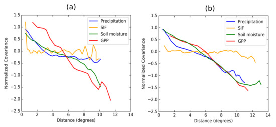
Figure 2.
Covariogram of SIF, precipitation, soil moisture, and GPP data over (a) the Great Plains and (b) Texas.
Contrastingly, SIF covariogram is represented by a relatively straight line, which is characterized by a greater number of smaller scale fluctuations. As can be inferred from Figure 2, SIF generally demonstrates less variability over the same spatial extent compared to precipitation, soil moisture, and GPP itself, at least in part due to the coarseness of the satellite SIF data. One important aspect in GPP and SIF relationship, as seen from the covariogram analysis, lies in the fact that GPP and SIF covariance changes do not go hand in hand, and GPP covariance trends are similar to those of precipitation and soil moisture, not SIF. Since spatial variability is more significant in GPP, using SIF that is less prone to variations over the same spatial domain might lead to larger errors in GPP values if they are predicted based solely on SIF.
Figure 3 demonstrates the lead–lag relationship between precipitation and SIF, soil moisture and precipitation, and SIF and soil moisture for US-Ne3 and US-KFS stations, respectively. It can be inferred that for US-Ne3 station with the dominant crop vegetation, the lag between precipitation and corresponding SIF is on the scale of 4 weeks (Figure 3a), while over US-KFS station, where grass is prevalent, this lag is about 2 weeks (Figure 3b). There is no significant lag between precipitation and soil moisture values for both US-Ne3 and US-KFS stations (Figure 3c,d), which is also expected. Similar temporal relationships between SIF, precipitation and soil moisture have also been found for the remaining FLUXNET stations used in this research (not shown).
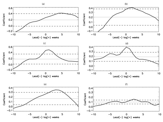
Figure 3.
Lead–lag correlation between SIF and precipitation (a,b), precipitation and soil moisture (c,d), and SIF and soil moisture (e,f) for US-Ne3 (a,c,e) and US-KFS (b,d,f) stations respectively. Dashed lines denote the 95% confidence level.
Figure 4 illustrates the temporal relationship between plant water, expressed as soil moisture index based on ESA soil moisture, and SIF data. The soil moisture index calculations are similar to those used in the parameterization scheme for soil moisture limitation to transpiration in land surface models, e.g., Noah-Multiparameterization Land Surface Model (Noah-MP LSM) [87]: when the index approaches 1, the plant water need reaches its maximum; when the index is equal to 0, the need is at its minimum. As can be inferred from Figure 4, water need has a peak towards mid June–end of July, which roughly coincides with the timing of pollination and kernel development in corn, and the beginning of pod development in soybean—the most important periods for corn and soy plants to have an adequate water supply. This peak in water need, as expressed by soil moisture index, is followed by a peak in SIF, which is indicative of high photosynthetic rates and potentially mass gain and GPP in crops by this later time in the growing season. NDVI generally follows a dynamic similar to that of SIF: both show a peak after the highest water need is noted. NDVI demonstrates a wider peak during the growth season, which is probably due to the difference in the temporal resolution of SIF and NDVI data products used in this study. These findings show that water availability at the developmental stage of plant lifecycle is likely to affect plant SIF and GPP at later stages: when a plant does not have enough water available to meet evapotranspiration demands during the late development stage (i.e., when a plant is typically most sensitive to water stress), this can lead to a significant reduction in plant production [40,88,89], which is reflected in SIF and GPP.
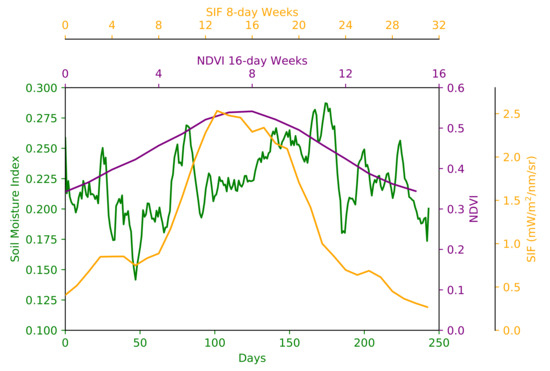
Figure 4.
Lead–lag relationship between SIF and plant water need based on soil moisture index calculated from ESA soil moisture data. Soil moisture index is calculated as , where is soil moisture value at any given day of the growing season, and are the highest and lowest soil moisture values during the growing season, respectively. The soil moisture index and SIF values are averaged over the study period of 2007–2012. Day 0 corresponds to April 1st, which is considered the beginning of the growing season. SIF, soil moisture and NDVI values are estimated from grids of size 0.5 × 0.5°, 0.25 × 0.25° and 1 × 1 km, respectively, surrounding US-Ne3 FLUXNET station (41.1797 °N, –96.4396 °E). US-Ne3 station has rotated crop assignments: soybean at even years and corn at odd years [90].
3.1. Assessing the Relationships between the Predictors for Different Vegetation Types
First, we looked into (1) how satellite-retrieved SIF itself correlates with GPP from ground-based flux tower stations. Then, as shown in Figure 5, Figure 6, Figure 7, Figure 8 and Figure 9, we estimated correlation and root-mean-square error (RMSE) for the following cases: (2) SIF-based GPP, (3) SIF- and precipitation-based GPP, (4) SIF-, precipitation- and soil-moisture-based GPP (i.e., MLR-based GPP). For the final case (5), we explored the SIF–precipitation–soil-moisture relationship using the lead–lag correlation analysis and its application for GPP quantification
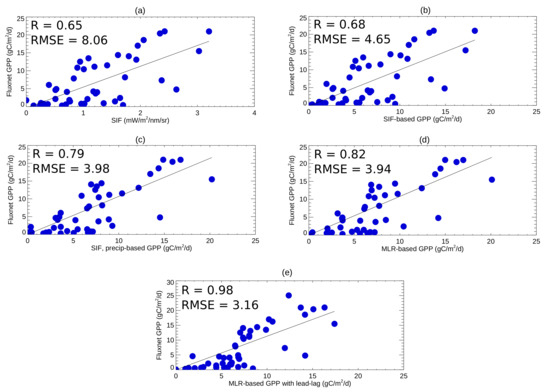
Figure 5.
Relationship of mean monthly GPP (gC/m/day) measured at FLUXNET stations with C3 crop vegetation (Table 1) used in this study and (a) GOME-2 SIF; (b) SIF-based GPP; (c) SIF- and precipitation-based GPP; (d) MLR-based GPP (SIF, precipitation, soil moisture as predictors); (e) MLR-based GPP with lead–lag. The Spearman’s correlation coefficient R and root-mean-square error (gC/m/day) are shown.
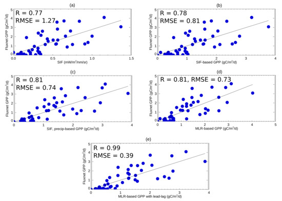
Figure 6.
Relationship of mean monthly GPP (gC/m/day) measured at FLUXNET stations with C3 non-arctic grass vegetation (Table 1) used in this study and (a) GOME-2 SIF; (b) SIF-based GPP; (c) SIF- and precipitation-based GPP; (d) MLR-based GPP (SIF, precipitation, soil moisture as predictors); (e) MLR-based GPP with lead–lag. The Spearman’s correlation coefficient R and root-mean-square error (gC/m/day) are shown.
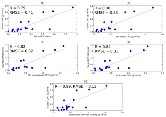
Figure 7.
Relationship of mean monthly GPP (gC/m/day) measured at FLUXNET stations with C4 grass vegetation (Table 1) used in this study and (a) GOME-2 SIF; (b) SIF-based GPP; (c) SIF- and precipitation-based GPP; (d) MLR-based GPP (SIF, precipitation, soil moisture as predictors); (e) MLR-based GPP with lead–lag. The Spearman’s correlation coefficient R and root-mean-square error (gC/m/day) are shown.
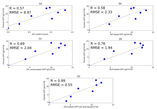
Figure 8.
Relationship of mean monthly GPP (gC/m/day) measured at US-Tw3 FLUXNET station characterized by alfalfa vegetation (Table 1) and (a) GOME-2 SIF; (b) SIF-based GPP; (c) SIF- and precipitation-based GPP; (d) MLR-based GPP (SIF, precipitation, soil moisture as predictors); (e) MLR-based GPP with lead–lag.The Spearman’s correlation coefficient R and root-mean-square error (gC/m/day) are shown.
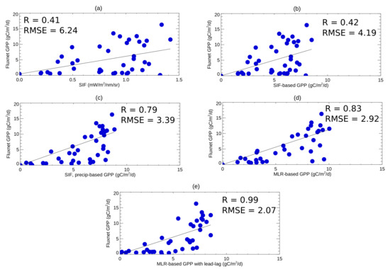
Figure 9.
Relationship of mean monthly GPP (gC/m/day) measured at US-Twt FLUXNET station with rice as a characteristic plant species (Table 1) and (a) GOME-2 SIF; (b) SIF-based GPP; (c) SIF- and precipitation-based GPP; (d) MLR-based GPP (SIF, precipitation, soil moisture as predictors); (e) MLR-based GPP with lead–lag. The Spearman’s correlation coefficient R and root-mean-square error (gC/m/day) are shown.
Figure 5 demonstrates correlation between GPP measured at the FLUXNET stations with C3 crop vegetation and GPP calculated with the use of the above-mentioned five combinations of predictors, over the entire vegetation period of a year, for 2007–2012. It can be noted that satellite SIF has a moderately strong relationship with FLUXNET GPP (Figure 5a), but the approach producing GPP estimates based on varying sets of predictors tends to yield better results, as expressed by improvements in the correlation coefficient R: e.g., from 0.65 when SIF connection to FLUXNET GPP is considered (Figure 5a) to 0.68 for the case when SIF-based GPP and FLUXNET GPP are used (Figure 5b). One curious feature is related to the existence of a “jump” in GPP quantification quality when precipitation data are taken into consideration: with the introduction of precipitation into MLR calculation, correlation coefficient R demonstrates an increase of 0.11 (from 0.68 to 0.79) as compared to the case using SIF data only (compare Figure 5b and Figure 5c); further addition of soil moisture leads to a relatively small increase in R (Figure 5d). However, the most significant rise in R is noted when the MLR equation is enhanced by the introduction of lead–lag: R increases from 0.82 to 0.98 (Figure 5e).
Figure 6 illustrates changes in the tightness of the correlation between FLUXNET GPP and C3 grass GPP calculated with the use of the same methods as in Figure 5. Similarly to Figure 5, calculated GPP estimates and FLUXNET GPP become more significantly correlated as the independent variables are introduced; it is also shown that, initially, the correlation between SIF and FLUXNET GPP without any ancillary data is relatively high (R = 0.77, Figure 6a) while that for the case of C3 crops was only 0.65 (Figure 5a). A similar pattern of increasing correlation and decreasing RMSE is also noted for C4 grasses (Figure 7a–e); the MLR-based equation with the inclusion of the lead–lag relationship yields the maximum correlation (R = 0.99) between estimated and FLUXNET GPP values. One can also notice that grass and crop vegetation cases exhibit a slightly different response to the addition of predictor variables: C3 non-arctic and C4 grasses GPP values demonstrate a rather monotonic increase in correlation with FLUXNET GPP, with small incremental steps, and one significant increase when lead–lag is considered (compare Figure 6a–d and Figure 6e; Figure 7a–d and Figure 7e). C3 crop vegetation GPP, on the other hand, is characterized by two significant correlation improvements: one when precipitation is introduced into GPP quantification (Figure 5c) and the other related to the addition of lead–lag (Figure 5e).
Overall, GPP estimates derived with the use of MLR while taking the lead–lag relationship into consideration are close to those from FLUXNET network: at the crop stations peak mean monthly GPP can be up to 20 gC/m/day, while for the grass sites mean monthly GPP does not exceed 10 gC/m/day. These findings agree well with those reported by Guanter et al. [22].
We have also explored how the inclusion of lead–lag into the relationship between predictors influences GPP estimates for individual plant species. Alfalfa and rice, both C3 crop species, cultivated at US-Tw3 and US-Twt stations, respectively, were selected for this purpose. Figure 8a and Figure 9a reveal that the correlation between SIF and flux tower GPP estimates demonstrates a moderate strength of relationship (0.57 and 0.41 for alfalfa and rice, respectively).
It can be seen that for the rice station, the addition of precipitation (compare Figure 9b and Figure 9c) into the GPP equations has played a substantial role in the improvement of the correlation between MLR GPP estimates and respective FLUXNET GPP values, while such a change in R is not noted for alfalfa vegetation. These results imply that the sensitivity of crop production to various environmental parameters such as precipitation is an essential factor to consider when investigating crop production. Moreover, it is necessary to analyze the interplay between such sensitivities: e.g., rice, which is often planted during the tropical rainy season, has a water demand of 450–700 mm/total growing season while alfalfa water need is about two times higher and comprises 800–1600 mm/total growing season. However, rice is known to be less drought-resistant than alfalfa [40] and also to be more significantly impacted by precipitation levels than other crops such as wheat and maize [91], which might explain why the addition of precipitation to the MLR GPP equation leads to the pronounced improvement in GPP estimates for rice but not for alfalfa.
Overall, as in the previous cases with C3/C4 grasses and C3 crops considered as a whole, GPP estimates for individual plant types demonstrate an analogous response to the introduction of more predictor variables: the correlation between predicted and observed GPP becomes more significant with the addition of predictors, and especially lead–lag connection.
It is apparent from our findings that knowledge of plant lifecycle, lead–lag relationships, and the sensitivity of different plants to various environmental parameters is crucial for the purpose of plant production quantification. In order to provide more support for the proposed framework aimed at better MLR GPP estimation, we have calculated mean values and errors for the predicted GPP (MLR equation with lead–lag), and the reference datasets, MOD17A2 and FLUXNET GPP, within the CLM grid box surrounding US-ARM, US-AR1 and US-AR2 stations. Figure 10 shows that our mean monthly (for JJA of all the years) total (grass and crops combined) GPP within the grid box (315 gC/m/month) is consistent with FLUXNET stations’ observations (394 gC/m/month). Although MODIS captures the drought trend, the observed values of GPP within the grid box surrounding the stations are only 123 gC/m/month. This shows that our predicted, i.e., MLR-based with lead–lag, GPP estimates are the closest to the actual plant production, as inferred from FLUXNET flux tower observations.
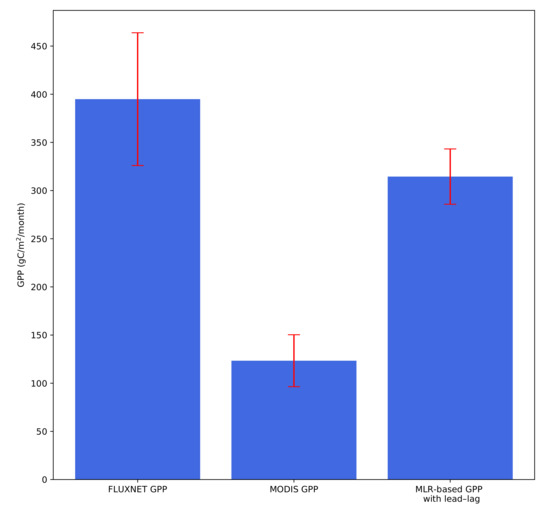
Figure 10.
Mean total GPP (gC/m/month) within a CLM grid box surrounding US-ARM, US-AR1 and US-AR2 stations in JJA 2007–2012. Total GPP is calculated as a sum of C3 non-arctic grass GPP, C4 grass GPP and C3 crop GPP.
3.2. Quantifying GPP over Texas and the Great Plains Using the Multiple Linear Regression Approach
Figure 11 and Figure 12 show total predicted GPP over Texas and the contiguous US, respectively. As mentioned in the data and methodology section, we have calculated GPP from the MLR equation using GOME-2 SIF, TRMM precipitation, and ESA CCI soil moisture data, with the inclusion of lead–lag relationship between SIF and precipitation. Figure 11 shows that predicted GPP over Texas (within 30–36 °N/95–105 °W grid box) in 2011 is significantly lower than that of 2007. The area with GPP values higher than 75 gC/m/month decreased significantly from 2007 to 2011, and specifically from June 2011 to August 2011, which is not typical for a normal yielding year. Figure 11d–f demonstrate that in 2011 drought conditions were limited to Texas as there was no significant change in GPP over the Great Plains (Figure 12d–f). These findings indicate that our MLR-based approach with lead–lag is able to capture the drought-related reduction in GPP over Texas in 2011.
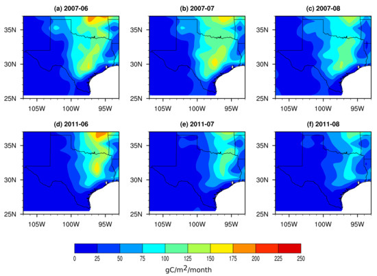
Figure 11.
Spatial patterns of monthly total (C3/C4 grass plus C3 crop) predicted GPP based on SIF, precipitation and soil moisture over Texas in summer 2007, chosen as reference year (a–c), and summer 2011—drought year in Texas) (d–f).
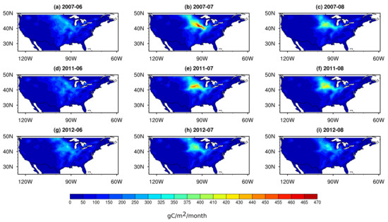
Figure 12.
Spatial patterns of monthly total (C3/C4 grass plus C3 crop) predicted GPP based on SIF, precipitation and soil moisture for summer 2007, chosen as reference year (a–c); summer 2011—drought year in Texas (d–f); and summer 2012—the Great Plains drought (g–i).
Figure 12 shows that maximum GPP values found over the Great Plains (Figure 12a–c) in the normal yielding year amount to 500 gC/m/month, which agrees well with FLUXNET data [22]. Predicted GPP indicates that 2012 was a severe drought year over the Great Plains as compared to 2007. The impact of the drought is clearly seen in 2012, as GPP decreased significantly compared to 2007 and 2011 (Figure 12g–h). Figure 11 and Figure 12 show that our predicted GPP estimates are capable of capturing the 2011 Texas drought effect and also the progression of the drought over the Great Plains region (along with Texas) in 2012. These results demonstrate the robustness of the approach presented in this research study, both in terms of the magnitude of GPP values and their trend.
We have also compared our results with MODIS observational reference data: Figure 13 shows that MODIS GPP values are about 50% lower than those of predicted gross primary production. GPP values based on MODIS satellite data range between 200 and 300 gC/m/month over the Great Plains. MODIS is able to detect a drought signal over the Great Plains in 2012 (Figure 13g–i) and Texas in 2011 (Figure 13d–f), as areas with GPP < 100 gC/m/month spread to the north and east, towards the Great Plains. MODIS observations also provide evidence of no reduction in GPP over the Great Plains in 2011, which is expected and also confirmed by monthly US Drought Monitor reports for JJA in 2011. Moreover, MODIS GPP over the Great Plains in August 2011 was higher than that in August 2007 and is consistent with the trend we observed in the predicted GPP (Figure 12c,f). Thus, our predicted GPP agrees well with MODIS GPP values in terms of capturing the drought conditions effect on plant production. Our MLR-based approach with lead–lag consideration can be used to provide GPP estimates that are more accurate in terms of absolute values than MODIS reference data.
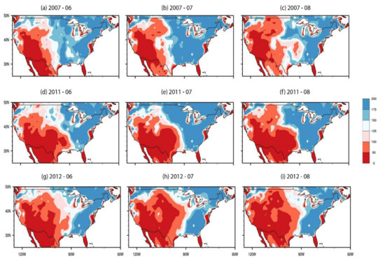
Figure 13.
Gross primary production (gC/m/month) from MOD17A2 data product in summer 2007 (a–c), summer 2011 (d–f), and summer 2012 (g–i).
Figure 14 indicates that BESS GPP values are typically lower than MLR GPP presented in this study and are slightly higher than MODIS GPP, which is likely related to the fact that the BESS algorithm considers the differences in C3/C4 photosynthetic pathways, while MODIS algorithm uses the same LUE across all vegetation types [92]. BESS is also capable of capturing the drought propagation in water stress years. It can be noted that in 2011 Texas experienced a significant decrease in GPP (below 100 gC/m/month), which is also noticeable in 2012. GPP over the Great Plains in 2012 demonstrated a decrease, which is especially pronounced in July–August 2012 as compared to 2007 and 2011 (Figure 14h,i).
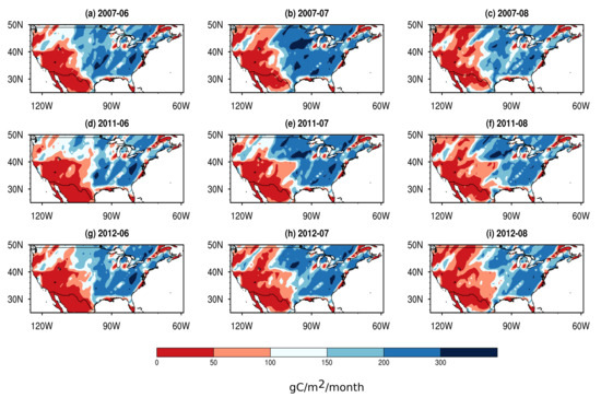
Figure 14.
Gross primary production (gC/m/month) from BESS data product in summer 2007 (a–c), summer 2011 (d–f), and summer 2012 (g–i).
FLUXNET GPP observations in a time series at select stations have also been included in the comparison (Figure 15). Oklahoma-based US-ARM, US-AR1 and US-AR2 stations show a characteristic decline in GPP over the second half of 2011 and recovery in 2012. US-Ne3 station located in Nebraska (central portion of the Great Plains) demonstrates an opposite pattern: an increase in GPP is noted in summer of 2011, with a decrease in summer 2012, which agrees well with the MLR GPP.
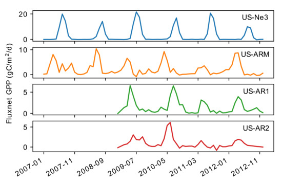
Figure 15.
Gross primary production (gC/m/day) over select FLUXNET stations in 2007–2012. More detailed information about the stations can be found in Table 1.
4. Discussion
This research study aims specifically at investigating how already existing satellite SIF products (on the example of GOME-2) can be complemented by other parameters, such as precipitation and soil moisture, in order to produce reasonable GPP estimates. To our knowledge, this is also the first study to quantitatively assess the lead–lag relationship between water availability in the critical plant development period and its reflection in GPP and SIF at later stages of the plant lifecycle. In this research, we have derived separate equations quantifying relationships between SIF and GPP based on the differences in grass and crop plant functional types and taking into account precipitation and soil moisture conditions over the contiguous US.
In this regard, a factor that has the potential to complicate the relationship between SIF itself and GPP is the sun-satellite view observation geometry, which could introduce unwanted variation in observational SIF and cause large uncertainties in the SIF–GPP relationship. He et al. [93] demonstrated that angular normalization of SIF by hot spot direction could improve the correlation between SIF and GPP by 0.04 ± 0.03–0.07 ± 0.04 on average, especially in deciduous broadleaf forests. The angular normalization as a prerequisite step in using satellite SIF products will be addressed in future studies.
We have used well established MODIS products as an observational reference along with more recent BESS data. Other newly available GPP products such as Vegetation Photosynthesis Model (VPM) [71] and FLUXCOM [94] can potentially serve as additional benchmarks for the evaluation of GPP estimates and might be useful for future research. Near-infrared reflectance of vegetation (NIRv, [95]) will also be used in future studies, as it has demonstrated a strong relationship with both measured and modeled GPP and mostly resolves the mixed-pixel problem arising from the need to disentangle the contribution of vegetation to the observed spectral signal in remotely sensed data.
We have performed GPP estimation and employed precipitation and soil moisture datasets pertinent to the contiguous US only. Similarly, as seen from this study, FLUXNET measurements from other regions such as Europe, East and Southeast Asia, South America can be used, depending on prevalent biome types, precipitation, and soil moisture content to establish such SIF–GPP relationships.
The lead–lag relationship discussed in this study is likely to differ for various biomes represented by different PFTs, as shown in our analysis. This fact is to be taken into account if similar research is to be conducted for vegetation that cannot be classified as crops or grasses. For example, deciduous trees might exhibit more resistance to drought conditions compared to crops due to their trunk water storage, which may result in a longer delay between precipitation and fluorescence levels. Hence, there might be a different lead–lag relationship between tree production and precipitation, which warrants further investigation.
Our findings indicate that SIF–GPP relationships tend to vary not only between vegetation types, but also between crop species specifically. This is reflected in a significant improvement in agreement between FLUXNET and predicted MLR GPP when precipitation is considered for rice, but not for alfalfa. These results imply that differing sensitivity of crop production to various environmental parameters such as precipitation is an important factor to be taken into account when examining and quantifying crop production.
It is also important to examine possible differences in GPP quantification related to the fact that most plants follow C3 or C4 photosynthetic pathways. For instance, C3 plants are expected to be more sensitive to precipitation than C4 vegetation [96]: such a differential plant response might need to be accounted for in further research focused on plant production, especially in the light of the global climate change, which might have implications for plant productivity.
5. Conclusions
In this study, we have modeled gross primary production with the use of solar-induced chlorophyll fluorescence, precipitation and soil moisture, while considering differences in grass and crop plant functional types over the contiguous US. Our results show that correlation (root-mean-square error) between the FLUXNET and modeled gross primary production increases (decreases) from 0.41 (8.97 gC/m/d) to 0.99 (0.13 gC/m/d) with the addition of extra parameters such as precipitation and soil moisture and inclusion of the lead–lag relationship. Mean monthly GPP values calculated for summers in 2007–2012 with the use of the multiple linear regression approach and lead–lag are comparable to the FLUXNET measurements, while reference MODIS and BESS datasets demonstrate a tendency to underestimate GPP by approximately 50%. GPP values calculated with the use of the MLR approach and lead–lag also capture the drought trends successfully and are consistent with the observational trends from MODIS and BESS. In 2011, modeled GPP over Texas is approximately 50–75 gC/m/month lower than in a normal yielding year of 2007; over the Great Plains, such a departure is comparable to that over Texas, as the area with production greater than 400 gC/m/month was reduced significantly in July and August 2012.
Our results demonstrate that GPP values based on various combinations of predictors, i.e., SIF, precipitation and soil moisture, have lower correlation coefficients and higher RMSE until and unless lead–lag relationship between the above mentioned predictors is considered. Since a plant is most vulnerable to water stress in its development period, we expect that plant production later in the season would depend on precipitation and soil moisture during the development stage. This study highlights the importance of water availability for plants during their development stage and its influence on plant production later in the season. It is also the first one to demonstrate that incorporation of plant physiological variations associated with water availability and demand at different stages of its lifetime can play an important role in estimation of plant production [97,98,99,100], especially under drought conditions that are likely to increase in frequency and severity in future.
This study further supports the claim that relationships between SIF and GPP are different for crops and grasses; using the statistically justified inclusion of regional precipitation and soil moisture, such relationships can be derived and used to improve GPP estimates.
Author Contributions
Conceptualization, M.H. and Z.-L.Y.; methodology, Z.-L.Y. and M.H.; formal analysis, M.H.; investigation, M.H.; resources, Z.-L.Y.; writing—original draft preparation, M.H.; writing—review and editing, M.H. and Z.-L.Y.; visualization, M.H.; supervision, Z.-L.Y.; funding acquisition, Z.-L.Y. All authors have read and agreed to the published version of the manuscript.
Funding
This study was supported by the National Key Research and Development Program of China (Grant No. 2016YFA0600403) and funds from Jackson School of Geosciences.
Acknowledgments
GOME-2 v25 level 3 SIF data are available at http://avdc.gsfc.nasa.gov. TRMM 3B42 and 3B43 products were obtained from https://mirador.gsfc.nasa.gov/. MODIS and FLUXNET GPP data are publicly available at https://lpdaac.usgs.gov/ and https://fluxnet.ornl.gov/, respectively. ESA CCI soil moisture products are provided by the European Space Agency at http://www.esa-soilmoisture-cci.org/. BESS GPP data can be accessed at http://environment.snu.ac.kr/bess_flux/.
Conflicts of Interest
The authors declare no conflict of interest.
Abbreviations
The following abbreviations are used in this manuscript:
| AMSR-E | Advanced Microwave Scanning Radiometer |
| APAR | absorbed photosynthetically active radiation |
| ASCAT | Advanced Scatterometer |
| BESS | Breathing Earth System Simulator |
| BPLUT | biome property look-up table |
| CLM | Community Land Model |
| ERS | European Remote Sensing |
| ESA CCI SM | European Space Agency Climate Change Initiative Soil Moisture |
| FPAR | fraction of absorbed photosynthetically active radiation |
| GOME-2 | Global Ozone Monitoring Experiment 2 |
| GPP | gross primary production |
| IGBP | International Geosphere-Biosphere Program |
| JJA | June, July, August |
| LAI | leaf area index |
| LUE | light use efficiency |
| MLR | multiple linear regression |
| MODIS | Moderate Resolution Imaging Spectroradiometer |
| MPI-BGC | Max Planck Institute for Biogeochemistry |
| NDVI | Normalized Difference Vegetation Index |
| NIRv | near-infrared reflectance of terrestrial vegetation |
| Noah-MP LSM | Noah-Multiparameterization Land Surface Model |
| NPP | net primary production |
| NPQ | non-photochemical quenching |
| PAR | photosynthetically active radiation |
| PFT | plant functional type |
| RMSE | root-mean-square error |
| SIF | solar-induced chlorophyll fluorescence |
| SMM/I | Special Sensor Microwave Imager |
| SMMR | Scanning Multichannel Microwave Radiometer |
| TMI | Tropical Rainfall Measuring Mission Microwave Imager |
| TRMM | Tropical Rainfall Measuring Mission |
| USDA | US Department of Agriculture |
| VPD | vapor pressure deficit |
| VPM | Vegetation Photosynthesis Model |
References
- Al-Kaisi, M.M.; Broner, I. Crop Water Use and Growth Stages; Colorado State University Extension: Fort Collins, CO, USA, 2009. [Google Scholar]
- Beer, C.; Reichstein, M.; Tomelleri, E.; Ciais, P.; Jung, M.; Carvalhais, N.; Rödenbeck, C.; Arain, M.A.; Baldocchi, D.; Bonan, G.B.; et al. Terrestrial gross carbon cioxide uptake: Global distribution and covariation with climate. Science 2010, 329, 834–838. [Google Scholar] [CrossRef] [PubMed]
- Running, S.W.; Nemani, R.R.; Heinsch, F.A.; Zhao, M.; Reeves, M.; Hashimoto, H. A continuous satellite-derived measure of global terrestrial primary production. BioScience 2004, 54, 547–560. [Google Scholar] [CrossRef]
- Friedlingstein, P.; Cox, P.; Betts, R.; Bopp, L.; von Bloh, W.; Brovkin, V.; Cadule, P.; Doney, S.; Eby, M.; Fung, I.; et al. Climate–carbon cycle feedback analysis: Results from the CMIP4 model intercomparison. J. Clim. 2006, 19, 3337–3353. [Google Scholar] [CrossRef]
- Sitch, S.; Huntingford, C.; Gedney, N.; Levy, P.E.; Lomas, M.; Piao, S.L.; Betts, R.; Ciais, P.; Cox, P.; Friedlingstein, P.; et al. Evaluation of the terrestrial carbon cycle, future plant geography and climate-carbon cycle feedbacks using five Dynamic Global Vegetation Models (DGVMs). Glob. Chang. Biol. 2008, 14, 2015–2039. [Google Scholar] [CrossRef]
- Sitch, S.; Smith, B.; Prentice, I.C.; Arneth, A.; Bondeau, A.; Cramer, W.; Kaplan, J.O.; Levis, S.; Lucht, W.; Sykes, M.T.; et al. Evaluation of ecosystem dynamics, plant geography and terrestrial carbon cycling in the LPJ dynamic global vegetation model. Glob. Chang. Biol. 2003, 9, 161–185. [Google Scholar] [CrossRef]
- Xu, M.; Hoffman, F. Evaluations of CMIP5 simulations over cropland. In Remote Sensing and Modeling of Ecosystems for Sustainability XII; International Society for Optics and Photonics: Bellingham, WA, USA, 2015; Volume 9610, p. 961003. [Google Scholar] [CrossRef]
- Cook, B.I.; Ault, T.R.; Smerdon, J.E. Unprecedented 21st century drought risk in the American Southwest and Central Plains. Sci. Adv. 2015, 1, e1400082. [Google Scholar] [CrossRef] [PubMed]
- Dai, A. Increasing drought under global warming in observations and models. Nat. Clim. Change 2013, 3, 52. [Google Scholar] [CrossRef]
- Sheffield, J.; Wood, E.F. Projected changes in drought occurrence under future global warming from multi-model, multi-scenario, IPCC AR4 simulations. Clim. Dyn. 2008, 31, 79–105. [Google Scholar] [CrossRef]
- Wang, G. Agricultural drought in a future climate: Results from 15 global climate models participating in the IPCC 4th assessment. Clim. Dyn. 2005, 25, 739–753. [Google Scholar] [CrossRef]
- Ciais, P.; Reichstein, M.; Viovy, N.; Granier, A.; Ogée, J.; Allard, V.; Aubinet, M.; Buchmann, N.; Bernhofer, C.; Carrara, A.; et al. Europe-wide reduction in primary productivity caused by the heat and drought in 2003. Nature 2005, 437, 529. [Google Scholar] [CrossRef]
- Zhao, M.; Running, S.W. Drought-induced reduction in global terrestrial net primary production from 2000 through 2009. Science 2010, 329, 940–943. [Google Scholar] [CrossRef] [PubMed]
- Liao, C.; Zhuang, Q. Reduction of global plant production due to droughts from 2001 to 2010: An analysis with a process-based global terrestrial ecosystem model. Earth Interact. 2015, 19, 1–21. [Google Scholar] [CrossRef]
- Krause, G.H.; Weis, E. Chlorophyll fluorescence and photosynthesis: The basics. Annu. Rev. Plant Physiol. Plant Mol. Biol. 1991, 42, 313–349. [Google Scholar] [CrossRef]
- Johnson, G.N.; Maxwell, K. Chlorophyll fluorescence—A practical guide. J. Exp. Bot. 2000, 51, 659–668. [Google Scholar] [CrossRef]
- Mohammed, G.H.; Colombo, R.; Middleton, E.M.; Rascher, U.; van der Tol, C.; Nedbal, L.; Goulas, Y.; Pérez-Priego, O.; Damm, A.; Meroni, M.; et al. Remote sensing of solar-induced chlorophyll fluorescence (SIF) in vegetation: 50 years of progress. Remote Sens. Environ. 2019, 231, 111177. [Google Scholar] [CrossRef]
- Meroni, M.; Rossini, M.; Guanter, L.; Alonso, L.; Rascher, U.; Colombo, R.; Moreno, J. Remote sensing of solar-induced chlorophyll fluorescence: Review of methods and applications. Remote Sens. Environ. 2009, 113, 2037–2051. [Google Scholar] [CrossRef]
- Kautsky, H.; Hirsch, A. Neue Versuche zur Kohlensäureassimilation. Naturwissenschaften 1931, 19, 964. [Google Scholar] [CrossRef]
- Kalaji, H.M.; Jajoo, A.; Oukarroum, A.; Brestic, M.; Zivcak, M.; Samborska, I.A.; Cetner, M.D.; ukasik, I.; Goltsev, V.; Ladle, R.J. Chlorophyll a fluorescence as a tool to monitor physiological status of plants under abiotic stress conditions. Acta Physiol. Plant. 2016, 38, 102. [Google Scholar] [CrossRef]
- Frankenberg, C.; Berry, J. Solar Induced Chlorophyll Fluorescence: Origins, Relation to Photosynthesis and Retrieval. In Comprehensive Remote Sensing; Elsevier: Amsterdam, The Netherlands, 2018; Volume 3, pp. 143–162. [Google Scholar] [CrossRef]
- Guanter, L.; Zhang, Y.; Jung, M.; Joiner, J.; Voigt, M.; Berry, J.A.; Frankenberg, C.; Huete, A.R.; Zarco-Tejada, P.; Lee, J.E.; et al. Global and time-resolved monitoring of crop photosynthesis with chlorophyll fluorescence. Proc. Natl. Acad. Sci. USA 2014, 111, E1327–E1333. [Google Scholar] [CrossRef]
- Frankenberg, C.; Fisher, J.B.; Worden, J.; Badgley, G.; Saatchi, S.S.; Lee, J.E.; Toon, G.C.; Butz, A.; Jung, M.; Kuze, A.; et al. New global observations of the terrestrial carbon cycle from GOSAT: Patterns of plant fluorescence with gross primary productivity. Geophys. Res. Lett. 2011, 38, L17706. [Google Scholar] [CrossRef]
- Meroni, M.; Picchi, V.; Rossini, M.; Cogliati, S.; Panigada, C.; Nali, C.; Lorenzini, G.; Colombo, R. Leaf level early assessment of ozone injuries by passive fluorescence and photochemical reflectance index. Int. J. Remote Sens. 2008, 29, 5409–5422. [Google Scholar] [CrossRef]
- Guanter, L.; Frankenberg, C.; Dudhia, A.; Lewis, P.E.; Gómez-Dans, J.; Kuze, A.; Suto, H.; Grainger, R.G. Retrieval and global assessment of terrestrial chlorophyll fluorescence from GOSAT space measurements. Remote Sens. Environ. 2012, 121, 236–251. [Google Scholar] [CrossRef]
- Damm, A.; Elbers, J.; Erler, A.; Gioli, B.; Hamdi, K.; Hutjes, R.; Kosvancova, M.; Meroni, M.; Miglietta, F.; Moersch, A.; et al. Remote sensing of sun-induced fluorescence to improve modeling of diurnal courses of gross primary production (GPP). Glob. Chang. Biol. 2010, 16, 171–186. [Google Scholar] [CrossRef]
- Guan, K.; Berry, J.A.; Zhang, Y.; Joiner, J.; Guanter, L.; Badgley, G.; Lobell, D.B. Improving the monitoring of crop productivity using spaceborne solar-induced fluorescence. Glob. Chang. Biol. 2016, 22, 716–726. [Google Scholar] [CrossRef]
- Wagner, W.; Hahn, S.; Gruber, A.; Dorigo, W. Identification of soil moisture retrieval errors: Learning from the comparison of SMOS and ASCAT. In Proceedings of the 2012 IEEE International Geoscience and Remote Sensing Symposium, Munich, Germany, 22–27 July 2012; pp. 3795–3798. [Google Scholar] [CrossRef]
- Porcar-Castell, A.; Atherton, J.; Tyystjärvi, E.; van der Tol, C.; Flexas, J.; Pfündel, E.E.; Moreno, J.; Frankenberg, C.; Berry, J.A. Linking chlorophyll a fluorescence to photosynthesis for remote sensing applications: Mechanisms and challenges. J. Exp. Bot. 2014, 65, 4065–4095. [Google Scholar] [CrossRef] [PubMed]
- Cui, T.; Sun, R.; Qiao, C. Assessing the factors determining the relationship between solar-induced chlorophyll fluorescence and GPP. In Proceedings of the 2016 IEEE International Geoscience and Remote Sensing Symposium, Beijing, China, 10–15 July 2016; pp. 3520–3523. [Google Scholar] [CrossRef]
- Verma, M.; Schimel, D.; Evans, B.; Frankenberg, C.; Beringer, J.; Drewry, D.T.; Magney, T.; Marang, I.; Hutley, L.; Moore, C.; et al. Effect of environmental conditions on the relationship between solar-induced fluorescence and gross primary productivity at an OzFlux grassland site. J. Geophys. Res. Biogeosci. 2017, 122, 716–733. [Google Scholar] [CrossRef]
- Churkina, G.; Running, S.W. Contrasting climatic controls on the estimated productivity of global terrestrial biomes. Ecosystems 1998, 1, 206–215. [Google Scholar] [CrossRef]
- Nemani, R.R.; Keeling, C.D.; Hashimoto, H.; Jolly, W.M.; Piper, S.C.; Tucker, C.J.; Myneni, R.B.; Running, S.W. Climate-driven increases in global terrestrial net primary production from 1982 to 1999. Science 2003, 300, 1560–1563. [Google Scholar] [CrossRef]
- Baker, N.R. Chlorophyll fluorescence: A probe of photosynthesis in vivo. Annu. Rev. Plant Biol. 2008, 59, 89–113. [Google Scholar] [CrossRef]
- Sun, K.; Liu, X.; Nowlan, C.R.; Cai, Z.; Chance, K.; Frankenberg, C.; Lee, R.A.M.; Pollock, R.; Rosenberg, R.; Crisp, D. Characterization of the OCO-2 instrument line shape functions using on-orbit solar measurements. Atmos. Meas. Tech. 2017, 10, 939–953. [Google Scholar] [CrossRef]
- Cendrero-Mateo, M.P.; Carmo-Silva, A.E.; Porcar-Castell, A.; Hamerlynck, E.P.; Papuga, S.A.; Moran, M.S. Dynamic response of plant chlorophyll fluorescence to light, water and nutrient availability. Funct. Plant Biol. 2015, 42, 746–757. [Google Scholar] [CrossRef] [PubMed]
- Liu, L.; Teng, Y.; Wu, J.; Zhao, W.; Liu, S.; Shen, Q. Soil water deficit promotes the effect of atmospheric water deficit on solar-induced chlorophyll fluorescence. Sci. Total Environ. 2020, 720, 137408. [Google Scholar] [CrossRef] [PubMed]
- Jiao, W.; Chang, Q.; Wang, L. The sensitivity of satellite solar-induced chlorophyll fluorescence to meteorological drought. Earths Future 2019, 7, 558–573. [Google Scholar] [CrossRef]
- Qiu, B.; Xue, Y.; Fisher, J.B.; Guo, W.; Berry, J.A.; Zhang, Y. Satellite chlorophyll fluorescence and soil moisture observations lead to advances in the predictive understanding of global terrestrial coupled carbon-water cycles. Glob. Biogeochem. Cycles 2018, 32, 360–375. [Google Scholar] [CrossRef]
- Brouwer, C.; Heibloem, M. Irrigation Water Management: Irrigation Water Needs; FAO: Rome, Italy, 1986; Volume 3. [Google Scholar]
- Morrison, M.; McLaughlin, N.; Cober, E.; Butler, G. When is short-season soybean most susceptible to water stress? Can. J. Plant Sci. 2006, 86, 1327–1331. [Google Scholar] [CrossRef]
- Doss, B.; Pearson, R.; Rogers, H.T. Effect of soil water stress at various growth stages on soybean yield. Agron J. 1974, 66, 297–299. [Google Scholar] [CrossRef]
- Dyer, J.M. Revisiting the deciduous forests of Eastern North America. BioScience 2006, 56, 341–352. [Google Scholar] [CrossRef]
- Mao, J.F.; Thornton, P.E.; Shi, X.Y.; Zhao, M.S.; Post, W.M. Remote sensing evaluation of CLM4 GPP for the period 2000-09. J. Clim. 2012, 25, 5327–5342. [Google Scholar] [CrossRef]
- Joiner, J.; Guanter, L.; Lindstrot, R.; Voigt, M.; Vasilkov, A.P.; Middleton, E.M.; Huemmrich, K.F.; Yoshida, Y.; Frankenberg, C. Global monitoring of terrestrial chlorophyll fluorescence from moderate-spectral-resolution near-infrared satellite measurements: Methodology, simulations, and application to GOME-2. Atmos. Meas. Tech. 2013, 6, 2803–2823. [Google Scholar] [CrossRef]
- Joiner, J.; Yoshida, Y.; Vasilkov, A.; Schaefer, K.; Jung, M.; Guanter, L.; Zhang, Y.; Garrity, S.; Middleton, E.; Huemmrich, K.; et al. The seasonal cycle of satellite chlorophyll fluorescence observations and its relationship to vegetation phenology and ecosystem atmosphere carbon exchange. Remote Sens. Environ. 2014, 152, 375–391. [Google Scholar] [CrossRef]
- Sun, Y.; Fu, R.; Dickinson, R.; Joiner, J.; Frankenberg, C.; Gu, L.; Xia, Y.; Fernando, N. Drought onset mechanisms revealed by satellite solar-induced chlorophyll fluorescence: Insights from two contrasting extreme events. J. Geophys. Res. Biogeosci. 2015, 120, 2427–2440. [Google Scholar] [CrossRef]
- Walther, S.; Voigt, M.; Thum, T.; Gonsamo, A.; Zhang, Y.; Köhler, P.; Jung, M.; Varlagin, A.; Guanter, L. Satellite chlorophyll fluorescence measurements reveal large-scale decoupling of photosynthesis and greenness dynamics in boreal evergreen forests. Glob. Chang. Biol. 2016, 22, 2979–2996. [Google Scholar] [CrossRef] [PubMed]
- Yang, X.; Tang, J.; Mustard, J.F.; Lee, J.E.; Rossini, M.; Joiner, J.; Munger, J.W.; Kornfeld, A.; Richardson, A.D. Solar-induced chlorophyll fluorescence that correlates with canopy photosynthesis on diurnal and seasonal scales in a temperate deciduous forest. Geophys. Res. Lett. 2015, 42, 2977–2987. [Google Scholar] [CrossRef]
- Dorigo, W.; de Jeu, R.; Chung, D.; Parinussa, R.; Liu, Y.; Wagner, W.; Fernández-Prieto, D. Evaluating global trends (1988–2010) in harmonized multi-satellite surface soil moisture. Geophys. Res. Lett. 2012, 39. [Google Scholar] [CrossRef]
- Hirschi, M.; Mueller, B.; Dorigo, W.; Seneviratne, S. Using remotely sensed soil moisture for land–atmosphere coupling diagnostics: The role of surface vs. root-zone soil moisture variability. Remote Sens. Environ. 2014, 154, 246–252. [Google Scholar] [CrossRef]
- Nicolai-Shaw, N.; Hirschi, M.; Mittelbach, H.; Seneviratne, S.I. Spatial representativeness of soil moisture using in situ, remote sensing, and land reanalysis data. J. Geophys. Res. Atmos. 2015, 120, 9955–9964. [Google Scholar] [CrossRef]
- Pratola, C.; Barrett, B.; Gruber, A.; Dwyer, E. Quality assessment of the CCI ECV soil moisture product using ENVISAT ASAR wide swath data over Spain, Ireland and Finland. Remote Sens. 2015, 7, 15388–15423. [Google Scholar] [CrossRef]
- Pratola, C.; Barrett, B.; Gruber, A.; Kiely, G.; Dwyer, E. Evaluation of a global soil moisture product from finer spatial resolution SAR data and ground measurements at Irish sites. Remote Sens. 2014, 6, 8190–8219. [Google Scholar] [CrossRef]
- Falge, E.; Baldocchi, D.; Tenhunen, J.; Aubinet, M.; Bakwin, P.; Berbigier, P.; Bernhofer, C.; Burba, G.; Clement, R.; Davis, K.J.; et al. Seasonality of ecosystem respiration and gross primary production as derived from FLUXNET measurements. Agric. For. Meteorol. 2002, 113, 53–74. [Google Scholar] [CrossRef]
- Falge, E.; Tenhunen, J.; Baldocchi, D.; Aubinet, M.; Bakwin, P.; Berbigier, P.; Bernhofer, C.; Bonnefond, J.M.; Burba, G.; Clement, R.; et al. Phase and amplitude of ecosystem carbon release and uptake potentials as derived from FLUXNET measurements. Agric. For. Meteorol. 2002, 113, 75–95. [Google Scholar] [CrossRef]
- Jung, M.; Reichstein, M.; Margolis, H.A.; Cescatti, A.; Richardson, A.D.; Arain, M.A.; Arneth, A.; Bernhofer, C.; Bonal, D.; Chen, J.; et al. Global patterns of land-atmosphere fluxes of carbon dioxide, latent heat, and sensible heat derived from eddy covariance, satellite, and meteorological observations. J. Geophys. Res. Biogeosci. 2011, 116. [Google Scholar] [CrossRef]
- Schwalm, C.R.; Williams, C.A.; Schaefer, K.; Arneth, A.; Bonal, D.; Buchmann, N.; Chen, J.; Law, B.E.; Lindroth, A.; Luyssaert, S.; et al. Assimilation exceeds respiration sensitivity to drought: A FLUXNET synthesis. Glob. Chang. Biol. 2010, 16, 657–670. [Google Scholar] [CrossRef]
- Zhao, F.; Dai, X.; Verhoef, W.; Guo, Y.; van der Tol, C.; Li, Y.; Huang, Y. FluorWPS: A Monte Carlo ray-tracing model to compute sun-induced chlorophyll fluorescence of three-dimensional canopy. Remote Sens. Environ. 2016, 187, 385–399. [Google Scholar] [CrossRef]
- Baldocchi, D.D. Assessing the eddy covariance technique for evaluating carbon dioxide exchange rates of ecosystems: Past, present and future. Glob. Chang. Biol. 2003, 9, 479–492. [Google Scholar] [CrossRef]
- Zhao, M.; Heinsch, F.A.; Nemani, R.R.; Running, S.W. Improvements of the MODIS terrestrial gross and net primary production global data set. Remote Sens. Environ. 2005, 95, 164–176. [Google Scholar] [CrossRef]
- Monteith, J.L. Solar radiation and productivity in tropical ecosystems. J. Appl. Ecol. 1972, 9, 747–766. [Google Scholar] [CrossRef]
- Gitelson, A.; Peng, Y.; Masek, J.; Rundquist, D.; Verma, S.; Suyker, A.; Baker, J.; Hatfield, J.; Meyers, T. Remote estimation of crop gross primary production with Landsat data. Remote Sens. Environ. 2012, 121, 404–414. [Google Scholar] [CrossRef]
- Heinsch, F.; Zhao, M.; Running, S.; Kimball, J.; Nemani, R.; Davis, K.; Bolstad, P.; Cook, B.; Desai, A.; Ricciuto, D.; et al. Evaluation of remote sensing based terrestrial productivity from MODIS using regional tower eddy flux network observations. IEEE Trans. Geosci. Remote Sens. 2006, 44, 1908–1923. [Google Scholar] [CrossRef]
- Turner, D.P.; Ritts, W.D.; Cohen, W.B.; Maeirsperger, T.K.; Gower, S.T.; Kirschbaum, A.A.; Running, S.W.; Zhao, M.; Wofsy, S.C.; Dunn, A.L.; et al. Site-level evaluation of satellite-based global terrestrial gross primary production and net primary production monitoring. Glob. Chang. Biol. 2005, 11, 666–684. [Google Scholar] [CrossRef]
- Turner, D.P.; Ritts, W.D.; Zhao, M.; Kurc, S.A.; Dunn, A.L.; Wofsy, S.C.; Small, E.E.; Running, S.W. Assessing interannual variation in MODIS-based estimates of gross primary production. IEEE Trans. Geosci. Remote Sens. 2006, 44, 1899–1907. [Google Scholar] [CrossRef]
- Wagle, P.; Xiao, X.; Suyker, A.E. Estimation and analysis of gross primary production of soybean under various management practices and drought conditions. ISPRS J. Photogramm. Remote Sens. 2015, 99, 70–83. [Google Scholar] [CrossRef]
- Wagle, P.; Zhang, Y.; Jin, C.; Xiao, X. Comparison of solar-induced chlorophyll fluorescence, light-use efficiency, and process-based GPP models in maize. Ecol. Appl. 2016, 26, 1211–1222. [Google Scholar] [CrossRef] [PubMed]
- Zhu, H.; Lin, A.; Wang, L.; Xia, Y.; Zou, L. Evaluation of MODIS gross primary production across multiple biomes in China using eddy covariance flux data. Remote Sens. 2016, 8, 395. [Google Scholar] [CrossRef]
- Wagle, P.; Xiao, X.; Torn, M.S.; Cook, D.R.; Matamala, R.; Fischer, M.L.; Jin, C.; Dong, J.; Biradar, C. Sensitivity of vegetation indices and gross primary production of tallgrass prairie to severe drought. Remote Sens. Environ. 2014, 152, 1–14. [Google Scholar] [CrossRef]
- Zhang, Y.; Xiao, X.; Wu, X.; Zhou, S.; Zhang, G.; Qin, Y.; Dong, J. A global moderate resolution dataset of terrestrial gross primary production for 2000–2016. Sci. Data 2017, 4, 170165. [Google Scholar] [CrossRef]
- Ryu, Y.; Baldocchi, D.D.; Kobayashi, H.; van Ingen, C.; Li, J.; Black, T.A.; Beringer, J.; Van Gorsel, E.; Knohl, A.; Law, B.E.; et al. Integration of MODIS land and atmosphere products with a coupled-process model to estimate gross primary productivity and evapotranspiration from 1 km to global scales. Glob. Biogeochem. Cycles 2011, 25, GB4017. [Google Scholar] [CrossRef]
- Jiang, C.; Ryu, Y. Multi-scale evaluation of global gross primary productivity and evapotranspiration products derived from Breathing Earth System Simulator (BESS). Remote Sens. Environ. 2016, 186, 528–547. [Google Scholar] [CrossRef]
- Huete, A.; Justice, C.; Liu, H. Development of vegetation and soil indices for MODIS-EOS. Remote Sens. Environ. 1994, 49, 224–234. [Google Scholar] [CrossRef]
- Justice, C.O.; Eck, T.; Tanré, D.; Holben, B.N. The effect of water vapour on the normalized difference vegetation index derived for the Sahelian region from NOAA AVHRR data. Int. J. Remote Sens. 1991, 12, 1165–1187. [Google Scholar] [CrossRef]
- Running, S.W.; Nemani, R.R. Relating seasonal patterns of the AVHRR vegetation index to simulated photosynthesis and transpiration of forests in different climates. Remote Sens. Environ. 1988, 24, 347–367. [Google Scholar] [CrossRef]
- Tucker, C.J.; Sellers, P.J. Satellite remote sensing of primary production. Int. J. Remote Sens. 1986, 7, 1395–1416. [Google Scholar] [CrossRef]
- Xu, C.; Li, Y.; Hu, J.; Yang, X.; Sheng, S.; Liu, M. Evaluating the difference between the normalized difference vegetation index and net primary productivity as the indicators of vegetation vigor assessment at landscape scale. Environ. Monit. Assess. 2012, 184, 1275–1286. [Google Scholar] [CrossRef] [PubMed]
- Faurtyot, T.; Baret, F. Vegetation water and dry matter contents estimated from top-of-the-atmosphere reflectance data: A simulation study. Remote Sens. Environ. 1997, 61, 34–45. [Google Scholar] [CrossRef]
- Soukharev, B.E.; Hood, L.L. Solar cycle variation of stratospheric ozone: Multiple regression analysis of long-term satellite data sets and comparisons with models. J. Geophys. Res. Atmos. 2006, 111. [Google Scholar] [CrossRef]
- Chakraborty, S.; Fu, R.; Wright, J.S.; Massie, S.T. Relationships between convective structure and transport of aerosols to the upper troposphere deduced from satellite observations. J. Geophys. Res. Atmos. 2015, 120, 6515–6536. [Google Scholar] [CrossRef]
- Garofalo, G.; Palermo, S.; Principato, F.; Theodosiou, T.; Piro, P. The influence of hydrologic parameters on the hydraulic efficiency of an extensive green roof in Mediterranean area. Water 2016, 8, 44. [Google Scholar] [CrossRef]
- Damm, A.; Guanter, L.; Paul-Limoges, E.; van der Tol, C.; Hueni, A.; Buchmann, N.; Eugster, W.; Ammann, C.; Schaepman, M. Far-red sun-induced chlorophyll fluorescence shows ecosystem-specific relationships to gross primary production: An assessment based on observational and modeling approaches. Remote Sens. Environ. 2015, 166, 91–105. [Google Scholar] [CrossRef]
- Oleson, K.W.; Lawrence, D.M.; Gordon, B.; Flanner, M.G.; Kluzek, E.; Peter, J.; Levis, S.; Swenson, S.C.; Thornton, E.; Feddema, J.; et al. Technical Description of Version 4.0 of the Community Land Model (CLM); No. NCAR/TN-478+STR; University Corporation for Atmospheric Research: Boulder, CO, USA, 2010. [Google Scholar] [CrossRef]
- Bonan, G.B.; Levis, S.; Kergoat, L.; Oleson, K.W. Landscapes as patches of plant functional types: An integrating concept for climate and ecosystem models. Glob. Biogeochem. Cycles 2002, 16. [Google Scholar] [CrossRef]
- Mena-Petite, A.; González-Moro, B.; González-Murua, C.; Lacuesta, M.; Rueda, A.M. Sequential effects of acidic precipitation and drought on photosynthesis and chlorophyll fluorescence parameters of Pinus Radiata D. Don Seedlings. J. Plant Physiol. 2000, 156, 84–92. [Google Scholar] [CrossRef]
- Niu, G.Y.; Yang, Z.L.; Mitchell, K.E.; Chen, F.; Ek, M.B.; Barlage, M.; Kumar, A.; Manning, K.; Niyogi, D.; Rosero, E.; et al. The community Noah land surface model with multiparameterization options (Noah-MP): 1. Model description and evaluation with local-scale measurements. J. Geophys. Res. Atmos. 2011, 116, D12109. [Google Scholar] [CrossRef]
- Kranz, W.L.; Irmak, S.; Van Donk, S.J.; Yonts, C.D.; Martin, D.L. Irrigation Management for Corn. In Neb Guide G1850; University of Nebraska: Lincoln, NE, USA, 2008; Volume 10, pp. 1–8. [Google Scholar]
- Hashim, M.; Siam, N.; Al-Dosari, A.; Asl-Gaadi, K.; Patil, V.; Tola, E.; Rangaswamy, M.; Samdani, M. Determination of water requirement and crop water productivity of crops grown in the Makkah region of Saudi Arabia. Aust. J. Basic Appl. Sci. 2012, 6, 196–206. [Google Scholar]
- Suyker, A.E.; Verma, S.B.; Burba, G.G.; Arkebauer, T.J. Gross primary production and ecosystem respiration of irrigated maize and irrigated soybean during a growing season. Agric. For. Meteorol. 2005, 131, 180–190. [Google Scholar] [CrossRef]
- Lobell, D.B.; Field, C.B. Global scale climate–crop yield relationships and the impacts of recent warming. Environ. Res. Lett. 2007, 2, 014002. [Google Scholar] [CrossRef]
- Chen, Y.; Gu, H.; Wang, M.; Gu, Q.; Ding, Z.; Ma, M.; Liu, R.; Tang, X. Contrasting performance of the remotely-derived GPP products over different climate zones across China. Remote Sens. 2019, 11, 1855. [Google Scholar] [CrossRef]
- He, L.; Chen, J.M.; Liu, J.; Mo, G.; Joiner, J. Angular normalization of GOME-2 sun-induced chlorophyll fluorescence observation as a better proxy of vegetation productivity. Geophys. Res. Lett. 2017, 44, 5691–5699. [Google Scholar] [CrossRef]
- Jung, M.; Reichstein, M.; Schwalm, C.; Huntingford, C.; Sitch, S.; Ahlström, A.; Arneth, A.; Camps-Valls, G.; Ciais, P.; Friedlingstein, P.; et al. Compensatory water effects link yearly global land CO2 sink changes to temperature. Nature 2017, 541, 516–520. [Google Scholar] [CrossRef]
- Badgley, G.; Field, C.B.; Berry, J.A. Canopy near-infrared reflectance and terrestrial photosynthesis. Sci. Adv. 2017, 3, e1602244. [Google Scholar] [CrossRef]
- Bi, Y.; Xie, H. C3 vegetation mapping and CO2 fertilization effect in the arid lower Heihe river basin, Northwestern China. Remote Sens. 2015, 7, 16384–16397. [Google Scholar] [CrossRef]
- Hsiao, T.; Fereres, E.; Acevedo, E.; Henderson, D. Water Stress and Dynamics of Growth and Yield of Crop Plants. In Water and Plant Life; Springer: Berlin/Heidelberg, Germany, 1976; pp. 281–305. [Google Scholar] [CrossRef]
- Osakabe, Y.; Osakabe, K.; Shinozaki, K.; Tran, L.S.P. Response of plants to water stress. Front. Plant Sci. 2014, 5, 86. [Google Scholar] [CrossRef]
- Fahad, S.; Bajwa, A.A.; Nazir, U.; Anjum, S.A.; Farooq, A.; Zohaib, A.; Sadia, S.; Nasim, W.; Adkins, S.; Saud, S.; et al. Crop production under drought and heat stress: Plant responses and management options. Front. Plant Sci. 2017, 8, 1147. [Google Scholar] [CrossRef]
- Sah, R.; Chakraborty, M.; Prasad, K.; Pandit, M.; Tudu, V.; Chakravarty, M.; Narayan, S.; Rana, M.; Moharana, D. Impact of water deficit stress in maize: Phenology and yield components. Sci. Rep. 2020, 10, 2944. [Google Scholar] [CrossRef] [PubMed]
Publisher’s Note: MDPI stays neutral with regard to jurisdictional claims in published maps and institutional affiliations. |
© 2020 by the authors. Licensee MDPI, Basel, Switzerland. This article is an open access article distributed under the terms and conditions of the Creative Commons Attribution (CC BY) license (http://creativecommons.org/licenses/by/4.0/).