Article

Accuracy Assessment and Correction of SRTM DEM Using ICESat/GLAS Data under Data Coregistration

1
Key Laboratory of Geomatics and Digital Technology of Shandong Province, Shandong University of Science and Technology, Qingdao 266590, China
2
College of Geodesy and Geomatics, Shandong University of Science and Technology, Qingdao 266590, China
*
Author to whom correspondence should be addressed.
Remote Sens. 2020, 12(20), 3435; https://doi.org/10.3390/rs12203435
Submission received: 5 September 2020 / Revised: 13 October 2020 / Accepted: 18 October 2020 / Published: 19 October 2020

Abstract

:
Shuttle Radar Topography Mission (SRTM) digital elevation model (DEM) inherently suffers from various errors. Many previous works employed Geoscience Laser Altimeter System onboard the Ice, Cloud, and land Elevation Satellite (ICESat/GLAS) data to assess and enhance SRTM DEM accuracy. Nevertheless, data coregistration between the two datasets was commonly neglected in their studies. In this paper, an automated and simple three dimensional (3D) coregistration method (3CM) was introduced to align the 3-arc-second SRTM (SRTM3) DEM and ICESat/GLAS data over Jiangxi province, China. Then, accuracy evaluation of the SRTM3 DEM using ICESat/GLAS data with and without data coregistration was performed on different classes of terrain factors and different land uses, with the purpose of evaluating the importance of data coregistration. Results show that after data coregistration, the root mean square error (RMSE) and mean bias of the SRTM3 DEM are reduced by 14.4% and 97.1%, respectively. Without data coregistration, terrain aspects with a sine-like shape are strongly related to SRTM3 DEM errors; nevertheless, this relationship disappears after data coregistration. Among the six land uses, SRTM3 DEM produces the lowest accuracy in forest areas. Finally, by incorporating land uses, terrain factors and ICESat/GLAS data into the correction models, the SRTM3 DEM was enhanced using multiple linear regression (MLR), back propagation neural network (BPNN), generalized regression NN (GRNN), and random forest (RF), respectively. Results exhibit that the four enhancement models with data coregistration obviously outperform themselves without the coregistration. Among the four models, RF produces the best result, and its RMSE is about 3.1%, 2.7% and 11.3% lower than those of MLR, BPNN, and GRNN, respectively. Moreover, 146 Global Navigation Satellite System (GNSS) points over Ganzhou city of Jiangxi province were used to assess the accuracy of the RF-derived SRTM3 DEM. It is found that the DEM quality is improved and has a similar error magnitude to that relative to the ICESat/GLASS data.

Graphical Abstract

1. Introduction

Digital elevation models (DEMs) are an indispensable input variable for geomorphological, hydrological, and ecological models in the applications, such as landslide detection [1], forest inventory [2] and flood hazard assessment [3]. The data source of DEMs includes field surveys, topographical maps, and remote sensing techniques [4,5]. At present, the remote-sensing-based techniques show significant advantages for producing high-accuracy and global-scale DEMs [6].
To date, DEMs with the most widespread use in geosciences were collected from the Shuttle Radar Topography Mission (SRTM) based on Interferometric Synthetic Aperture Radar (InSAR) technique [7]. Like other spatial datasets, SRTM DEM intrinsically contains various errors, which are associated with data acquisition sensors, measurement conditions on the ground and post-processing methodology [8]. With respect to spatial scale, the random component of SRTM DEM errors can be classified into speckle noise of short-wavelength (a few pixels), stripe noise of medium-wavelength (500 m–50 km) and absolute biases of long-wavelength (>20 km) [9,10]. SRTM DEM also suffers from systematic positive biases caused by vegetation canopy in forested areas [11]. Global assessment of SRTM DEM indicates that the magnitude of each height error component can reach to 10 m for 90% of the data [9]. These errors have a seriously negative impact on the success of SRTM DEM-related applications [12,13,14]. Thus, it is urgent to understand the spatial structure of SRTM DEM errors and then eliminate them to the greatest extent.
The accuracy of SRTM DEM has been fully assessed over different countries of the world. This is generally achieved by comparing SRTM DEM with high-quality DEMs [8,15,16,17] or high-accuracy ground control points (GCPs) collected by Global Navigation Satellite System (GNSS) [9,18,19,20,21,22]. However, field GCP collection is highly expensive and time-consuming, thereby being suited for small-scale areas. Some researchers suggested the use of Geoscience Laser Altimeter System (GLAS) onboard the Ice, Cloud, and land Elevation Satellite (ICESat/GLAS) data as GCPs [23,24,25,26,27,28,29,30], because ICESat/GLAS data are freely available and have a near-global coverage. More importantly, these data are highly accurate under good conditions. For example, Huber et al. [31] assessed the height errors of ICESat/GLAS data using a high-quality DEM under different terrain characteristics and land types, and found that the ICESat/GLAS data has the mean error of 0.35 m in bare and flat areas, and 1.34 m in bare areas. Nevertheless, almost all ICESat/GLAS data-based SRTM DEM accuracy assessment omitted the horizontal shift between the two datasets in previous researches, mainly based on the biased assumption that the effect of a subpixel misregistration on DEM accuracy is negligible [23,32]. In fact, this argument is untenable on steep slopes (s), since a small horizontal shift (a) can cause a large vertical error (∆h), where ∆h = a × tan(s). Van Niel et al. [33] also indicated that subpixel horizontal misalignment between two DEMs can result in greater difference than their true elevation difference.
In addition to the accuracy evaluation, plenty of researchers have focused on the correction of SRTM DEM by removing vegetation bias over vegetated areas. For example, Baugh et al. [34] subtracted the vegetation heights of a certain proportion from SRTM DEM to improve the performance of hydrodynamic model. Su and Guo [11] constructed a multivariate linear regression model using airborne Light Detection and Ranging (LiDAR)-derived vegetation information and DEM slope to correct SRTM DEM. Zhao et al. [35] extended this framework to the global-scale SRTM DEM correction using vegetation type, global canopy cover and vegetation height. O’Loughlin et al. [36] constructed a power model to produce bare-earth DEMs using global vegetation height, vegetation continuous field and ICESat/GLAS data. However, the aforementioned methods have two shortcomings: (i) some important terrain factors (e.g., aspect and slope) were not incorporated in the models [35], and (ii) simple linear models cannot fully capture the nonlinear relationship between SRTM DEM bias and its predictors [37].
Recently, Wendleder et al. [38] employed spherical harmonics to remove the long-wave height errors of SRTM DEM, where ICESat/GLAS data located in flat area were taken as GCPs. Similarly, Yue et al. [32] used ICESat/GLAS points to improve the accuracy of Advanced Spaceborne Thermal Emission and Reflection Radiometer (ASTER) GDEM based on an artificial neural network (ANN). Zhao et al. [24] corrected the ASTER data by interpolating the elevation differences between ICESat/GLAS and ASTER data, and then adding the error surface to ASTER GDEM. Yamazaki et al. [10] produced a global DEM using SRTM DEM, ASTER GDEM, Advanced Land Observing Satellite (ALOS) World 3 Dimensions 30 m (AW3D) DEM, global tree height map, global tree density map, and ICESat/GLAS data by removing all component errors of the spaceborne DEMs. Nevertheless, the horizontal offset between ICESat/GLAS data and the global DEMs was not taken into account.
To solve aforementioned problems, the objective of this paper is to evaluate the effect of data coregistration on the accuracy assessment and correction of SRTM DEM using ICESat/GLAS under different classes of terrain factors and different land uses, where an automated, simple and general 3D data coregistration method (3CM) is introduced to perform data coregistration, and four models, including multiple linear regression (MLR), random forest (RF), generalized regression neural network (GRNN) and back propagation neural network (BPNN) are employed to correct SRTM DEM. The main contribution of this paper is to demonstrate the importance of data coregistration for SRTM DEM accuracy assessment and enhancement using ICESat/GLAS data, since this process was commonly ignored in almost all previous researches. Moreover, as far as we know, this is the first time that the 3CM is introduced to register SRTM DEM to ICESat/GLAS in the context of accuracy assessment and enhancement.
We organize the remainder of this paper as follows. Materials are introduced in Section 2. Methods for accuracy assessment and correction of SRTM DEM are presented in Section 3. Experimental results and discussion are provided in Section 4. Finally, Section 5 concludes the paper.

2. Materials

2.1. Study Area

Jiangxi province between 28°22′–29°45′N and 115°47′–116°45′E was taken as the study area (Figure 1a), because of its diverse terrain characteristics, large elevation range, and various land uses. It has an area of over 166,900 km2 [39]. Most part of this province is characterized by hills and mountains, and its terrain is like a basin opening up in the north (Figure 1b). Specifically, it is surrounded by mountains on the west, east, and south sides. Totally, mountainous regions cover 36% of the land surface and hilly lands cover 42%.

2.2. Shuttle Radar Topography Mission (SRTM) Digital Elevation Model (DEM)

SRTM with the goal of DEM production was a cooperative project conducted by the National Aeronautics and Space Administration (NASA) and the National Geospatial-Intelligence Agency (NGA) [7]. The SRTM data was simultaneously measured using InSAR with C-band (5.6 cm) and X-band (3.1 cm) in February 2000. It covers the earth from 60°N to 56°S, approximately 80% of the global land surface [40]. The SRTM C-band data were used to produce 1- and 3-arc-seconds DEMs. The designed vertical and horizontal accuracies of SRTM DEM were specified to be 16 and 20 m, respectively [7].
SRTM DEM of the 3-arc-second was originally released in 2003 by Jet Propulsion Laboratory (JPL) of NASA (NASA-JPL). The latest available version (V4.1) was released in 2008 by Consortium for Spatial Information of the Consultative Group of International Agricultural Research (CGIAR-CSI). The original SRTM DEM of the 1-arc-second was released in 2003 only available for the United States. It has become available in a phased manner for the other parts of the world since September 2014.
In our study, the 3-arc-second SRTM (SRTM3) DEM V4.1 (Figure 1b) was used due to its long-time use and high popularity. It was downloaded from the website (http://earthexplorer.usgs.gov/). The horizontal and vertical references of the SRTM data are WGS84 ellipsoid and EGM96 geoid, respectively.

2.3. Geoscience Laser Altimeter System Onboard the Ice, Cloud, and Land Elevation Satellite (ICESat/GLAS) Data

ICESat/GLAS was launched by NASA in 2003. It measured profiles of the Earth’s surface elevations in two to three campaigns per year including autumn, winter and summer. The ICESat/GLAS points have a ground footprint of a 70-m diameter with the interval of about 170 m along-track. The data referenced to the TOPography EXperiment (TOPEX) ellipsoid have a temporal coverage from 20 February 2003 to 11 October 2009. They were downloaded from the website (https://nsidc.org/data/icesat/). In this study, we adopted the GLAH14 data, since they are specifically designed for land-surface elevations. GLAH14 contains GLAS land elevation data that includes footprint centroid geolocation and reflectance plus the geodetic, instrument, and atmospheric corrections used. Totally, there were 233,478 ICESat/GLAS points in the study site (Figure 1b).

2.4. Check Points

In order to show the accuracy of the enhanced SRTM3 DEM outside of ICESat/GLASS data, 146 check points collected by GNSS in 2010 were obtained. The GNSS points were randomly distributed in Ganzhou city, which is located in the south of Jiangxi province (Figure 1b). They were referenced to WGS84 ellipsoid with Huang-Hai Elevation System 1985. The reported height errors of these control points were lower than 5 cm.

2.5. Terrain Factors and Land Use

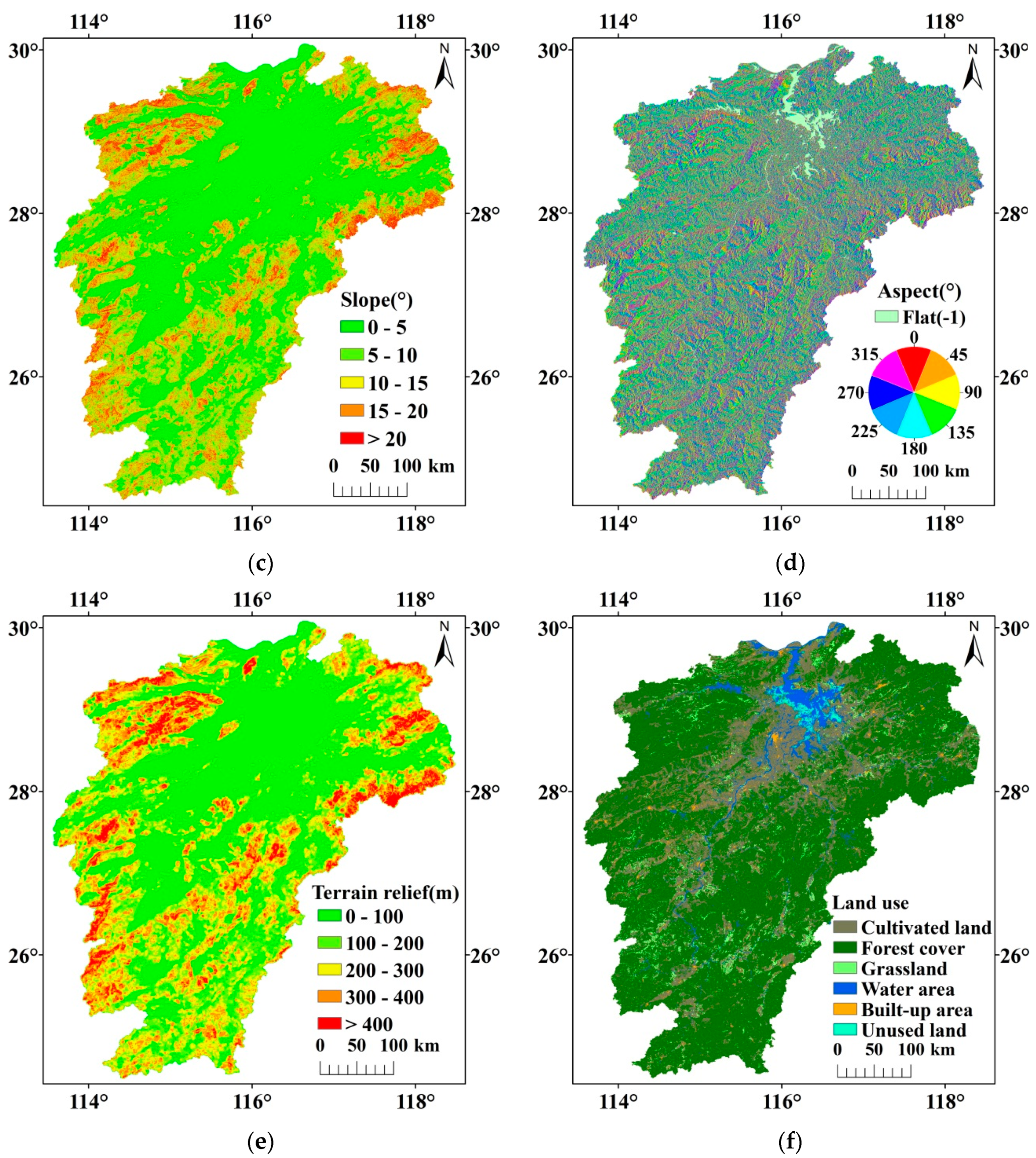
Many experiments indicated that terrain factors and land use have a great impact on SRTM DEM errors [8,17,23]. Thus, they should be considered for the enhancement of SRTM DEM. Here, terrain factors including DEM elevation (Figure 1b), slope (Figure 1c), aspect (Figure 1d) and terrain relief (Figure 1e) were extracted from the SRTM3 DEM. Here, terrain relief is the maximum elevation minus minimum elevation in the 21 × 21 kernel. The selection of the kernel size is based on the conclusion of Lang et al. [41]. In the paper, they first computed the terrain reliefs under different kernel sizes, and then the terrain reliefs with respect to kernel sizes were fitted with a curve. It is found that the curve has an obvious inflection point between the kernel sizes of 19 × 19 and 21 × 21, and becomes flat when the kernel size exceeds 21 × 21. Thus, it is regarded that the kernel size of 21 × 21 is more suited for the extraction of terrain reliefs.
To evaluate the influence of terrain elevation, slope and relief on SRTM3 DEM errors, the reliefs and elevations were evenly grouped into five classes: 0–100, 100–200, 200–300, 300–400, and >400 m, and the slopes were classified into five classes: 0–5, 5–10, 10–15, 15–20 and >20°.
The 30-m land use map (Figure 1f) in the study site was produced by Chinese Academy of Sciences in 2000, with an overall classification accuracy of 92.7% [42]. It includes six classes: cultivated land (27.1%), forestland (62.2%), grassland (4.4%), water area (4.1%), built-up land (1.7%), and unused land (0.5%). Here, unused land is a type of land use that is covered by barren sand, Gobi desert, saline soil, marsh or rock.
For the following analysis and computation, the three terrain factors, land use and the elevation of SRTM3 DEM were extracted for each ICESat/GLAS point based on the bilinear interpolation in ArcGIS 10.6, since the ICESat/GLAS footprint centroids may not locate on the corresponding pixel centers of the gridded surfaces.

3. Methods

3.1. Processing of ICESat/GLAS Data

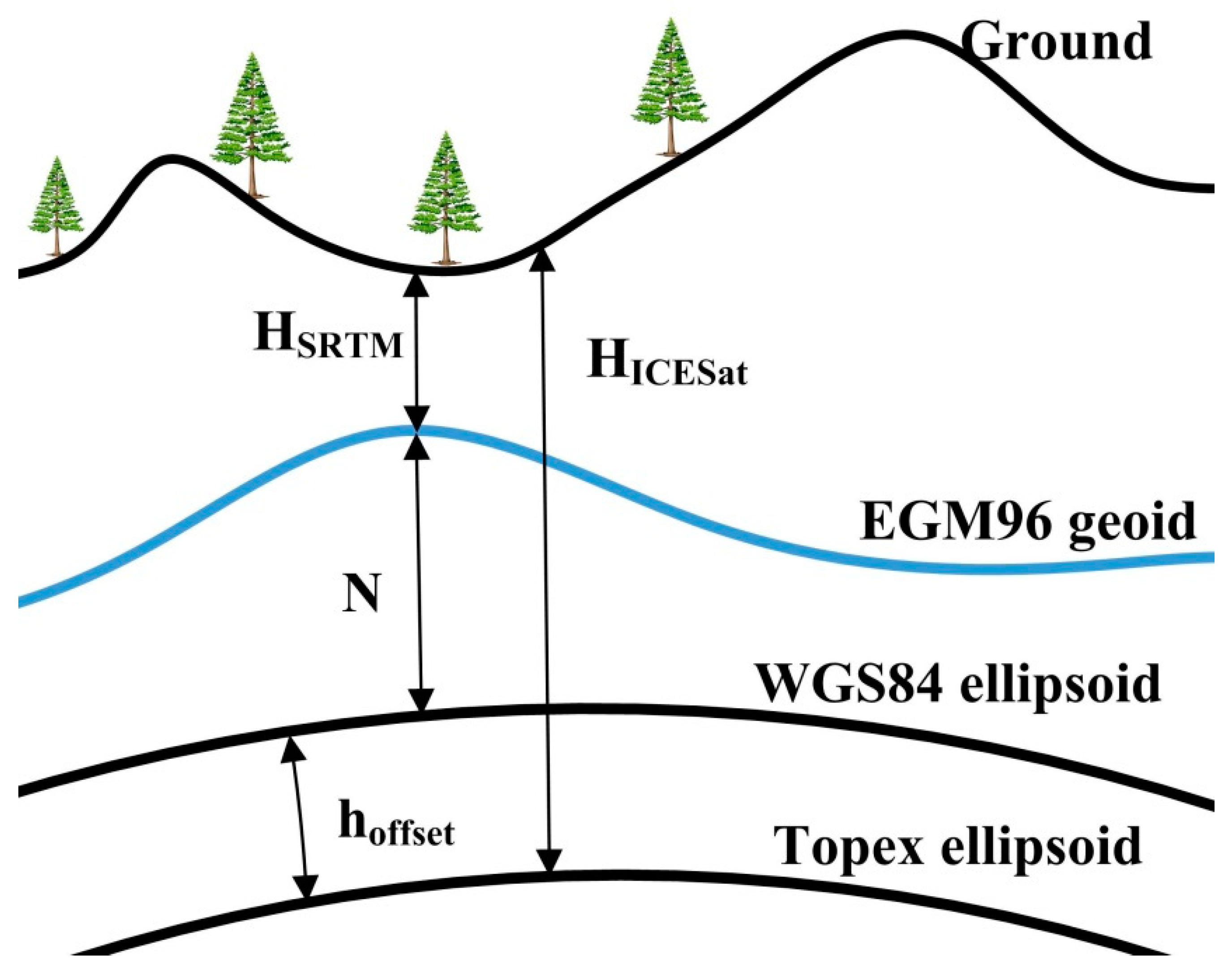
ICESat/GLAS data and SRTM DEM must be homogenized, since the two datasets have different vertical datum. The vertical datum conversion for ICESat/GLAS data from the ellipsoidal height (HICESat) to the orthometric height of SRTM DEM (HSRTM) was achieved by the equation (Figure 2):
H SRTM = H ICESat N h offset
where N is the geoid undulation and hoffset is the vertical datum difference between the TOPEX and the WGS84 ellipsoids, which is a constant. Here, hoffset = 0.707 m [43]. For each ICESat/GLAS elevation, the value of N in Equation (1) was contained in the product referred to as GLAH14 [44].
To assure the accuracy of the selected ICESat/GLAS data, we adopted the following criteria as recommended by some studies [31,32,45]: signal width less than 25 m, peak number less than 6 and received energy lower than 10 FJ. Namely, ICESat/GLAS points which meet the aforementioned conditions were selected for subsequent operations. Outliers commonly exist in ICESat/GLAS data because of the impact of saturated waveforms [46], cloud and valley fog. Thus, elevation differences (EDs) between ICESat/GLAS points and the corresponding SRTM3 DEM values larger than 100 m were removed, as suggested by Carabajal and Harding [47]. Finally, in terms of ED, the ICESat/GLAS points beyond the three standard deviations of the mean were further removed based on the 3-sigma rule [48]. After above steps, 175,684 ICESat/GLAS points were left over the study site.
For the GNSS-based check points, we transformed their elevations (Hcontrol) from Huang-Hai Elevation System 1956 to that of SRTM DEM using the equation:
HSRTM = Hcontrolhoffset
where hoffset is the vertical offset between the two Elevation Systems. Here, Hoffset = 0.357 m [49].

3.2. Coregistration of 3-Arc-Second Shuttle Radar Topography Mission (SRTM3) DEM and ICESat/GLAS Data

As discussed above, the horizontal shift has an effect on the accuracy assessment of DEMs, especially in steep slope areas. Thus, the 3CM, proposed by Nuth and Kääb [50], was employed to eliminate the offset between ICESat/GLAS data and SRTM3 DEM. Data coregistration is based on the following equation:
Δ h / tan ( s ) = x 1 · cos ( x 2 φ ) + x 3
where ∆h is the elevation difference between the ICESat/GLAS point and the corresponding SRTM3 DEM value; s and φ represent terrain slope and aspect, respectively; xi, i = 1, 2, 3 respectively stand for horizontal shift magnitude, shift vector direction and mean bias ( Δ h ¯ ) divided by the tangent of mean slope ( s ¯ ), i.e., x 3 = Δ h ¯ / tan ( s ¯ ) .
Equation (3) shows that the inputs of 3CM include elevation differences between ICESat/GLAS points and the corresponding SRTM3 DEM pixels, terrain slopes and aspects. By solving Equation (3) with a nonlinear least squares fitting method (e.g., Levenberg–Marquardt), the parameters xi, i = 1, 2, 3 can be estimated. Thus, the mean horizontal shifts along the x and y directions (∆x and ∆y) are computed respectively as
x = x1·sin(x2)
y = x1·cos(x2)
Moreover, the mean elevation bias is estimated as
Δ h ¯ = x 3 · tan ( s ¯ )
Based on above results, SRTM3 DEM is co-registered to ICESat/GLAS points by respectively shifting SRTM3 DEM in the x and y directions with the magnitudes of ∆x and ∆y, and then in the vertical direction with the magnitude of Δ h ¯ .
It can be concluded that 3CM has the following merits: (i) simplicity since it does not require other specialized software; (ii) robustness since it considers not only elevation differences between the two datasets, but also terrain parameters; (iii) universality since it can handle any two elevation datasets without the restriction of data collection sensors; and (iv) automation since it does not require manual intervention.

3.3. SRTM3 DEM Correction

To improve the quality of SRTM3 DEM using ICESat/GLAS data, the relationship between ICESat/GLAS elevations (HICESat), terrain factors and land uses was respectively simulated using MLR, RF, BPNN, and GRNN, and their results were compared and analyzed. The general relationship is expressed as
H ICESat = f ( L a t , L o n , H SRTM , S l , R e , A s , L u )
where f(•) is a mapping function, quantitatively shows the relationship between dependent variable and its covariates; Lat and Lon represent latitude and longitude, respectively; Sl, Re, and As are slope, relief and aspect, respectively; Lu is the land-use type and HSRTM is the elevation of SRTM3 DEM at the ICESat/GLAS point.
Since aspect degree is a direction, we used the sine and cosine values of the aspect in the model. Because land-use type is considered as categorical variable [51], five dummy variables were included in the model to represent the six land-use types. More specifically, taking the cultivated land (CL) as the reference, the other five land-use types including forestland (FL), grassland (GL), built-up land (BL), water area (WA), and unused land (UL) were used as dummy variables in the model. This indicates that the land-use type of a point can be described with five dummy variables. For example, if a point has the land-use type of forestland, it can be described as FL = 1 and other four dummy variables are 0 (i.e., GL = 0, BL = 0, WA = 0, and UL = 0). In comparison, if all five dummy variables are 0, the point has the land-use type of cultivated land.

3.3.1. Multiple Linear Regression (MLR)

The formulation of MLR is expressed as
H ICESat = β 0 + i = 1 n β i · x i
where βi (i = 0, … n) are the unknown coefficients to be computed and x = [ x 1 x n ] represent the predictors of SRTM DEM accuracy, as shown in Equation (7). Generally, the linear model is effective to explain the linear relationship [51,52], yet has a poor performance for dealing with nonlinear problems.
In our study, MLR was conducted in Statistical Package for the Social Sciences (SPSS) 22.0.

3.3.2. Back Propagation Neural Network (BPNN)

BPNN is one of the most popular ANNs for solving nonlinear problems. It generally includes three layers (Figure 3): one input layer, one hidden layer and one output layer. Each layer has some neurons: the neuron numbers in the input and output layers equal to the input and output parameters, respectively. According to previous studies [53], the neuron number in the hidden layer ranges from 2 a + b to 2a + 1, where a and b are the neuron number in the input and output layers, respectively. In our study, based on the 10-fold cross valuation scheme [54], the neuron number in the hidden layer was set to 2a + 1, and the transfer functions for the hidden and output layers was set to ‘tansig’ and ‘purelin’, respectively. Moreover, the network consists of connections between the layers and each connection is assigned a weight that represents its relative importance. The BP algorithm was employed to train the multilayer networks for updating weights to minimize the loss function.
In the study, BPNN was conducted in MATLAB R2019b using the commands of “newff”, “train” and “sim” to create a feed-forward backpropagation network, train the network and simulate the network for a new input, respectively.

3.3.3. Generalized Regression Neural Network (GRNN)

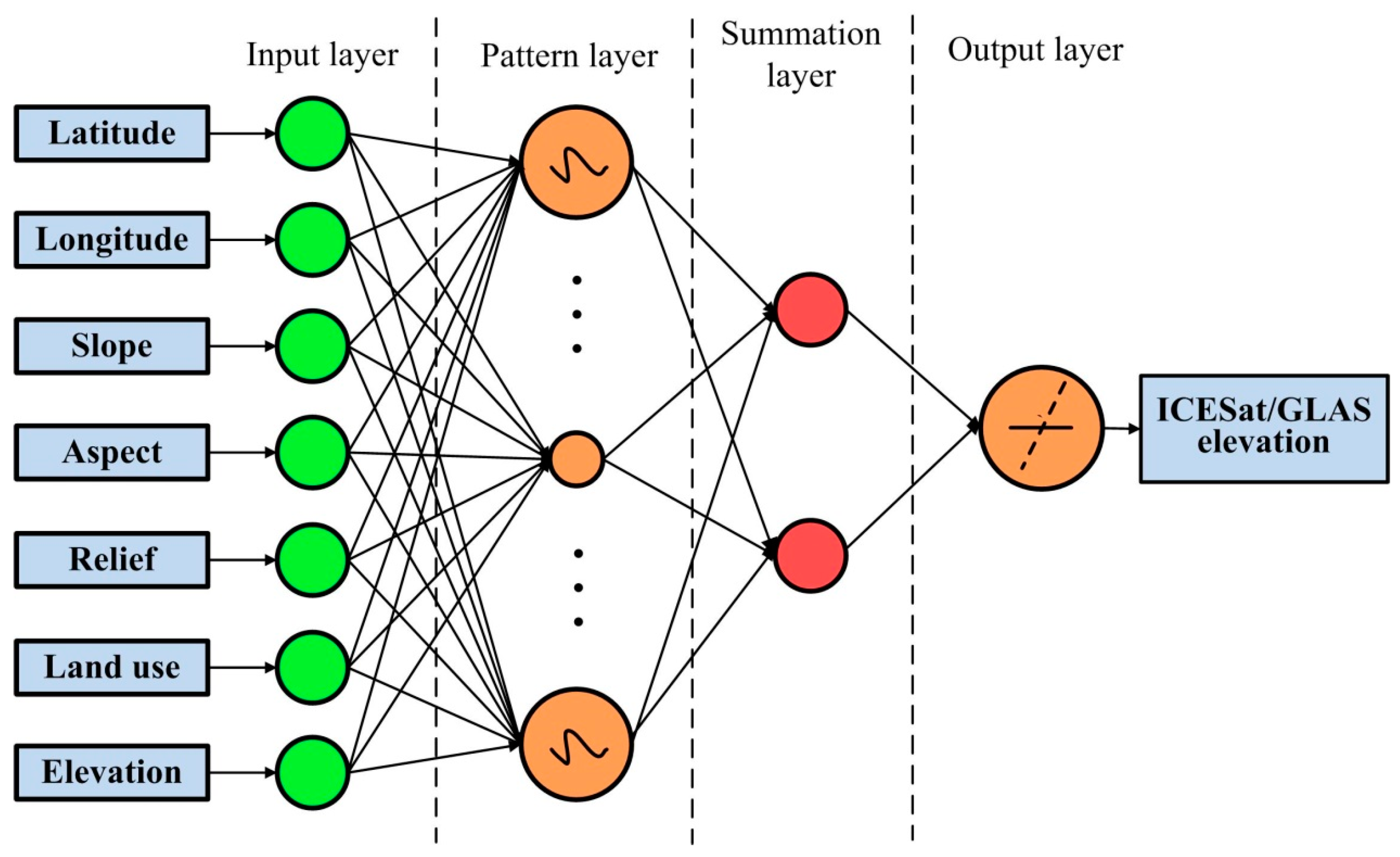
A GRNN includes four layers (Figure 4): input layer, pattern layer, summation layer and output layer. GRNN has the merit of highly computational speed [55], since its weights are pre-determined with a Gaussian function.
The output of GRNN can be formulated as
f ( x ) = i = 1 n z i exp ( d i 2 2 λ 2 ) i = 1 n exp ( d i 2 2 λ 2 )
where n is the number of training samples, zi is the output of the ith training sample, di is the Euclidean distance between the point x to be estimated and the ith training point xi, i.e., d i = x x i 2 and λ is the smoothing parameter of GRNN.
Generally, the larger the value of the smoothing parameter λ, the smoother the function approximation will be. On the contrary, to fit data closely, a smaller value of λ should be used. Thus, the value of the smoothing parameter controls the performance of GRNN. Here, the optimal value of λ was tuned by the 10-fold cross validation.
In our study, GRNN was conducted in MATLAB R2019b using the commands of “newgrnn” and “sim” to design a network and simulate the network for a new input, respectively.

3.3.4. Random Forest (RF)

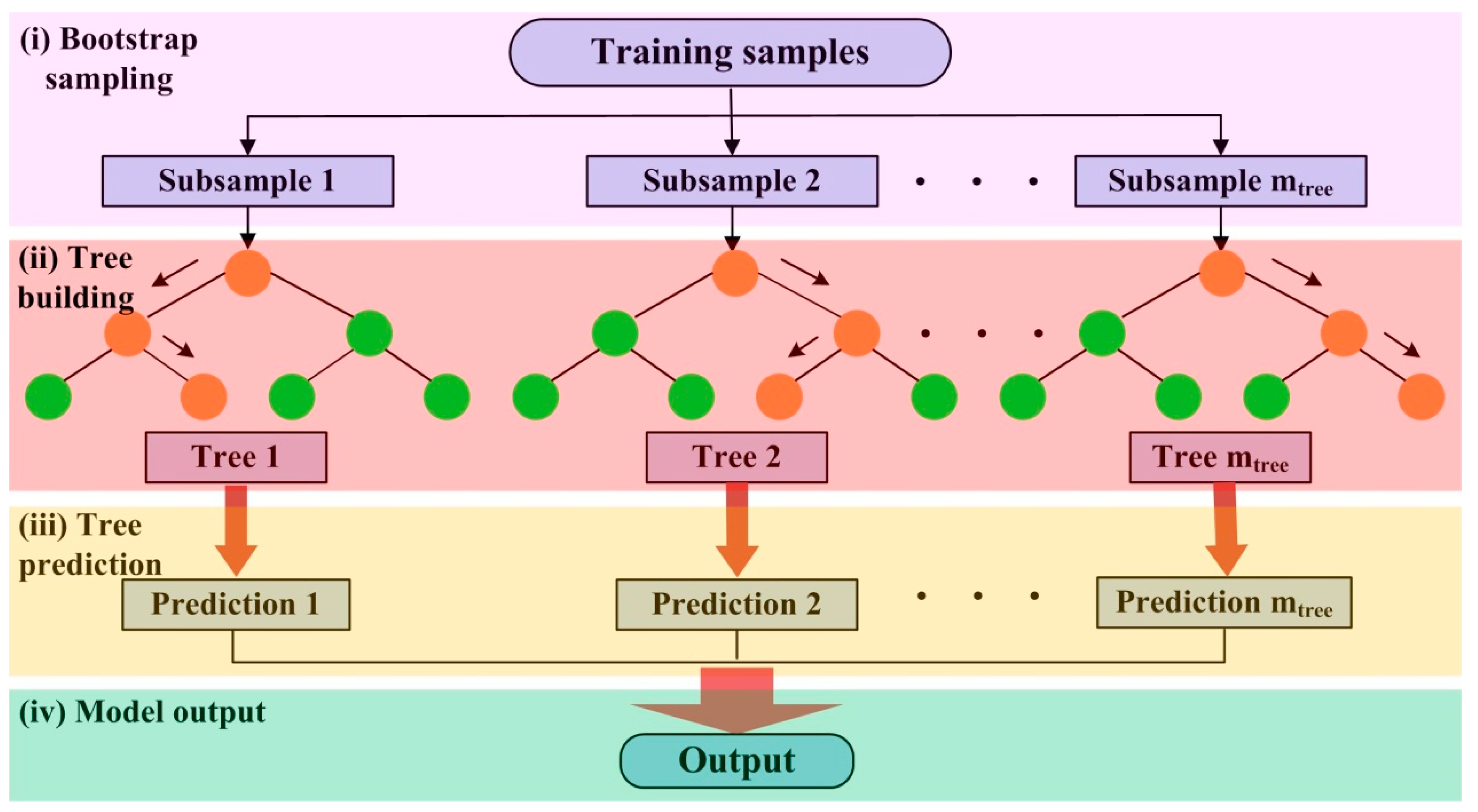
The RF model developed by Breiman [56] is an ensemble learning algorithm based on decision trees and bagging [57,58]. As shown in Figure 5, RF includes four stages: (i) selecting mtree subsamples from the original training samples using bootstrapping; (ii) building mtree independent decision trees with ncov covariates randomly chosen from all independent variables; (iii) performing prediction using each decision tree; and (iv) obtaining the final output by averaging the mtree predictions for regression or taking a simple majority vote for classification [59].
It can be found that RF includes two parameters, i.e., the number of trees (mtree) in the forest and the number of covariates (ncov) in the random subsample. The bootstrapping method and the random selection of the subset of covariates reduces the redundancy of explanatory variables, thereby avoiding the overfitting problem [60]. Additionally, RF has the merits of simplicity, flexibility, ease of use, efficiency, stable computation and automatic rank of feature importance on the prediction, all of which make the method appealing for handling nonlinear problems.
In our test, the RF regression model was performed with the freely available codes, downloaded from the website (https://code.google.com/archive/p/randomforest-matlab/downloads), and the optimal values of the two parameters were determined by the 10-fold cross validation.

3.4. Accuracy Measures

Both root mean square error (RMSE) and mean error (ME) [61] were taken as the accuracy measure to assess the accuracy of SRTM3 DEM and the performance of the DEM correction models. RMSE and ME are formulated respectively as
RMSE = i = 1 n ( O i S i ) 2 n
ME = i = 1 n ( O i S i ) n
where n is the number of check points. For accuracy assessment, Oi and Si respectively represent the elevations of the ith ICESat/GLAS point and the corresponding SRTM3 DEM pixel. For evaluating the performance of DEM correction model, ICESat/GLAS points were randomly grouped into training and testing points with the proportions of 90% and 10%, respectively. More specifically, the former was first adopted to train the model and then the SRTM3 DEM was improved with the trained model. Finally, the testing points were employed to assess the accuracy of the enhanced SRTM3 DEM. Thus, O and S respectively represent the sampled elevations and the corresponding values of the enhanced SRTM3 DEM.
It is undoubtable that more check points can make the accuracy assessment and enhancement more reliable. Moreover, all ICESat/GLAS points can be easily downloaded from the website. Thus, from the point view of the rationality and practicability, all available ICESat/GLAS data were used for assessing and enhancing SRTM3 DEM in our study.
As described in previous Sections, the parameters of each machine learning method were tuned by the 10-fold cross validation in our study. More specifically, given one set of parameters, the 10-fold cross validation was performed as follows [54,62]: (i) averagely dividing the training points into 10 subsamples, and setting the counter variable i = 1, (ii) using the ith subsample for model validation and the other subsamples for model training, (iii) doing i = i + 1, (iv) repeating (ii)–(iii) until i > 10, (v) computing the accuracy measures like RMSE and ME. After several tests, the best parameter values correspond to the least RMSE or ME.

4. Results and Discussion

4.1. Overall Accuracy

Results indicate that based on data coregistration, the mean horizontal shifts of the SRTM3 DEM in the x and y directions with respect to ICESat/GLAS data are −17.588 m (move left) and −29.343 m (move down), respectively. In other words, the SRTM3 DEM relative to ICESat/GLAS data has a subpixel misregistration. In addition, the mean vertical shift of the SRTM3 DEM relative to ICESat/GLAS data is −2.107 m, demonstrating that it is averagely above ICESat/GLAS data. In fact, the horizontal shift between SRTM3 DEM and other DEMs or GCPs was also found in previous studies. For example, Rexer and Hirt [63] revealed an average −0.007 arc-seconds offset in North–South direction and −0.100 arc-seconds offset in East–West direction between ASTER GDEM and SRTM3 DEM over the Australian continent. Satgé et al. [23] found that compared to ICESat/GLAS points, SRTM3 DEM V4.1 has 3.7 and −7.3 m horizontal shifts in the NE–SW and NW–SE directions over the Altiplano watershed, respectively. Li et al. [64] indicated that the horizontal shifts between SRTM3 and ASTER DEMs at three sites of China range from 12.2 to 15.5 m and from 1.4 to 14 m in the x- and y-directions, respectively.
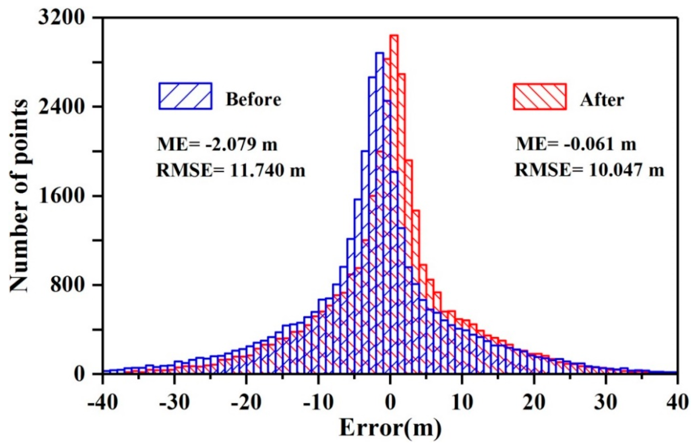
Figure 6 shows that before data coregistration, SRTM3 DEM has a negative bias with the ME of −2.079 m, exhibiting that the SRTM3 DEM is averagely higher than the ICESat/GLAS points. This result is expected as SRTM radar center is located somewhere between vegetation canopy and the bare-earth ground [11,28,47]. The computed RMSE of 11.740 m is within the specified accuracy of the SRTM DEM (i.e., 16 m). The RMSE in this study is approximate to the values in South America and other regions of China. For example, Huang et al. [29] showed that the SRTM3 DEM over the eastern Tibetan Plateau of China has the RMSE of 15.2 m. Du et al. [30] found that the RMSE of SRTM3 DEM over Pearl River Delta area of China is 14.01 m. Satgé et al. [23] reported that the RMSE of SRTM3 DEM over the Altiplano watershed is 11.1 m.
After the coregistration, the DEM vertical errors are symmetrically distributed around zero with the ME of −0.061 m, while the RMSE is 10.047 m. This indicates that data misregistration significantly affects the vertical accuracy of SRTM3 DEM. Specifically, after the data coregistration, the ME and RMSE of SRTM3 DEM are decreased by 97.1% and 14.4%, respectively. However, this data preprocess was commonly omitted in previous researches [32,43,44,65], which may result in a large RMSE. For example, without the coregistration, Zhao et al. [44] demonstrated that the SRTM3 DEM relative to ICESat/GLAS data over the Shanbei Plateau, China has the RMSE of 20.72 m and the ME of −1.0 m.

4.2. Effect of Terrain Factors and Land Use on SRTM3 DEM Errors Relative to ICESat/GLAS Data

4.2.1. Terrain Factors

Figure 7a shows that without data coregistration, SRTM3 DEM errors with a sine-like shape are strongly associated with terrain aspects. This indicates the misalignment of SRTM3 DEM and ICESat/GLAS data, since a strong relationship between terrain aspects and DEM errors is a useful indicator of data misregistration [33]. Although this relationship was also found by some researchers [8,17,44], there is no doubt about its cause from data misalignment or inaccurate alignment. With the coregistration, this relationship seems to disappear (Figure 7b). Therefore, without the coregistration, terrain aspect might be wrongly taken as a dominant explanatory factor for SRTM3 DEM errors. Figure 7b shows that SRTM3 DEM obtains the lowest accuracy in the north direction (i.e., aspect values are around 0° and 360°), and the highest accuracy in the south direction (i.e., aspect values are around 180°). This is attributed to the fact that for collecting elevation data using SAR technique, the data on the foreslopes (facing the sensor) have a high accuracy, while those on the backslopes are much poorly measured, especially in steep slope areas [66].
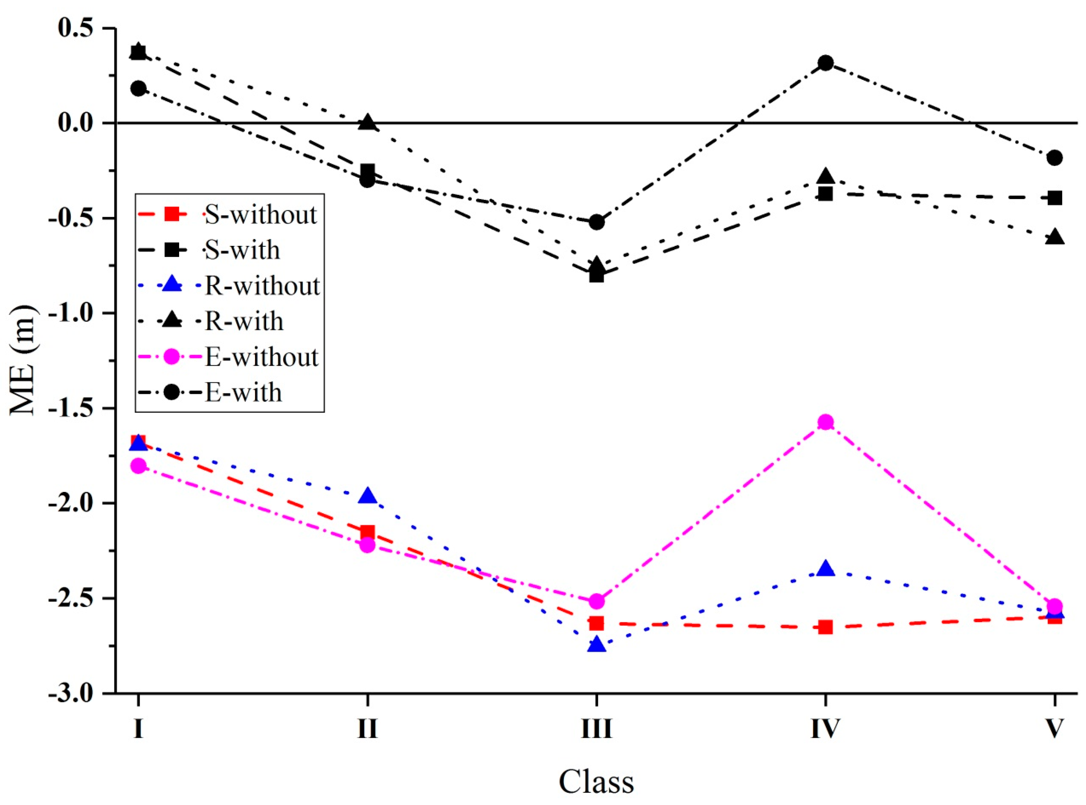
Table 1 and Figure 8 demonstrate the influence of terrain slope, relief and elevation classes on the MEs of SRTM3 DEM without and with data coregistration. It is obvious that no relationship is found between the ME and the three terrain factors on all classes, mainly because of the different penetration ability of SRTM radar signal under different environments. For all the classes without data coregistration, the MEs are about −2 m. After the coregistration, the systematic biases are significantly reduced. Moreover, the MEs on the first class (I) of the three terrain factors, and on the fourth class (IV) of elevation are positive. This is owed to the fact that these classes are mainly covered by water body and flat terrain, which have a smaller bias than the other land uses. In fact, the complex relationship between ME and the terrain slope was also reported by previous studies [17,44,65].
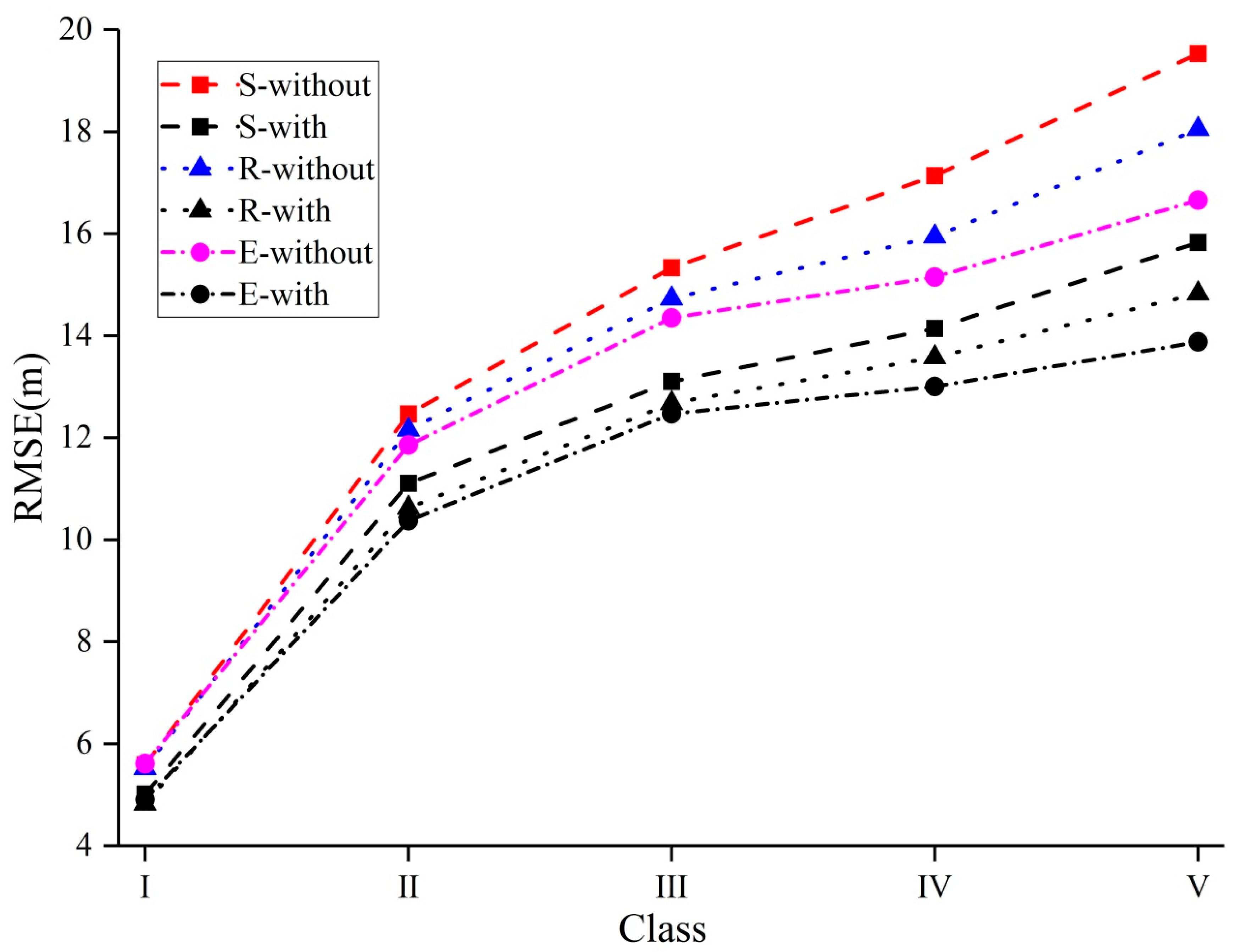
Table 1 and Figure 9 exhibit that for the classes II–V, there exists a strong positive relationship between RMSEs and terrain factors. However, for class I, the RMSEs are obviously smaller than those of the other classes. This is because class I has a flat terrain and SRTM3 DEM has a much higher accuracy in such terrain than in the other terrain types. The RMSEs with data coregistration are consistently smaller than those without the coregistration on all the classes. In comparison, SRTM3 DEM has the largest accuracy improvement on class V, since this class is mainly covered by dense forests, where the SRTM radar signal has the lowest penetration depth.
Our results on the relationship between terrain factors and SRTM3 DEM errors are consistent with previously reported findings. For example, Szabó et al. [67] assessed the accuracy of SRTM3 V2 and V3 in two mountainous areas of Hungary and found that their error standard deviations (STDs) increased from 4.28 and 3.16 m on the slope class 0–5° to 9.8 and 8.02 m on the class >20°, respectively. Satgé et al. [23] demonstrated that the RMSE of SRTM3 DEM V4 over the Altiplano watershed in South America increases from 8.1 to 21.1 m when the slope class ranges from 0–2° to >20°. Zhang et al. [17] indicated that the STD of SRTM3 DEM changes from 4.29 m with the slope class 0–2° to 17.51 m of slope greater than 35° over the whole of China. Plenty of studies demonstrated that in addition to SRTM DEM, the vertical accuracy of other public DEMs also shows a strong negative relationship with terrain slope [19,65,68,69,70].

4.2.2. Land Use

Table 1 and Figure 10 show that land-use type has a great influence on SRTM3 DEM errors. More specifically, without data coregistration, the ME ranges from −0.70 m in water area to −2.55 m in cultivated land (Figure 10a), while the RMSEs from 1.78 m in unused land to 13.84 m in forested cover (Figure 10b). Namely, among the six land uses, forest area has the largest RMSE. This is an expected result, as tree trunks and limbs can cause irregular backscattering of SRTM radar signal, thereby magnifying the geometric distortions [43]. After data coregistration, the accuracy of SRTM3 DEM is significantly improved on almost all land uses, except for the water area. This is because the raw SRTM3 DEM has voids over water bodies, which were filled by other datasets in the production of SRTM3 DEM V4.1 [71]. Obviously, the data used for void filling has a low systematic bias (i.e., −0.70 m). Thus, the fact that the biases in the slope class of 0–5°, elevation and terrain relief classes of 0–100 m become positive after the coregistration (Figure 8) is mainly due to the large proportion of water bodies in the three classes.
The poor performance of global DEMs in forested areas was also reported in other studies. For example, Hu et al. [72] assessed the accuracy of different public DEMs of Hubei province, China, and indicated that compared to built-up areas, wetland and cultivated land areas, forest area produces the lowest accuracy. Li and Zhao [65] evaluated the errors of AW3D30 in function of land cover, and obtained that the forest gives the poorest accuracy, which is followed by grassland. Yap et al. [20] evaluated freely available latest 30-m DEMs over Cameroon and pointed out that all DEMs have the worst performance in the areas characterized by forests and shrubs. From our test and the previously reported results, it can be concluded that the forest areas have the poorest accuracy mainly due to the low penetration and irregular backscattering of SRTM radar signals.

4.3. Model Performance Comparison

Table 2 shows the performance of MLR and the three machine learning methods for the correction of SRTM3 DEM with and without data coregistration. Note that the automated 3D data coregistration method (3CM) introduced in this paper can be also considered as a correction method, since after the coregistration, the DEM accuracy is improved. Thus, its performance is compared with those of the other correction models.
It can be found that without data coregistration, MLR, BPNN, GRNN and RF have lower MEs and RMSEs than those of the original SRTM3 DEM (ME = −2.079 m and RMSE = 11.740 m). Namely, the four models improve the accuracy of the original SRTM3 DEM. However, in terms of ME, only MLR (ME = −0.045 m) and BPNN (ME = −0.029 m) outperform 3CM (ME = −0.061 m), while in terms of RMSE, only BPNN (RMSE = 9.793 m) yielded a better result than 3CM (RMSE = 10.047 m). With the data coregistration, almost all models perform better than 3CM, except for GRNN in terms of RMSE. Specifically, in terms of RMSE, MLR, BPNN, and RF are 5.4%, 5.8%, and 8.3% more accurate than 3CM, respectively, while GRNN is 3.2% less accurate than 3CM. The poor performance of GRNN might be attributed to the fact that its weighted computation (i.e., Equation (8)) is too simple to capture the nonlinear relationship between the predictors and SRTM3 DEM errors. The four models with data coregistration significantly outperform themselves without the coregistration. For instance, after data coregistration, the ME and RMSE of GRNN are reduced by 80.8% and 9.4%, respectively. Hence, data coregistration is essential for SRTM3 DEM correction.
In contrast, the four models with the data coregistration produce similar results for the bias elimination of SRTM3 DEM, as their absolute MEs are approximate to 0, especially for BPNN with ME = −0.003 m. With respect to RMSE, RF outperforms the other models. Specifically, RF is about 8.3%, 3.1%, 2.7%, and 11.3% more accurate than 3CM, MLR, BPNN, and GRNN, respectively. The high accuracy of RF is mainly attributed to its ensemble learning technique [56,73]. Moreover, the RF regression employed a bootstrap aggregation scheme to collect some data from all samples to train the model and other to validate the model. This strategy avoids the overfitting problem, which commonly confuses linear regression method and the classical machine learning methods [74].
The computational costs indicate that MLR has the fast speed, which is followed by 3CM. This is expected, as the two methods do not solve large linear systems. Among the three machine learning methods, RF has the largest computing cost, since it includes four stages, each of which is time-consuming.
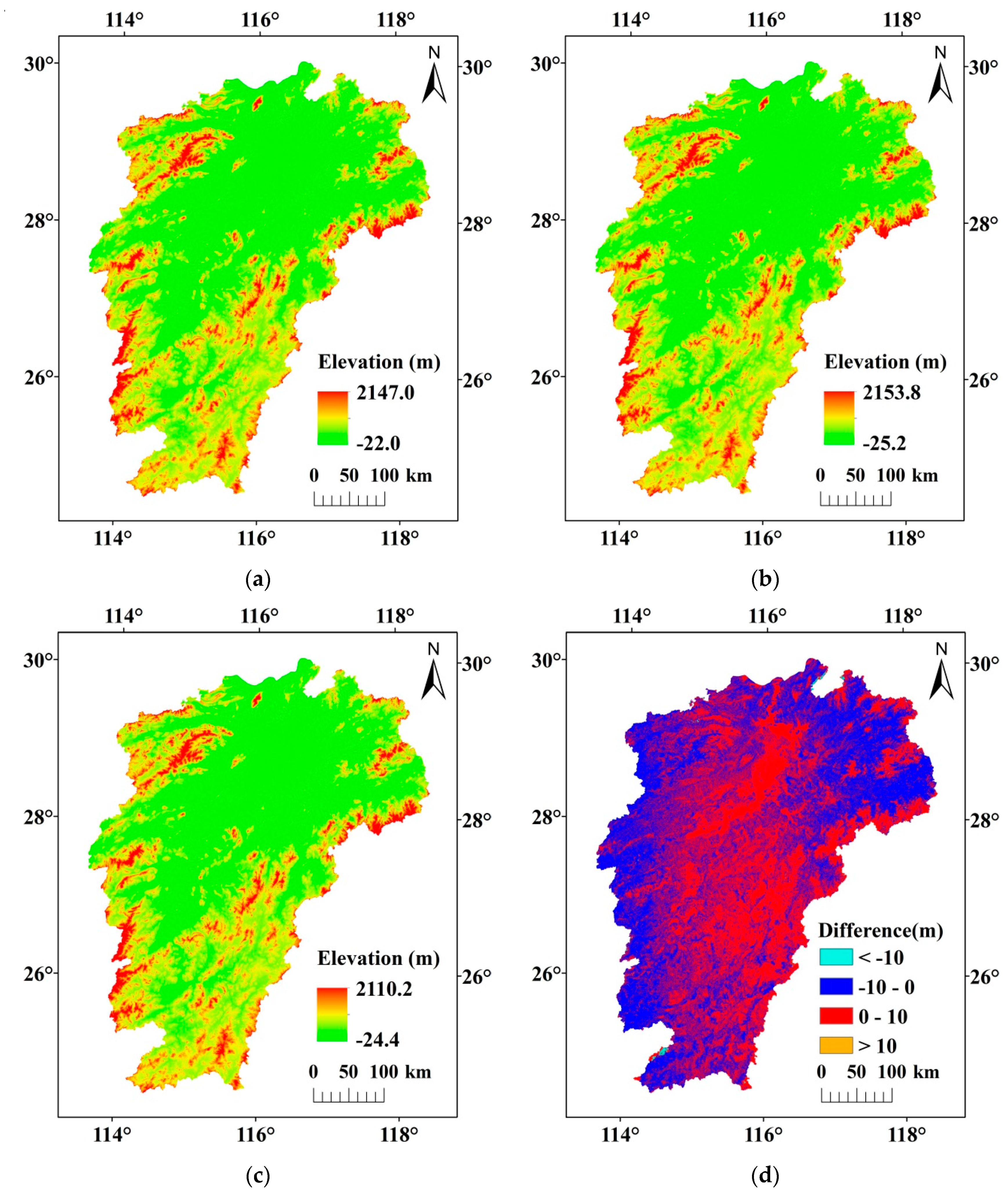
Additionally, the corrected DEMs based on MLR and RF are compared, since the two models are representative of linear and nonlinear regressions, respectively. Figure 11 shows that the corrected DEMs based on MLR (Figure 11b) and RF (Figure 11c) have a similar appearance to the original one (Figure 11a). However, the high elevations of the two corrected DEMs (i.e., points with red color) are obviously less than those of the original DEM. This is expected as the elevations of the points located in forested areas are accurately corrected by the models. It is surprised to see that the maximum value of MLR-based DEM (i.e., 2153.8 m) is slightly larger than that of the original one (i.e., 2147.0 m). This seems unreasonable, as the highest point is more likely located on mountain, which is covered by forests, and these points should be lowered. In comparison, RF clearly lowers the highest elevation, indicating that the negative effect of the forest canopy on SRTM3 DEM was reduced. The difference between the RF-based and MLR-based DEMs (Figure 11d) shows that the elevations of RF in the forest areas are lower than those of MLR. This further indicates that RF is more effective than MLR for enhancing SRTM3 DEM, especially in forest areas.
Finally, the GNSS-derived check points were employed to assess the accuracy of the RF-enhanced DEMs with and without data coregistration. Results (Table 3) show that the enhanced SRTM3 DEM with data coregistration is more accurate than that without the coregistration. Specifically, compared to the ME and RMSE without the coregistration, those with the coregistration are reduced by 74.5% and 8.2%, respectively. Moreover, the enhanced DEM accuracy relative to the GNSS points is slightly lower than that relative to the ICESat/GLASS data. This might be owed to the different locations of the two groups of the check points. Specifically, the GNSS points are located in Ganzhou city, while the ICESat/GLAS data are located in Jiangxi province. However, the local accuracy assessment is helpful for our understanding of the quality of the enhanced SRTM3 DEM. Therefore, it can be concluded that the accuracy of the enhanced DEM is improved by the RF method.
In previous works, the ICESat/GLAS-based correction of SRTM DEM was conducted under different areas. For example, Satgé et al. [23] improved SRTM3 DEM by removing its bias from ICESat/GLAS points over the Altiplano watershed in South America. Compared to the original SRTM3 DEM, the RMSE of the enhanced one was reduced by 22.5%. Zhao et al. [44] employed MLR to improve the SRTM3 DEM based on ICESAT/GLAS data over the Shanbei Plateau, China, where the RMSE was reduced by 54.4%. Wendleder et al. [38] used spherical harmonics to remove the error of SRTM3 DEM based on ICESat/GLAS data at a global scale, and found that the mean error was reduced by 66.7%. Similarly, Yue et al. [32] employed ANNs to improve the accuracy of ASTER GDEM with ICESat/GLAS data on a global scale. Therefore, the ICESat/GLAS-based correction of SRTM DEM can be achieved at different scales including regional-, watershed- and global-scales. It is obvious that their accuracy improvement levels are inconsistent. This is because the accuracy of the improved SRTM3 DEM seriously depends on terrain characteristics, land uses, forest types, and model performance.

5. Conclusions

Data coregistration between SRTM DEM and ICESat/GLAS data were commonly omitted in the context of DEM accuracy assessment and correction in previous researches. In this paper, a simple and general 3D data coregistration method (3CM) is introduced and used to co-register the two datasets, and then its influence on the accuracy of SRTM DEM is analyzed. Results show that the 3-arc-second SRTM (SRTM3) DEM has a subpixel misregistration relative to ICESat/GLAS data, with the mean horizontal shifts in the x- and y-directions of −17.588 and −29.343 m, respectively. Moreover, the vertical shift is −2.107 m. After data coregistration, the mean bias and RMSE of SRTM3 DEM are −0.061 and 10.047 m, respectively, which are less than those without the coregistration. The effect of terrain factors including aspect, slope, elevation and relief, and land use types on the vertical accuracy of SRTM3 DEM is analyzed. The results demonstrate that there is a strong relationship between aspect and SRTM3 DEM errors before data coregistration; however, this relationship disappears after data coregistration. The vertical bias of SRTM3 DEM has no conclusive relationship with the three terrain factors, while the DEM RMSE linearly increases with the increase of terrain factors. Data coregistration greatly improves the accuracy of SRTM3 DEM on almost all the classes of the terrain factors. Among the six land use types, the forest areas produce the largest vertical errors.
The terrain factors and land uses were incorporated into the models including MLR, BPNN, GRNN, and RF for the correction of SRTM3 DEM. It is found that without data coregistration, the 3CM seems more accurate than the four models. However, after the coregistration, the performances of the four models are greatly improved. Among the four models, the RF method produces the best result, which is about 3.1%, 2.7%, and 11.3% more accurate than MLR, BPNN, and GRNN in terms of RMSE, respectively. However, it has the largest computational cost. Accuracy assessment of the RF-enhanced SRTM3 DEM relative to 146 GNSS points located in Ganzhou city also shows its quality improvement. Overall, our results clearly demonstrate the importance of data coregistration for accuracy assessment and enhancement of SRTM3 DEM using ICESat/GLAS data. Since all of the methods used in this paper are simple, general, and effective, they could be applied to other publicly available DEMs, such as ASTER GDEM, Advanced Land Observing Satellite (ALOS) World 3 Dimensions (3D) 30 m (AW3D) DEM, and TerraSAR-X add-on for Digital Elevation Measurements (TanDEM-X) DEM in the context of accuracy assessment and enhancement.

Author Contributions

Conceptualization, methodology, and writing, C.C.; data curation, investigation, and visualization, S.Y., methodology, Y.L. All authors have read and agreed to the published version of the manuscript.

Funding

This work was supported by the National Natural Science Foundation of China (Grant No. 41371367, 41804001), Shandong Provincial Natural Science Foundation, China (Grant No. ZR2019MD007, ZR2019BD006), A Project of Shandong Province Higher Educational Youth Innovation Science and Technology Program (Grant No. 2019KJH007), Shandong Provincial Key Research and Development Program (Major Scientific and Technological Innovation Project) (Grant No. 2019JZZY010429) and by the Scientific Research Foundation of Shandong University of Science and Technology for Recruited Talents (Grant No. 2019RCJJ003).

Conflicts of Interest

The authors declare no conflict of interest.

References

  1. Shi, W.; Deng, S.; Xu, W. Extraction of multi-scale landslide morphological features based on local Gi* using airborne LiDAR-derived DEM. Geomorphology 2018, 303, 229–242. [Google Scholar] [CrossRef]
  2. Khosravipour, A.; Skidmore, A.K.; Wang, T.; Isenburg, M.; Khoshelham, K. Effect of slope on treetop detection using a LiDAR Canopy Height Model. ISPRS J. Photogramm. Remote Sens. 2015, 104, 44–52. [Google Scholar] [CrossRef]
  3. Yamazaki, D.; Baugh, C.A.; Bates, P.D.; Kanae, S.; Alsdorf, D.E.; Oki, T. Adjustment of a spaceborne DEM for use in floodplain hydrodynamic modeling. J. Hydrol. 2012, 436–437, 81–91. [Google Scholar] [CrossRef]
  4. Razak, K.A.; Santangelo, M.; Van Westen, C.J.; Straatsma, M.W.; de Jong, S.M. Generating an optimal DTM from airborne laser scanning data for landslide mapping in a tropical forest environment. Geomorphology 2013, 190, 112–125. [Google Scholar] [CrossRef]
  5. Chen, C.; Li, Y. A fast global interpolation method for digital terrain model generation from large LiDAR-derived data. Remote Sens. 2019, 11, 1324. [Google Scholar] [CrossRef] [Green Version]
  6. Wilson, J.P. Digital terrain modeling. Geomorphology 2012, 137, 107–121. [Google Scholar] [CrossRef]
  7. Farr, T.G.; Rosen, P.A.; Caro, E.; Crippen, R.; Duren, R.; Hensley, S.; Kobrick, M.; Paller, M.; Rodriguez, E.; Roth, L. The shuttle radar topography mission. Rev. Geophys. 2007, 45, RG2004. [Google Scholar] [CrossRef] [Green Version]
  8. Shortridge, A.; Messina, J. Spatial structure and landscape associations of SRTM error. Remote Sens. Environ. 2011, 115, 1576–1587. [Google Scholar] [CrossRef]
  9. Rodriguez, E.; Morris, C.S.; Belz, J.E. A global assessment of the SRTM performance. Photogramm. Eng. Remote Sens. 2006, 72, 249–260. [Google Scholar] [CrossRef] [Green Version]
  10. Yamazaki, D.; Ikeshima, D.; Tawatari, R.; Yamaguchi, T.; O’Loughlin, F.; Neal, J.C.; Sampson, C.C.; Kanae, S.; Bates, P.D. A high-accuracy map of global terrain elevations. Geophys. Res. Lett. 2017, 44, 5844–5853. [Google Scholar] [CrossRef] [Green Version]
  11. Su, Y.; Guo, Q. A practical method for SRTM DEM correction over vegetated mountain areas. ISPRS J. Photogramm. Remote Sens. 2014, 87, 216–228. [Google Scholar] [CrossRef]
  12. Hancock, G.R.; Martinez, C.; Evans, K.G.; Moliere, D.R. A comparison of SRTM and high-resolution digital elevation models and their use in catchment geomorphology and hydrology: Australian examples. Earth Surf. Process. Landf. 2006, 31, 1394–1412. [Google Scholar] [CrossRef]
  13. Sharma, A.; Tiwari, K.N. A comparative appraisal of hydrological behavior of SRTM DEM at catchment level. J. Hydrol. 2014, 519, 1394–1404. [Google Scholar] [CrossRef]
  14. Brock, J.; Schratz, P.; Petschko, H.; Muenchow, J.; Micu, M.; Brenning, A. The performance of landslide susceptibility models critically depends on the quality of digital elevations models. Geomat. Nat. Hazards Risk 2020, 11, 1075–1092. [Google Scholar] [CrossRef]
  15. Suwandana, E.; Kawamura, K.; Sakuno, Y.; Kustiyanto, E.; Raharjo, B. Evaluation of ASTER GDEM2 in Comparison with GDEM1, SRTM DEM and Topographic-Map-Derived DEM Using Inundation Area Analysis and RTK-dGPS Data. Remote Sens. 2012, 4, 2419–2431. [Google Scholar] [CrossRef] [Green Version]
  16. Mukherjee, S.; Joshi, P.K.; Mukherjee, S.; Ghosh, A.; Garg, R.D.; Mukhopadhyay, A. Evaluation of vertical accuracy of open source Digital Elevation Model (DEM). Int. J. Appl. Earth Obs. Geoinf. 2013, 21, 205–217. [Google Scholar] [CrossRef]
  17. Zhang, Q.; Yang, Q.; Wang, C. SRTM error distribution and its associations with landscapes across China. Photogramm. Eng. Remote Sens. 2016, 82, 135–148. [Google Scholar] [CrossRef]
  18. Athmania, D.; Achour, H. External Validation of the ASTER GDEM2, GMTED2010 and CGIAR-CSI- SRTM v4.1 Free Access Digital Elevation Models (DEMs) in Tunisia and Algeria. Remote Sens. 2014, 6, 4600–4620. [Google Scholar] [CrossRef] [Green Version]
  19. Li, P.; Shi, C.; Li, Z.; Muller, J.-P.; Drummond, J.; Li, X.; Li, T.; Li, Y.; Liu, J. Evaluation of ASTER GDEM using GPS benchmarks and SRTM in China. Int. J. Remote Sens. 2013, 34, 1744–1771. [Google Scholar] [CrossRef]
  20. Yap, L.; Kandé, L.H.; Nouayou, R.; Kamguia, J.; Ngouh, N.A.; Makuate, M.B. Vertical accuracy evaluation of freely available latest high-resolution (30 m) global digital elevation models over Cameroon (Central Africa) with GPS/leveling ground control points. Int. J. Digit. Earth 2019, 12, 500–524. [Google Scholar] [CrossRef]
  21. Varga, M.; Bašić, T. Accuracy validation and comparison of global digital elevation models over Croatia. Int. J. Remote Sens. 2015, 36, 170–189. [Google Scholar] [CrossRef]
  22. Li, Y.Y.; Xu, C.J.; Chen, C.F.; Yin, H.; Yi, L.; He, X. Adaptive Denoising Approach for High-Rate GNSS Seismic Waveform Preservation: Application to the 2010 EI Mayor-Cucapah Earthquake and 2012 Brawley Seismic Swarm. IEEE Access 2019, 7, 173166–173184. [Google Scholar] [CrossRef]
  23. Satgé, F.; Bonnet, M.P.; Timouk, F.; Calmant, S.; Pillco, R.; Molina, J.; Lavado-Casimiro, W.; Arsen, A.; Crétaux, J.F.; Garnier, J. Accuracy assessment of SRTM v4 and ASTER GDEM v2 over the Altiplano watershed using ICESat/GLAS data. Int. J. Remote Sens. 2015, 36, 465–488. [Google Scholar] [CrossRef]
  24. Zhao, S.; Wang, L.; Cheng, W.; Liu, H.; He, W. Rectification methods comparison for the ASTER GDEM V2 data using the ICESat/GLA14 data in the Lvliang mountains, China. Environ. Earth Sci. 2015, 74, 6571–6590. [Google Scholar] [CrossRef]
  25. Simard, M.; Neumann, M.; Buckley, S. Validation of the new SRTM digital elevation model (NASADEM) with ICESAT/GLAS over the United States. In Proceedings of the 2016 IEEE International Geoscience and Remote Sensing Symposium (IGARSS), Beijing, China, 10–15 July 2016; pp. 3227–3229. [Google Scholar]
  26. Liu, Z.; Zhu, J.; Fu, H.; Zhou, C.; Zuo, T. Evaluation of the Vertical Accuracy of Open Global DEMs over Steep Terrain Regions Using ICESat Data: A Case Study over Hunan Province, China. Sensors 2020, 20, 4865. [Google Scholar] [CrossRef]
  27. Beaulieu, A.; Clavet, D. Accuracy assessment of Canadian Digital Elevation Data using ICESat. Photogramm. Eng. Remote Sens. 2009, 75, 81–86. [Google Scholar] [CrossRef]
  28. Carabajal, C.C.; Harding, D.J. SRTM C-Band and ICESat Laser Altimetry Elevation Comparisons as a Function of Tree Cover and Relief. Photogramm. Eng. Remote Sens. 2006, 72, 287–298. [Google Scholar] [CrossRef] [Green Version]
  29. Huang, X.; Xie, H.; Liang, T.; Yi, D. Estimating vertical error of SRTM and map-based DEMs using ICESat altimetry data in the eastern Tibetan Plateau. Int. J. Remote Sens. 2011, 32, 5177–5196. [Google Scholar] [CrossRef]
  30. Du, X.; Guo, H.; Fan, X.; Zhu, J.; Yan, Z.; Zhan, Q. Vertical accuracy assessment of freely available digital elevation models over low-lying coastal plains. Int. J. Digit. Earth 2016, 9, 252–271. [Google Scholar] [CrossRef]
  31. Huber, M.; Wessel, B.; Kosmann, D.; Felbier, A.; Schwieger, V.; Habermeyer, M.; Wendleder, A.; Roth, A. Ensuring globally the TanDEM-X height accuracy: Analysis of the reference data sets ICESat, SRTM and KGPS-Tracks. In Proceedings of the 2009 IEEE International Geoscience and Remote Sensing Symposium, Cape Town, South Africa, 12–17 July 2009; pp. II-769–II-772. [Google Scholar]
  32. Yue, L.; Shen, H.; Zhang, L.; Zheng, X.; Zhang, F.; Yuan, Q. High-quality seamless DEM generation blending SRTM-1, ASTER GDEM v2 and ICESat/GLAS observations. ISPRS J. Photogramm. Remote Sens. 2017, 123, 20–34. [Google Scholar] [CrossRef] [Green Version]
  33. Van Niel, T.G.; McVicar, T.R.; Li, L.; Gallant, J.C.; Yang, Q. The impact of misregistration on SRTM and DEM image differences. Remote Sens. Environ. 2008, 112, 2430–2442. [Google Scholar] [CrossRef]
  34. Baugh, C.A.; Bates, P.D.; Schumann, G.; Trigg, M.A. SRTM vegetation removal and hydrodynamic modeling accuracy. Water Resour. Res. 2013, 49, 5276–5289. [Google Scholar] [CrossRef] [Green Version]
  35. Zhao, X.; Su, Y.; Hu, T.; Chen, L.; Gao, S.; Wang, R.; Jin, S.; Guo, Q. A global corrected SRTM DEM product for vegetated areas. Remote Sens. Lett. 2018, 9, 393–402. [Google Scholar] [CrossRef]
  36. O’Loughlin, F.E.; Paiva, R.C.D.; Durand, M.; Alsdorf, D.E.; Bates, P.D. A multi-sensor approach towards a global vegetation corrected SRTM DEM product. Remote Sens. Environ. 2016, 182, 49–59. [Google Scholar] [CrossRef] [Green Version]
  37. Wendi, D.; Liong, S.Y.; Sun, Y. An innovative approach to improve SRTM DEM using multispectral imagery and artificial neural network. J. Adv. Model. Earth Syst. 2016, 8, 691–702. [Google Scholar] [CrossRef] [Green Version]
  38. Wendleder, A.; Felbier, A.; Wessel, B.; Huber, M.; Roth, A. A Method to Estimate Long-Wave Height Errors of SRTM C-Band DEM. IEEE Geosci. Remote Sens. Lett. 2016, 13, 696–700. [Google Scholar] [CrossRef] [Green Version]
  39. Zhan, J.; Shi, N.; He, S.; Lin, Y. Factors and mechanism driving the land-use conversion in Jiangxi Province. J. Geogr. Sci. 2010, 20, 525–539. [Google Scholar] [CrossRef]
  40. Robinson, N.; Regetz, J.; Guralnick, R.P. EarthEnv-DEM90: A nearly-global, void-free, multi-scale smoothed, 90m digital elevation model from fused ASTER and SRTM data. ISPRS J. Photogramm. Remote Sens. 2014, 87, 57–67. [Google Scholar] [CrossRef]
  41. Lang, L.; Cheng, W.; Zhu, Q.; Long, E. A Comparative Analysis of the Multi-criteria DEM Extracted Relief—Taking Fujian Low Mountainous Region as an Example. Geo-Inf. Sci. 2007, 9, 1–6. [Google Scholar]
  42. Liu, J.; Liu, M.; Tian, H.; Zhuang, D.; Zhang, Z.; Zhang, W.; Tang, X.; Deng, X. Spatial and temporal patterns of China’s cropland during 1990–2000: An analysis based on Landsat TM data. Remote Sens. Environ. 2005, 98, 442–456. [Google Scholar] [CrossRef]
  43. Bhang, K.J.; Schwartz, F.W.; Braun, A. Verification of the Vertical Error in C-Band SRTM DEM Using ICESat and Landsat-7, Otter Tail County, MN. IEEE Trans. Geosci. Remote Sens. 2007, 45, 36–44. [Google Scholar] [CrossRef]
  44. Zhao, S.; Zhao, H.; Li, R.; Cheng, W.; Zhou, C. A quantitative model to simulate the vertical errors of SRTM3 DEM V4 data at the pixel level in the Shanbei Plateau of China. Int. J. Remote Sens. 2020, 41, 5257–5276. [Google Scholar] [CrossRef]
  45. Arefi, H.; Reinartz, P. Accuracy Enhancement of ASTER Global Digital Elevation Models Using ICESat Data. Remote Sens. 2011, 3, 1323–1343. [Google Scholar] [CrossRef] [Green Version]
  46. Harding, D.J.; Carabajal, C.C. ICESat waveform measurements of within-footprint topographic relief and vegetation vertical structure. Geophys. Res. Lett. 2005, 32. [Google Scholar] [CrossRef] [Green Version]
  47. Carabajal, C.C.; Harding, D.J. ICESat validation of SRTM C-band digital elevation models. Geophys. Res. Lett. 2005, 32. [Google Scholar] [CrossRef] [Green Version]
  48. Aguilar, F.; Aguera, F.; Aguilar, M. A theoretical approach to modeling the accuracy assessment of digital elevation models. Photogramm. Eng. Remote Sens. 2007, 73, 1367. [Google Scholar] [CrossRef] [Green Version]
  49. Guo, H.; Jiao, W.; Yang, Y. The Systematic Difference and Its Distribution between the 1985 National Height Datum and the Global Quasigeoid. Acta Geod. et Cartogr. Sin. 2004, 33, 100–104. [Google Scholar]
  50. Nuth, C.; Kääb, A. Co-registration and bias corrections of satellite elevation data sets for quantifying glacier thickness change. Cryosphere 2011, 5, 271–290. [Google Scholar] [CrossRef] [Green Version]
  51. Yang, X.; Li, L.; Chen, L.; Chen, L.; Shen, Z. Improving ASTER GDEM accuracy using land use-based linear regression methods: A case study of Lianyungang, East China. ISPRS Int. J. Geo-Inf. 2018, 7, 145. [Google Scholar] [CrossRef] [Green Version]
  52. Gorokhovich, Y.; Voustianiouk, A. Accuracy assessment of the processed SRTM-based elevation data by CGIAR using field data from USA and Thailand and its relation to the terrain characteristics. Remote Sens. Environ. 2006, 104, 409–415. [Google Scholar] [CrossRef]
  53. Gardner, M.W.; Dorling, S.R. Artificial neural networks (the multilayer perceptron)—A review of applications in the atmospheric sciences. Atmos. Environ. 1998, 32, 2627–2636. [Google Scholar] [CrossRef]
  54. An, S.; Liu, W.; Venkatesh, S. Fast cross-validation algorithms for least squares support vector machine and kernel ridge regression. Pattern Recognit. 2007, 40, 2154–2162. [Google Scholar] [CrossRef]
  55. Celikoglu, H.B. Application of radial basis function and generalized regression neural networks in non-linear utility function specification for travel mode choice modelling. Math. Comput. Model. 2006, 44, 640–658. [Google Scholar] [CrossRef]
  56. Breiman, L. Random Forests. Mach. Learn. 2001, 45, 5–32. [Google Scholar] [CrossRef] [Green Version]
  57. Du, P.; Bai, X.; Tan, K.; Xue, Z.; Samat, A.; Xia, J.; Li, E.; Su, H.; Liu, W. Advances of Four Machine Learning Methods for Spatial Data Handling: A Review. J. Geovisualization Spat. Anal. 2020, 4, 13. [Google Scholar] [CrossRef]
  58. He, X.; Chaney, N.W.; Schleiss, M.; Sheffield, J. Spatial downscaling of precipitation using adaptable random forests. Water Resour. Res. 2016, 52, 8217–8237. [Google Scholar] [CrossRef]
  59. Liaw, A.; Wiener, M.C. Classification and Regression by randomForest. R News 2002, 2, 18–22. [Google Scholar]
  60. Peters, J.; De Baets, B.; Verhoest, N.; Samson, R.; Degroeve, S.; De Becker, P.; Huybrechts, W. Random forests as a tool for ecohydrological distribution modelling. Ecol. Model. 2007, 207, 304–318. [Google Scholar] [CrossRef]
  61. Chen, C.; Wang, M.; Chang, B.; Li, Y. Multi-Level Interpolation-Based Filter for Airborne LiDAR Point Clouds in Forested Areas. IEEE Access 2020, 8, 41000–41012. [Google Scholar] [CrossRef]
  62. Chen, C.F.; Liu, F.Y.; Li, Y.Y.; Yan, C.Q.; Liu, G.L. A robust interpolation method for constructing digital elevation models from remote sensing data. Geomorphology 2016, 268, 275–287. [Google Scholar] [CrossRef]
  63. Rexer, M.; Hirt, C. Comparison of free high resolution digital elevation data sets (ASTER GDEM2, SRTM v2.1/v4.1) and validation against accurate heights from the Australian National Gravity Database. Aust. J. Earth Sci. 2014, 61, 213–226. [Google Scholar] [CrossRef] [Green Version]
  64. Li, H.; Deng, Q.; Wang, L. Automatic Co-Registration of Digital Elevation Models Based on Centroids of Subwatersheds. IEEE Trans. Geosci. Remote Sens. 2017, 55, 6639–6650. [Google Scholar] [CrossRef]
  65. Li, H.; Zhao, J. Evaluation of the Newly Released Worldwide AW3D30 DEM over Typical Landforms of China Using Two Global DEMs and ICESat/GLAS Data. IEEE J. Sel. Top. Appl. Earth Obs. Remote Sens. 2018, 1–11. [Google Scholar] [CrossRef]
  66. Toutin, T. Impact of terrain slope and aspect on radargrammetric DEM accuracy. ISPRS J. Photogramm. Remote Sens. 2002, 57, 228–240. [Google Scholar] [CrossRef]
  67. Szabó, G.; Singh, S.K.; Szabó, S. Slope angle and aspect as influencing factors on the accuracy of the SRTM and the ASTER GDEM databases. Phys. Chem. Earth 2015, 83–84, 137–145. [Google Scholar]
  68. Zhao, S.M.; Cheng, W.M.; Zhou, C.H. Accuracy assessment of the ASTER GDEM and SRTM3 DEM: An example in the Loess Plateau and North China Plain of China. Int. J. Remote Sens. 2011, 32, 8081–8093. [Google Scholar] [CrossRef]
  69. Hirt, C.; Filmer, M.S.; Featherstone, W.E. Comparison and validation of the recent freely available ASTER-GDEM ver1, SRTM ver4.1 and GEODATA DEM-9S ver3 digital elevation models over Australia. Aust. J. Earth Sci. 2010, 57, 337–347. [Google Scholar] [CrossRef] [Green Version]
  70. Chirico, P.G.; Malpeli, K.C.; Trimble, S.M. Accuracy evaluation of an ASTER-derived global digital elevation model (GDEM) version 1 and version 2 for two sites in western Africa. Gisci. Remote Sens. 2012, 49, 775–801. [Google Scholar] [CrossRef]
  71. Reuter, H.I.; Nelson, A.; Jarvis, A. An evaluation of void-filling interpolation methods for SRTM data. Int. J. Geogr. Inf. Sci. 2007, 21, 983–1008. [Google Scholar] [CrossRef]
  72. Hu, Z.; Peng, J.; Hou, Y.; Shan, J. Evaluation of Recently Released Open Global Digital Elevation Models of Hubei, China. Remote Sens. 2017, 9, 262. [Google Scholar] [CrossRef] [Green Version]
  73. Rodriguez-Galiano, V.F.; Ghimire, B.; Rogan, J.; Chica-Olmo, M.; Rigol-Sanchez, J.P. An assessment of the effectiveness of a random forest classifier for land-cover classification. ISPRS J. Photogramm. Remote Sens. 2012, 67, 93–104. [Google Scholar] [CrossRef]
  74. Zhao, W.; Wu, H.; Yin, G.; Duan, S.-B. Normalization of the temporal effect on the MODIS land surface temperature product using random forest regression. ISPRS J. Photogramm. Remote Sens. 2019, 152, 109–118. [Google Scholar] [CrossRef]
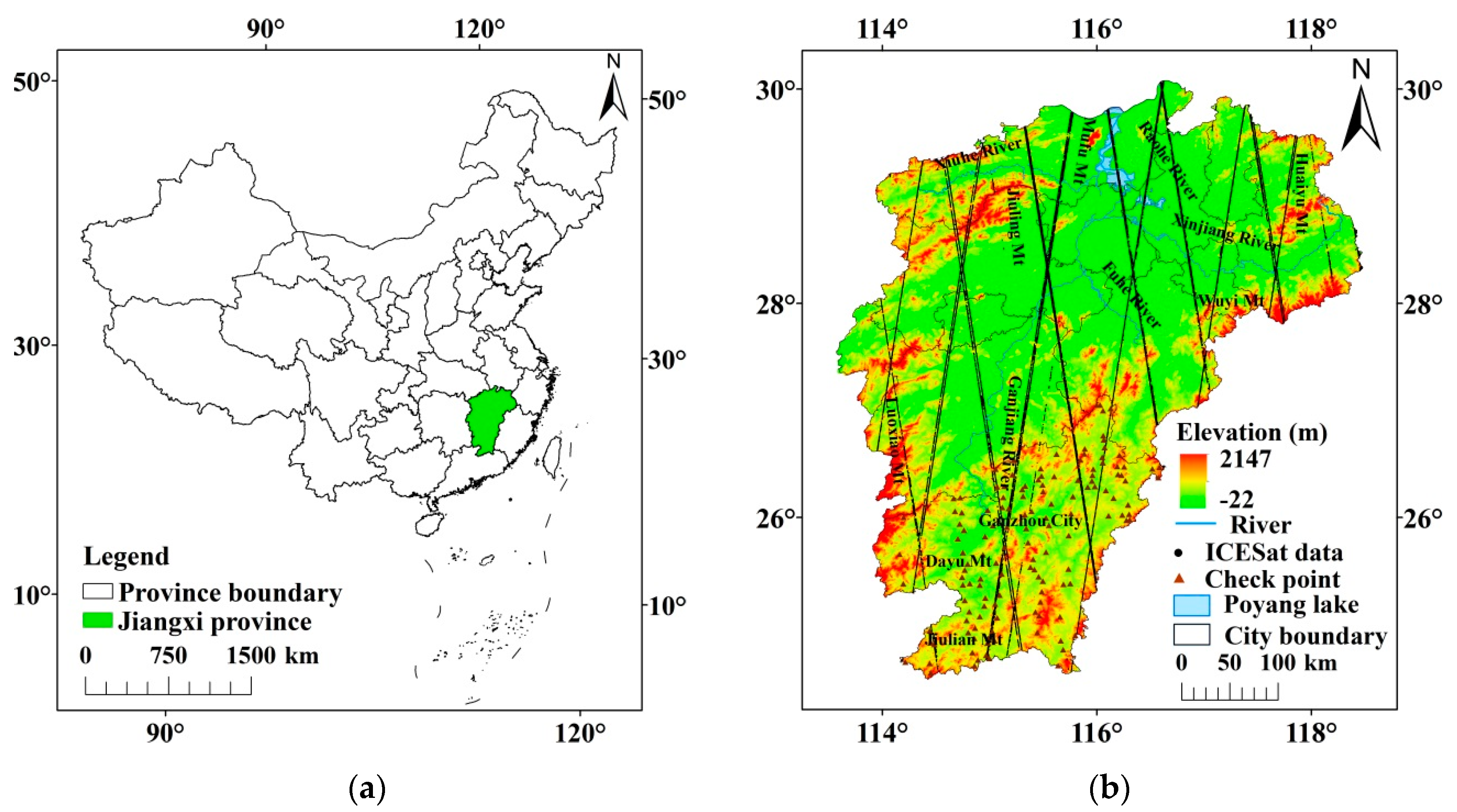
Figure 1. Study site and datasets: (a) location of Jiangxi province, (b) Shuttle Radar Topography Mission (SRTM) digital elevation model (DEM) and Geoscience Laser Altimeter System onboard the Ice, Cloud, and land Elevation Satellite (ICESat/GLAS) data, (c) terrain slope, (d) terrain aspect, (e) terrain relief, and (f) land use.
Remotesensing 12 03435 g001aRemotesensing 12 03435 g001b
Figure 2. Relationship between the heights of ICESat/GLAS data and SRTM DEM.
Remotesensing 12 03435 g002
Figure 3. Structure of back propagation neural network (BPNN) for 3-arc-second SRTM (SRTM3) DEM correction.
Remotesensing 12 03435 g003
Figure 4. Structure of generalized regression NN (GRNN) for SRTM3 DEM correction.
Remotesensing 12 03435 g004
Figure 5. Working flowchart of random forest random forest (RF).
Remotesensing 12 03435 g005
Figure 6. Error histograms of SRTM3 DEM relative to ICESat/GLAS data before and after coregistration.
Remotesensing 12 03435 g006
Figure 7. Relationship between terrain aspect and SRTM3 DEM error relative to ICESat/GLAS data (a) without and (b) with data coregistration.
Remotesensing 12 03435 g007
Figure 8. Influence of terrain slope, relief and elevation classes on the MEs of SRTM3 DEM without and with data coregistration (I: (0–5°) for slope class, (0–100 m) for relief and elevation classes; II: (5–10°) for slope class, (100–200 m) for relief and elevation classes; III: (10–15°) for slope class, (200–300 m) for relief and elevation classes; IV: (15–20°) for slope class, (300–400 m) for relief and elevation classes; V: (>20°) for slope class, (>400 m) for relief and elevation classes. “S”, “R” and “E” stand for slope, relief, and elevation, respectively.).
Remotesensing 12 03435 g008
Figure 9. Influence of terrain slope, relief and elevation classes on the RMSEs of SRTM3 DEM without and with data coregistration (I: (0–5°) for slope class, (0–100 m) for relief and elevation classes; II: (5–10°) for slope class, (100–200 m) for relief and elevation classes; III: (10–15°) for slope class, (200–300 m) for relief and elevation classes; IV: (15–20°) for slope class, (300–400 m) for relief and elevation classes; V: (>20°) for slope class, (>400 m) for relief and elevation classes. “S”, “R” and “E” stand for slope, relief and elevation, respectively.).
Remotesensing 12 03435 g009
Figure 10. (a) ME and (b) RMSE of SRTM3 DEM under different land uses without and with data coregistration (m).
Remotesensing 12 03435 g010
Figure 11. (a) Original SRTM3 DEM, (b) DEM corrected by MLR, (c) DEM corrected by RF, and (d) RF-based DEM minus MLR-based DEM.
Remotesensing 12 03435 g011
Table 1. Mean errors (MEs) and root mean square errors (RMSEs) of SRTM3 DEM without and with data coregistration under different classes of the influence factors.
Influence FactorsClassesME (m)RMSE (m)
WithoutWithWithoutWith
Slope (°)0–5−1.6810.3695.5895.013
5–10−2.153−0.25312.46311.104
10–15−2.632−0.80215.33213.104
15–20−2.653−0.37217.13514.143
>20−2.597−0.39419.52815.825
Relief (m)0–100−1.6920.3715.5254.826
100–200−1.970−0.00512.15810.627
200–300−2.750−0.75314.72812.677
300–400−2.352−0.28915.94413.578
>400−2.574−0.60718.05314.826
Elevation (m)0–100−1.8040.1825.6114.907
100–200−2.221−0.29911.85910.375
200–300−2.517−0.52214.35112.472
300–400−1.5740.31615.15013.002
>400−2.543−0.18416.66013.880
Land useCultivated land−2.550−0.2826.9805.752
Forest cover−2.027−0.11713.84311.879
Grassland−1.7510.09610.7939.231
Water area−0.6951.5083.9253.925
Built-up area−2.0360.0704.9823.532
Unused land−1.3290.6861.7821.316
Table 2. Performance comparison between the correction models for SRTM3 DEM with and without data coregistration relative to ICESat/GLAS data. 3CM represents the three dimensional (3D) coregistration method and MLR represents multiple linear regression.
ModelsME (m)RMSE (m)Computing Cost (s)
WithoutWithWithoutWith
SRTM3 −2.079−0.06111.74010.047-
3CM-−0.061-10.0470.598
MLR−0.045−0.04210.3459.5010.120
BPNN−0.029−0.0039.7939.46710.633
GRNN−0.245−0.04711.45210.3799.594
RF−0.168−0.04110.4299.2113964.742
Table 3. Accuracy assessment of the RF-enhanced DEMs with and without data coregistration relative to GNSS points (m).
Data CoregistrationMERMSE
Without−0.69011.951
With−0.17610.977
Publisher’s Note: MDPI stays neutral with regard to jurisdictional claims in published maps and institutional affiliations.