Modeling Spatial Flood using Novel Ensemble Artificial Intelligence Approaches in Northern Iran

 , ,
, ,  ,
,  and
and
Abstract

1. Introduction
2. Materials and Methods
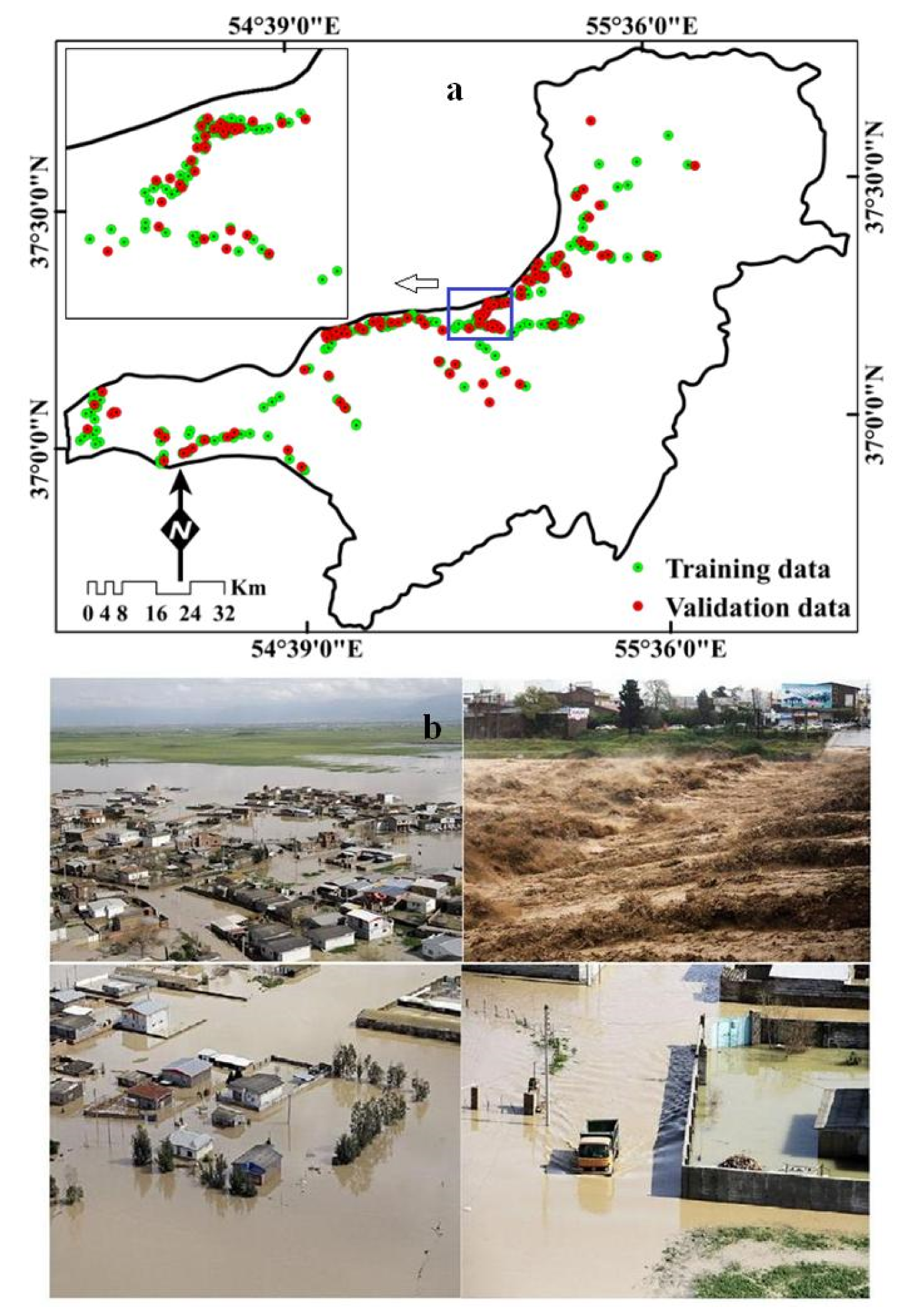
2.1. Description of the Study Area
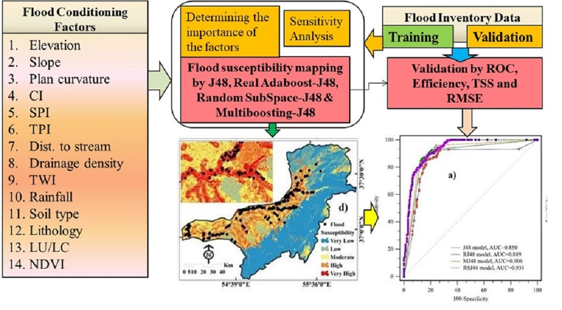
2.2. Methodology
2.3. Database
2.3.1. Flood Inventory Map (FIM)
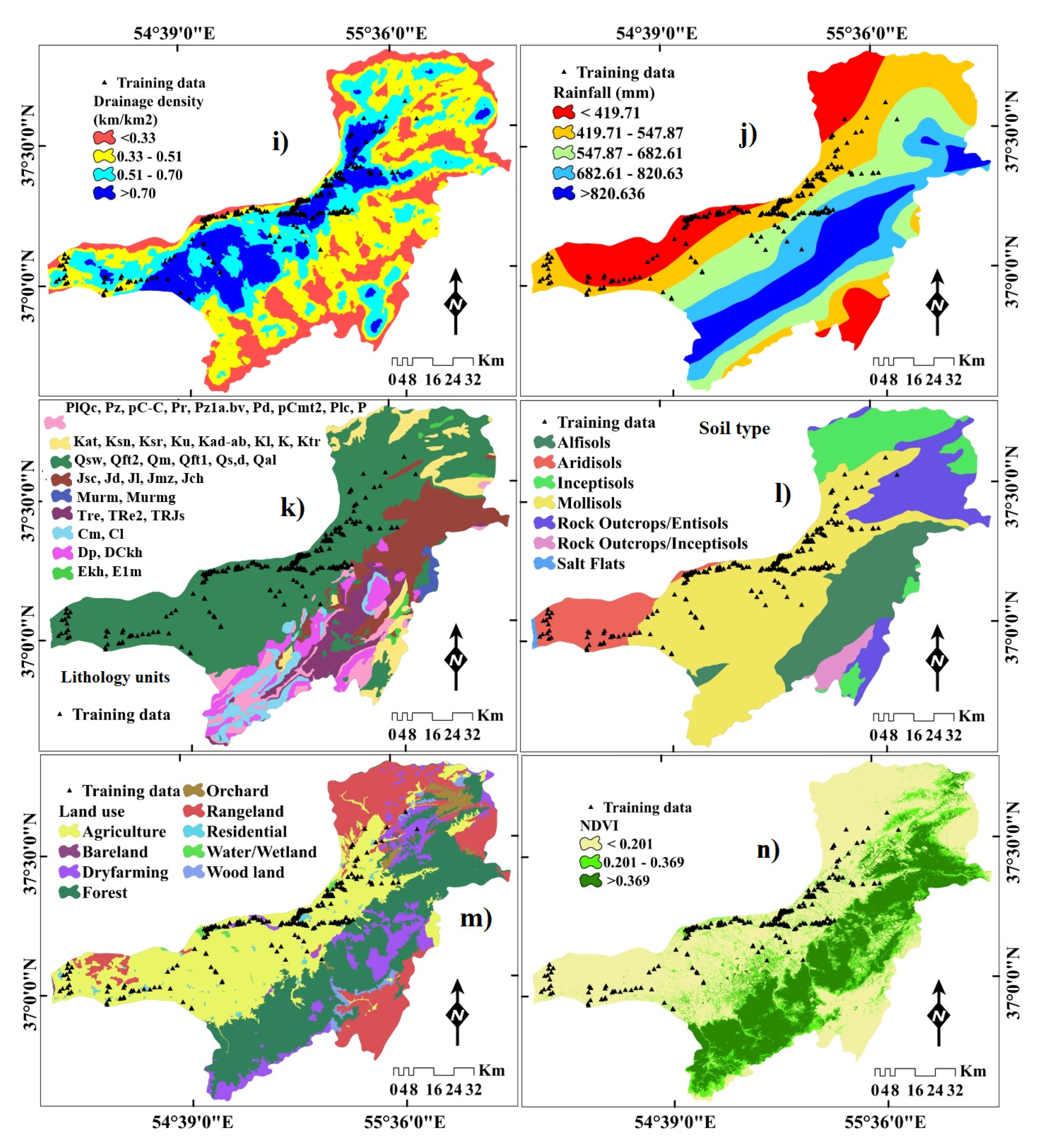
2.3.2. Generating Flood Conditioning Factors (FCFs)
2.4. Multicollinearity Test of Effective Factors
2.5. Analysis of the Relationship between FCFs and Flood Occurrences Using the Frequency Ratio (FR) Model
2.6. Flood Susceptibility Spatial Modeling using Machine Learning Ensemble Methods
2.6.1. J48 Decision Tree
2.6.2. Real AdaBoost
2.6.3. Random Subspace
2.6.4. MultiBoosting
2.7. Model Validation Techniques
2.8. Sensitivity Analysis (SA)
3. Results
3.1. Considering Multicollinearity of Effective Factors
3.2. Spatial Relationship between Flood Probability and FCFs
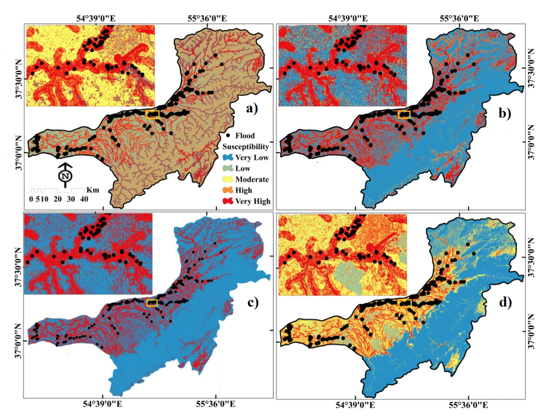
3.3. Flood Susceptibility Models (FSMs)
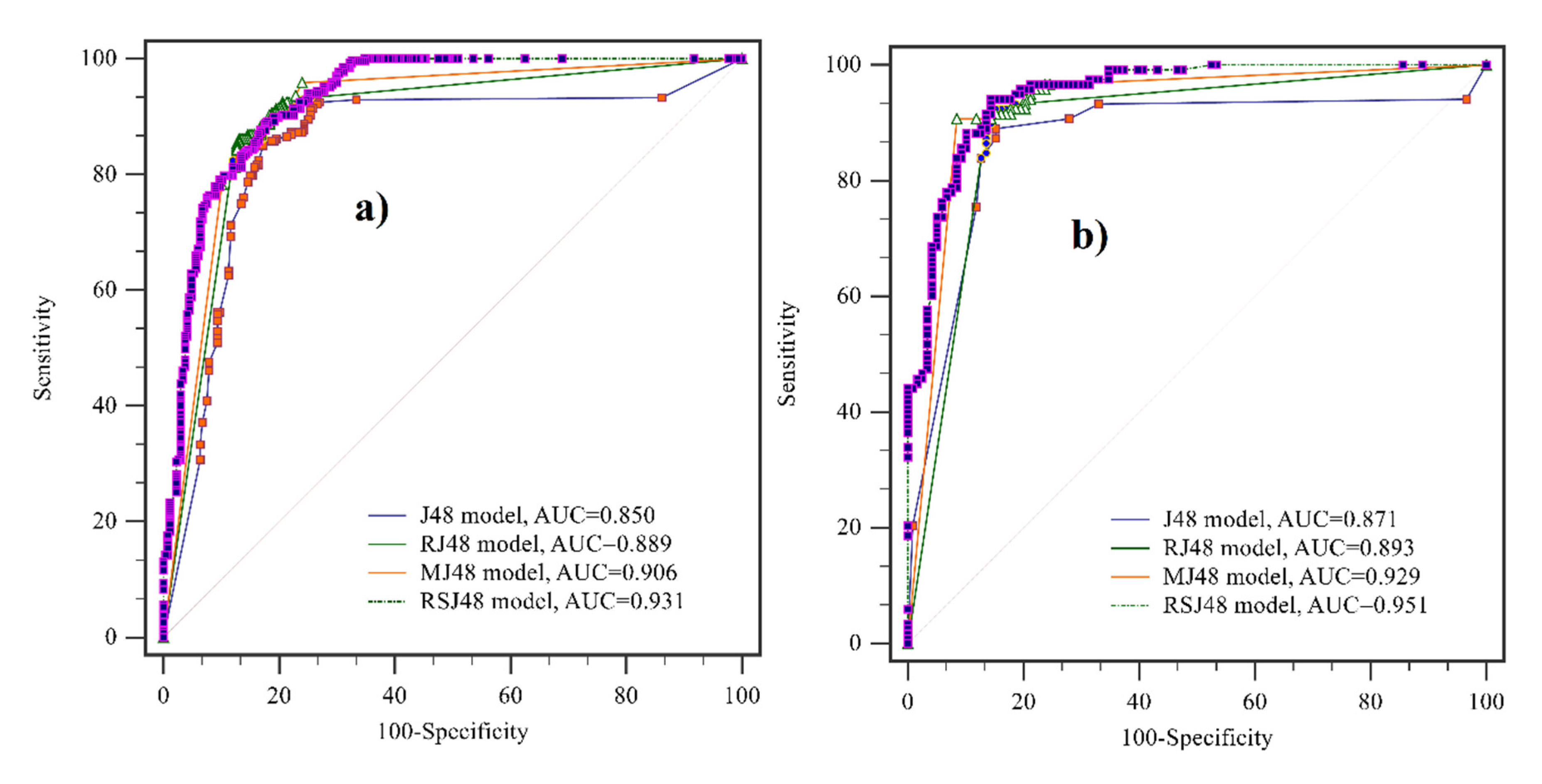
3.4. Validation of Machine Learning Ensemble Models
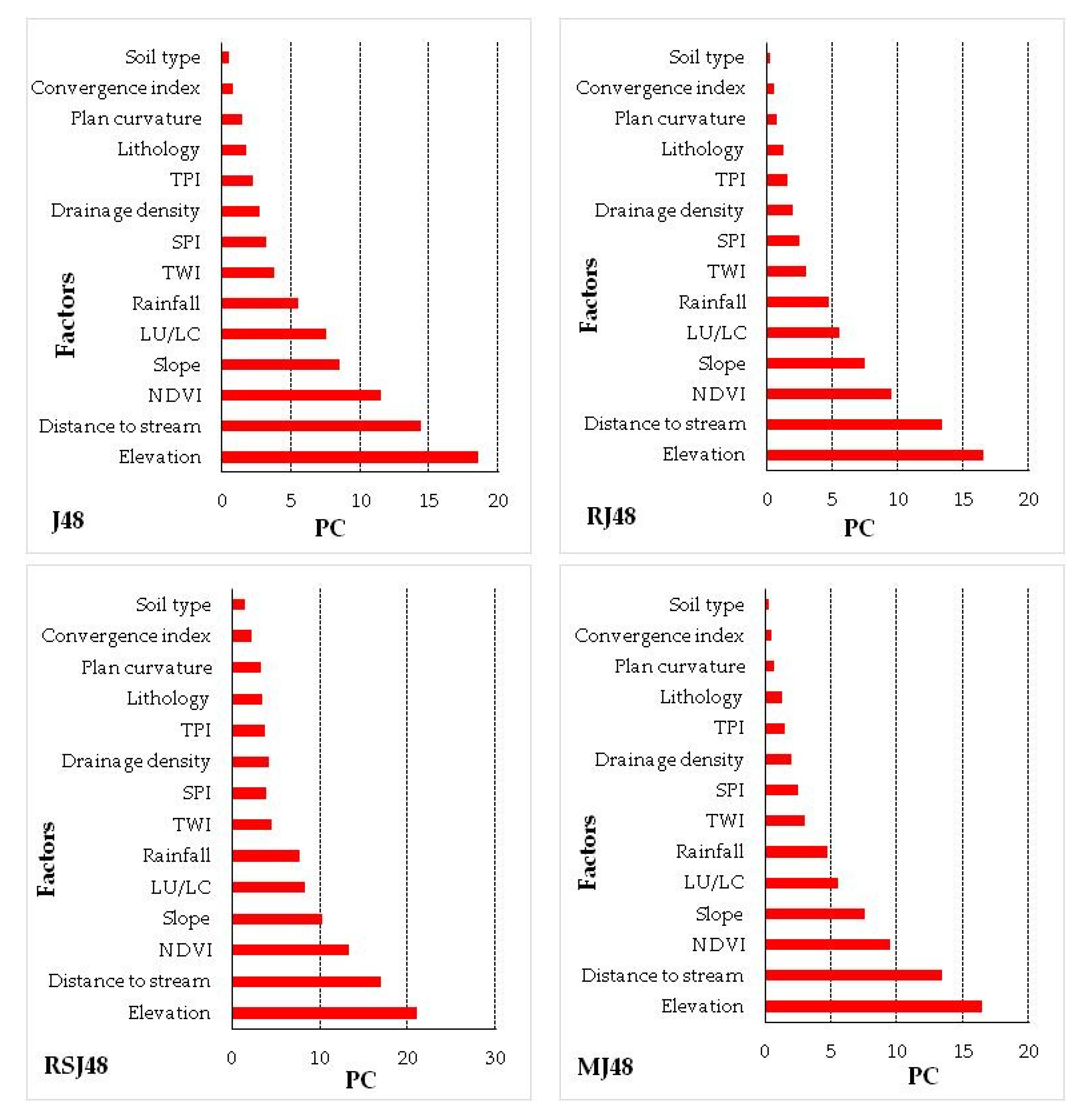
3.5. Sensitivity Analysis
4. Discussion
4.1. Model Performance and Comparison
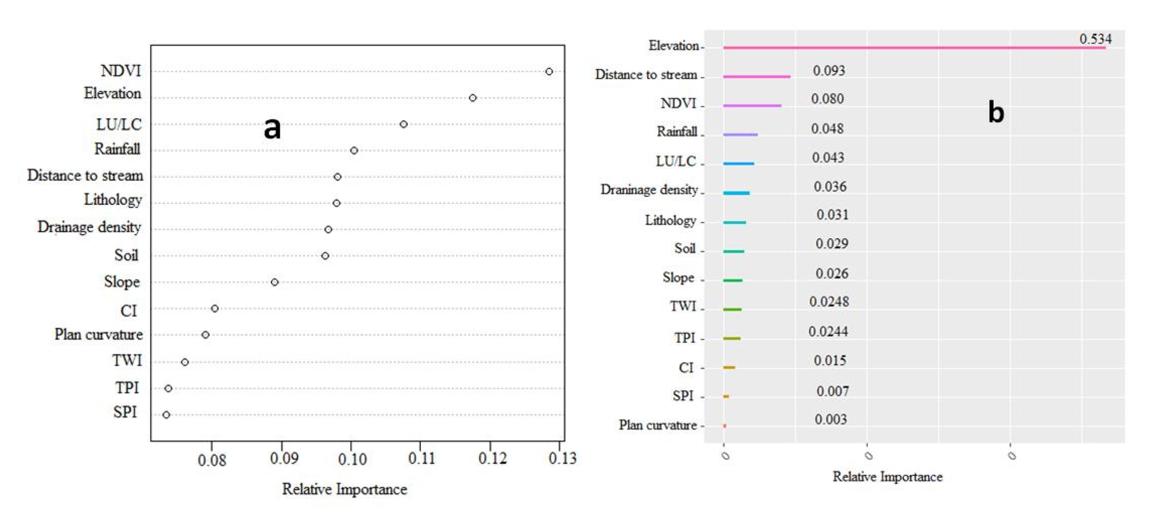
4.2. Factor Contribution Analysis
5. Conclusions
Supplementary Materials
Author Contributions
Funding
Acknowledgments
Conflicts of Interest
References
- Asgharpour, S.E.; Ajdari, B.A. Case Study on Seasonal Floods in Iran, Watershed of Ghotour Chai Basin. Procedia Soc. Behav. Sci. 2011, 19, 556–566. [Google Scholar] [CrossRef]
- Keesstra, S.D. Impact of natural reforestation on floodplain sedimentation in the Dragonja basin, SW Slovenia. Earth Surf. Process. Landf. J. Br. Geomorphol. Res. Group 2007, 32, 49–65. [Google Scholar] [CrossRef]
- Vinet, F. Geographical analysis of damage due to flash floods in southern France: The cases of 12–13 November 1999 and 8–9 September 2002. Appl. Geogr. 2008, 28, 323–336. [Google Scholar] [CrossRef]
- Gharaibeh, A.A.; Zu’bi, A.; Esra’a, M.; Abuhassan, L.B. Amman (City of Waters); Policy, Land Use, and Character Changes. Land 2019, 8, 195. [Google Scholar] [CrossRef]
- Adnan, M.S.G.; Dewan, A.; Zannat, K.E.; Abdullah, A.Y.M. The use of watershed geomorphic data in flash flood susceptibility zoning: A case study of the Karnaphuli and Sangu river basins of Bangladesh. Nat. Hazards 2019, 99, 425–448. [Google Scholar] [CrossRef]
- Hirabayashi, Y.; Mahendran, R.; Koirala, S.; Konoshima, L.; Yamazaki, D.; Watanabe, S.; Kim, H.; Kanae, S. Global flood risk under climate change. Nat. Clim. Chang. 2013, 3, 816. [Google Scholar] [CrossRef]
- CRED; UNISDR. The Human Cost of Weather-Related Disasters, 1995–2015; United Nations: Geneva, Switzerland, 2015.
- Casale, R.; Margottini, C. Floods and Landslides, Integrated Risk Assessment, Integrated Risk Assessment; with 30 Tables; Springer Science & Business Media: Berlin, Germany, 1999. [Google Scholar]
- Smith, K. Environmental Hazards, Assessing Risk and Reducing Disaster; Routledge: Abingdon, UK, 2013. [Google Scholar]
- Paul, G.C.; Saha, S.; Hembram, T.K. Application of the GIS-Based Probabilistic Models for Mapping the Flood Susceptibility in Bansloi Sub-basin of Ganga-Bhagirathi River and Their Comparison. Remote Sens. Earth Syst. Sci. 2019, 15, 120–146. [Google Scholar] [CrossRef]
- Adnan, M.S.G.; Talchabhadel, R.; Nakagawa, H.; Hall, J.W. The potential of Tidal River Management for flood alleviation in South Western Bangladesh. Sci. Total Environ. 2020, 731, 138747. [Google Scholar] [CrossRef]
- Keesstra, S.D.; Bouma, J.; Wallinga, J.; Tittonell, P.; Smith, P.; Bardgett, R.D. The significance of soils and soil science towards realization of the United Nations Sustainable Development Goals. Soil 2016, 2, 111–128. [Google Scholar] [CrossRef]
- Keesstra, S.; Mol, G.; de Leeuw, J.; Okx, J.; de Cleen, M.; Visser, S. Soil-related sustainable development goals: Four concepts to make land degradation neutrality and restoration work. Land 2018, 7, 133. [Google Scholar] [CrossRef]
- Visser, S.; Keesstra, S.; Maas, G.; De Cleen, M. Soil as a Basis to Create Enabling Conditions for Transitions Towards Sustainable Land Management as a Key to Achieve the SDGs by 2030. Sustainability 2019, 11, 6792. [Google Scholar] [CrossRef]
- Algeria: State Owned Reinsurer Shows Strong Technical Results, Good Investment Returns. Available online: https://www.meinsurancereview.com/News/View-NewsLetterArticle?id=46352&Type=MiddleEast (accessed on 20 September 2019).
- Norouzi, G.; Taslimi, M. The impact of flood damages on production of Iran’s agricultural sector. Middle East J. Sci. Res. 2012, 12, 921–926. [Google Scholar]
- Jannati, H. History of the Devastating Floods in Iran. Political Studies and Research Institute 593 of Iran, pr 12. 2019. Available online: http//ir-psri.com/?Page=ViewNews&NewsID=6283 (accessed on 20 September 2019).
- Safaripour, M.; Monavari, M.; Zare, M.; Abedi, Z.; Gharagozlou, A. Flood Risk Assessment Using GIS (Case Study, Golestan Province, Iran). Pol. J. Environ. Stud. 2012, 21, 1817–1824. [Google Scholar]
- Mosavi, A.; Ozturk, P.; Chau, K.W. Flood Prediction Using Machine Learning Models: Literature Review. Water 2018, 10, 1536. [Google Scholar] [CrossRef]
- Kauffeldt, A.; Wetterhall, F.; Pappenberger, F.; Salamon, P.; Thielen, J. Technical review of large-scale hydrological models for implementation in operational flood forecasting schemes on continental level. Environ. Model. Softw. 2016, 75, 68–76. [Google Scholar] [CrossRef]
- Devia, G.K.; Ganasri, B.P.; Dwarakish, G.S. A Review on Hydrological Models. Aquat. Procedia 2015, 4, 1001–1007. [Google Scholar] [CrossRef]
- Chourushi, S.; Lodha, P.; Prakash, I. A Critical Review of Hydrological Modeling Practices for Flood Management. Pramana Res. J. 2019, 9, 352–362. [Google Scholar]
- Sanz-Ramos, M.; Amengual, A.; Bladé Castellet, E.; Romero, R.; Roux, H. Flood forecasting using a coupled hydrological and hydraulic model (based on FVM) and highresolution meteorological model. E3S Web Conf. 2018, 40, 06028. [Google Scholar] [CrossRef]
- Unduche, F.; Tolossa, H.; Senbeta, D.; Zhu, E. Evaluation of four hydrological models for operational flood forecasting in a Canadian Prairie watershed. Hydrol. Sci. J. 2018, 63, 1133–1149. [Google Scholar] [CrossRef]
- Costabile, P.; Macchione, F. Enhancing river model set-up for 2-D dynamic flood modelling. Environ. Model. Softw. 2015, 67, 89–107. [Google Scholar] [CrossRef]
- Fawcett, R.; Stone, R.A. Comparison of two seasonal rainfall forecasting systems for Australia. Aust. Meteorol. Oceanogr. J. 2010, 60, 15–24. [Google Scholar] [CrossRef]
- Arabameri, A.; Karimi-Sangchini, E.; Chandra Pal, S.; Saha, A.; Chowdhuri, I.; Lee, S.; Tien Bui, D. Novel Credal Decision Tree-Based Ensemble Approaches for Predicting the Landslide Susceptibility. Remote Sens. 2020, 12, 3389. [Google Scholar] [CrossRef]
- Ji, J.; Choi, C.; Yu, M.; Yi, J. Comparison of a data-driven model and a physical model for flood forecasting. WIT Trans. Ecol. Environ. 2012, 159, 133–142. [Google Scholar] [CrossRef]
- Nampak, H.; Pradhan, B.; Manap, M.A. Application of GIS based data driven evidential belief function model to predict groundwater potential zonation. J. Hydrol. 2014, 513, 283–300. [Google Scholar] [CrossRef]
- Tehrany, M.S.; Pradhan, B.; Jebur, M.N. Spatial prediction of flood susceptible areas using rule based decision tree (DT) and a novel ensemble bivariate and multivariate statistical models in GIS. J. Hydrol. 2013, 11, 69–79. [Google Scholar] [CrossRef]
- Youssef, A.M.; Pradhan, B.; Sefry, S.A. Flash flood susceptibility assessment in Jeddah city (Kingdom of Saudi Arabia) using bivariate and multivariate statistical models. Environ. Earth Sci. 2016, 75, 12. [Google Scholar] [CrossRef]
- Hong, H.; Liu, J.; Bui, D.T.; Pradhan, B.; Acharya, T.D.; Pham, B.T. Landslide susceptibility mapping using J48 decision tree with AdaBoost, bagging and rotation forest ensembles in the Guangchang area (China). Catena 2018, 163, 399–413. [Google Scholar] [CrossRef]
- Hong, H.; Tsangaratos, P.; Ilia, I.; Liu, J.; Zhu, A.X.; Chen, W. Application of fuzzy weight of evidence and datamining techniques in construction of flood susceptibility map of Poyang County, China. Sci. Total Environ. 2018, 625, 575–588. [Google Scholar] [CrossRef]
- Tien Bui, D.; Pradhan, B.; Nampak, H.; Bui, Q.T.; Tran, Q.A.; Nguyen, Q.P. Hybrid artificial intelligence approach based on neural fuzzy inference model and meta heuristic optimization for flood susceptibility modeling in a high-frequency tropical cyclone area using GIS. J. Hydrol. 2016, 540, 317–330. [Google Scholar] [CrossRef]
- Tehrany, M.S.; Pradhan, B.; Jebur, M.N. Flood susceptibility analysis and its verification using a novel ensemble support vector machine and frequency ratio method. Stoch. Environ. Res. Risk Assess. 2015, 29, 1149–1165. [Google Scholar] [CrossRef]
- Tehrany, M.S.; Kumar, L. The application of a Dempster–Shafer-based evidential belief function in flood susceptibility mapping and comparison with frequency ratio and logistic regression methods. Environ. Earth Sci. 2018, 77, 490. [Google Scholar] [CrossRef]
- Arabameri, A.; Rezaei, K.; Cerdà, A.; Conoscenti, C.; Kalantari, Z. A comparison of statistical methods and multi-criteria decision making to map flood hazard susceptibility in Northern Iran. Sci. Total Environ. 2019, 660, 443–458. [Google Scholar] [CrossRef] [PubMed]
- Radmehr, A.; Araghinejad, S. Developing strategies for urban flood management of Tehran city using SMCDM and ANN. J. Comput. Civ. Eng. 2014, 28, 05014006. [Google Scholar] [CrossRef]
- Chen, Y.R.; Yeh, C.H.; Yu, B. Integrated application of the analytic hierarchy process and the geographic information system for flood risk assessment and flood plain management in Taiwan. Nat. Hazards 2011, 59, 1261–1276. [Google Scholar] [CrossRef]
- Stefanidis, S.; Stathis, D. Assessment of flood hazard based on natural and anthropogenic factors using analytic hierarchy process (AHP). Nat. Hazards 2013, 68, 569–585. [Google Scholar] [CrossRef]
- Zou, Q.; Zhou, J.; Zhou, C.; Song, L.; Guo, J. Comprehensive flood risk assessment based on set pair analysis-variable fuzzy sets model and fuzzy AHP. Stoch. Environ. Res. Risk Assess. 2013, 27, 525–546. [Google Scholar] [CrossRef]
- Kazakis, N.; Kougias, I.; Patsialis, T. Assessment of flood hazard areas at a regional scale using an index-based approach and Analytical Hierarchy Process, Application in Rhodope–Evros region, Greece. Sci. Total Environ. 2015, 538, 555–563. [Google Scholar] [CrossRef]
- Rahmati, O.; Pourghasemi, H.R.; Zeinivand, H. Flood susceptibility mapping using frequency ratio and weights-of-evidence models in the Golastan Province, Iran. Geocarto Int. 2016, 31, 42–70. [Google Scholar] [CrossRef]
- Lee, S.; Kim, Y.S.; Oh, H.J. Application of a weights-of-evidence method and GIS to regional groundwater productivity potential mapping. J. Environ. Manag. 2012, 96, 91–105. [Google Scholar] [CrossRef]
- Rahmati, O.; Nazari Samani, A.; Mahmoodi, N.; Mahdavi, M. Assessment of the contribution of N-fertilizers to nitrate pollution of groundwater in western Iran (case study, Ghorveh–DehgelanArquifer). Water Qual. Expo. Health 2015, 7, 143–151. [Google Scholar] [CrossRef]
- Arabameri, A.; Chen, W.; Blaschke, T.; Tiefenbacher, J.P.; Pradhan, B.; Bui, D.T. Gully Head-Cut Distribution Modeling Using Machine Learning Methods—A Case Study of N.W. Iran. Water 2020, 12, 16. [Google Scholar] [CrossRef]
- Arabameri, A.; Cerda, A.; Pradhan, B.; Tiefenbacher, J.P.; Lombardo, L.; Bui, D.T. A methodological comparison of head-cut based gully erosion susceptibility models: Combined use of statistical and artificial intelligence. Geomorphology 2020, 107136. [Google Scholar] [CrossRef]
- Arabameri, A.; Lee, S.; Tiefenbacher, J.P.; Ngo, P.T.T. Novel Ensemble of MCDM-Artificial Intelligence Techniques for Groundwater-Potential Mapping in Arid and Semi-Arid Regions (Iran). Remote Sens. 2020, 12, 490. [Google Scholar] [CrossRef]
- Arabameri, A.; Blaschke, T.; Pradhan, B.; Pourghasemi, H.R.; Tiefenbacher, J.P.; Bui, D.T. Evaluation of Recent Advanced Soft Computing Techniques for Gully Erosion Susceptibility Mapping: A Comparative Study. Sensors 2020, 20, 335. [Google Scholar] [CrossRef]
- Pham, B.T.; Tien Bui, D.; Prakash, I.; Dholakia, M.B. Rotation forest fuzzy rule-based classifier ensemble for spatial prediction of landslides using GIS. Nat. Hazards 2016, 83, 97–127. [Google Scholar] [CrossRef]
- Althuwaynee, O.F.; Pradhan, B.; Lee, S. Application of an evidential belief function model in landslide susceptibility mapping. Comput. Geosci. 2012, 44, 120–135. [Google Scholar] [CrossRef]
- Chen, W.; Shirzadi, A.; Shahabi, H.; Ahmad, B.B.; Zhang, S.; Hong, H. A novel hybrid artificial intelligence approach based on the rotation forest ensemble and naive Bayes tree classifiers for a landslide susceptibility assessment in Langao County, China. Geomat. Nat. Hazards Risk 2017, 8, 1955–1977. [Google Scholar] [CrossRef]
- Tien Bui, D.; Tuan, T.A.; Hoang, N.-D.; Thanh, N.Q.; Nguyen, D.B.; Van Liem, N. Spatial prediction of rainfall-induced landslides for the Lao Cai area (Vietnam) using a hybrid intelligent approach of least squares support vector machines inference model and artificial bee colony optimization. Landslides 2017, 14, 447–458. [Google Scholar] [CrossRef]
- Kordestani, M.D.; Naghibi, S.A.; Hashemi, H.; Ahmadi, K.; Kalantar, B.; Pradhan, B. Groundwater potential mapping using a novel data-mining ensemble model. J. Hydrol. 2019, 27, 211–224. [Google Scholar] [CrossRef]
- Rahmati, O.; Naghibi, S.A.; Shahabi, H.; Bui, D.T.; Pradhan, B.; Azareh, A.; Melesse, A.M. Groundwater spring potential modelling, Comprising the capability and robustness of three different modeling approaches. J. Hydrol. 2018, 565, 248–261. [Google Scholar] [CrossRef]
- Hosseini, F.S.; Choubin, B.; Mosavi, A. Flash-flood hazard assessment using ensembles and Bayesian-based machine learning models: Application of the simulated annealing feature selection method. Sci. Total Environ. 2020, 711, 135161. [Google Scholar] [CrossRef]
- Janizadeh, S.; Avand, M.; Jaafari, A. Prediction Success of Machine Learning Methods for Flash Flood Susceptibility Mapping in the Tafresh Watershed, Iran. Sustainability 2019, 11, 5426. [Google Scholar] [CrossRef]
- Edwards, P.K.; Duhon, D.; Shergill, S. Real AdaBoost, Boosting for Credit Scorecards and Similarity to WOE Logistic Regression; Scotiabank: Toronto, ON, Canada, 2019; pp. 1323–2017. [Google Scholar]
- Tao, D.; Tang, X.; Li, X.; Wu, X. Asymmetric bagging and random subspace for support vector machines-based relevance feedback in image retrieval. IEEE Trans. Pattern Anal. Mach. Intell. 2006, 28, 1088–1099. [Google Scholar] [PubMed]
- Nanni, L.; Lumini, A. Random subspace for an improved biohashing for face authentication. Pattern Recogn. Lett. 2008, 29, 295–300. [Google Scholar] [CrossRef]
- Zhang, X.; Jia, Y. A linear discriminant analysis framework based on random subspace for face recognition. Pattern Recognit. 2007, 40, 2585–2591. [Google Scholar] [CrossRef]
- Zhu, Y.; Liu, J.; Chen, S. Semi-random subspace method for face recognition. Image Vis. Comput. 2009, 27, 1358–1370. [Google Scholar] [CrossRef]
- Hong, H.; Liu, J.; Zhu, A.X.; Shahabi, H.; Pham, B.T.; Chen, W.; Pradhan, B.; Bui, D.T. A novel hybrid integration model using support vector machines and random subspace for weather-triggered landslide susceptibility assessment in the Wuning area (China). Environ. Earth Sci. 2017, 76, 652. [Google Scholar] [CrossRef]
- Webb, G.I. MultiBoosting, a technique for combining boosting and wagging. Mach. Learn. 2000, 40, 159–196. [Google Scholar] [CrossRef]
- IRIMO. Summary Reports of Iran’s Extreme Climatic Events. Ministry of Roads and Urban Development, Iran Meteorological Organization. 2012. Available online: www.cri.ac.ir (accessed on 20 September 2019).
- GSI. Geology Survey of Iran. 1997. Available online: http//www.gsi.ir/Main/Lang_en/index.html (accessed on 20 September 2019).
- Donya-e-Eqtesad. 2019. Available online: https//www.donya-e-eqtesad.com/fa/tiny/news-5863511460 (accessed on 20 September 2019).
- Hasan, M.K.; Kumar, L.; Gopalakrishnan, T. Inundation modelling for Bangladeshi coasts usingdownscaled and bias-corrected temperature. Clim. Risk Manag. 2020, 27, 100207. [Google Scholar] [CrossRef]
- Gesch, D.; Oimoen, M.; Zhang, Z.; Meyer, D.; Danielson, J. Validation of the ASTER global digital elevation model version 2 over the conterminous United States. Int. Arch. Photogramm. Remote Sens. Spat. Inf. Sci. 2012, B4, 281–286. [Google Scholar]
- Arabameri, A.; Saha, S.; Chen, W.; Roy, J.; Pradhan, B.; Bui, D.T. Flash flood susceptibility modelling using functional tree and hybrid ensemble techniques. J. Hydrol. 2020, 587, 125007. [Google Scholar] [CrossRef]
- Arabameri, A.; Pradhan, B.; Bui, D.T. Spatial modelling of gully erosion in the Ardib River Watershed using three statistical-based techniques. Catena 2020, 190, 104545. [Google Scholar] [CrossRef]
- Zakerinejad, R.; Maerker, M. Prediction of gully erosion susceptibilities using detailed terrain analysis and maximum entropy modeling: A case study in the Mazayejan Plain, Southwest Iran. Suppl. Geogr. Fis. Din. Quat. 2014, 37, 67–76. [Google Scholar]
- Bui, D.T.; Ho, T.C.; Pradhan, B.; Pham, B.T.; Nhu, V.H.; Revhaug, I. GIS-based modeling of rainfall-induced landslides using data mining-based functional trees classifier with AdaBoost, Bagging, and MultiBoost ensemble frameworks. Environ. Earth Sci. 2016, 75, 1101. [Google Scholar]
- Khosravi, K.; Pourghasemi, H.R.; Chapi, K.; Bahri, M. Flash flood susceptibility analysis and its mapping using different bivariate models in Iran: A comparison between Shannon’s entropy, statistical index, andweighting factor models. Environ. Monit. Assess. 2016, 188, 656. [Google Scholar] [CrossRef] [PubMed]
- Meraj, G.; Romshoo, S.A.; Yousuf, A.R.; Altaf, S.; Altaf, F. Assessing the influence of watershed characteristics on the flood vulnerability of Jhelum basin in Kashmir Himalaya. Nat. Hazards 2015, 77, 153–175. [Google Scholar] [CrossRef]
- Khosravi, K.; Nohani, E.; Maroufinia, E.; Pourghasemi, H.R. A GIS-based flood susceptibility assessment and its mapping in Iran, a comparison between frequency ratio and weights-of-evidence bivariate statistical models with multi-criteria decision-making technique. Nat. Hazards 2016, 83, 947–987. [Google Scholar] [CrossRef]
- Botzen, W.J.W.; Aerts, J.C.J.H.; van den Bergh, J.C.J.M. Individual preferences for reducing flood risk to near zero through elevation. Mitig. Adapt. Strateg. Glob. Chang. 2012, 2, 229–244. [Google Scholar] [CrossRef]
- Kirkby, M.J.; Beven, K.J. A physically based, variable contributing area model of basin hydrology. Hydrol. Sci. Bull. 1979, 24, 43–69. [Google Scholar]
- Gokceoglu, C.; Sonmez, H.; Nefeslioglu, H.A.; Duman, T.Y.; Can, T. The 17 March 2005 Kuzulu landslide (Sivas, Turkey) and landslide-susceptibility map of its near vicinity. Eng. Geol. 2005, 81, 65–83. [Google Scholar] [CrossRef]
- Riley, S.J.; De Gloria, S.D.; Elliot, R. A terrain ruggedness index that quantifies topographic heterogeneity. Intermt. J. Sci. 1999, 5, 23–27. [Google Scholar]
- Gallant, J.C.; Wilson, J.P. Primary topographic attributes. In Terrain Analysis, Principles and Applications; Wilson, J.P., Gallant, J.C., Eds.; Wiley: New York, NY, USA, 2000; pp. 51–85. [Google Scholar]
- Weiss, A. Topographic position and landforms analysis. In Proceedings of the Poster Presentation, ESRI User Conference, San Diego, CA, USA, 9 July 2001; Volume 200. [Google Scholar]
- Grohmann, C.H.; Riccomini, C. Comparison of roving-window and search-window techniques for characterising landscape morphometry. Comput. Geosci. 2009, 35, 2164–2169. [Google Scholar] [CrossRef]
- Moore, I.D.; Grayson, R.B.; Ladson, A.R. Digital terrain modelling: A review of hydrological, geomorphological, and biological applications. Hydrol. Process. 1991, 5, 3–30. [Google Scholar] [CrossRef]
- Kiss, R. Determination of drainage network in digital elevation model, utilities and limitations. J. Hung. Geo-Math. 2004, 2, 16–29. [Google Scholar]
- Khosravi, K.; Pham, B.T.; Chapi, K.; Shirzadi, A.; Shahabi, H.; Revhaug, I. A comparative assessment of decision trees algorithms for flash flood susceptibility modeling at Haraz watershed, northern Iran. Sci. Total Environ. 2018, 627, 744–755. [Google Scholar] [CrossRef]
- Opperman, J.J.; Galloway, G.E.; Fargione, J.; Mount, J.F.; Richter, B.D.; Secchi, S. Sustainable floodplains through large-scale reconnection to rivers. Science 2009, 3265959, 1487–1488. [Google Scholar] [CrossRef]
- Boer, E.P.; de Beurs, K.M.; Hartkamp, A.D. Kriging and thin plate splines for mapping climate variables. Int. J. Appl. Earth Obs. Geoinf. 2001, 3, 146–154. [Google Scholar] [CrossRef]
- Sajedi-Hosseini, F.; Choubin, B.; Solaimani, K.; Cerdà, A.; Kavian, A. Spatial prediction of soil erosion susceptibility using a fuzzy analytical network process, Application of the fuzzy decision-making trial and evaluation laboratory approach. Land Degrad. Dev. 2018, 29, 3092–3103. [Google Scholar] [CrossRef]
- Lo, C.P.; Yeung, A.K.W. Concepts and Techniques of Geographic Information System; Pearson Education Inc.: Hoboken, NJ, USA, 2002. [Google Scholar]
- Pradhan, B. Flood susceptible mapping and risk area estimation using logistic regression, GIS and remote sensing. J. Spat. Hydrol. 2010, 9, 1–18. [Google Scholar]
- Arabameri, A.; Nalivan, O.A.; Saha, S.; Roy, J.; Pradhan, B.; Tiefenbacher, J.P.; Ngo, P.T.T. Novel Ensemble Approaches of Machine Learning Techniques in Modeling the Gully Erosion Susceptibility. Remote Sens. 2020, 12, 1890. [Google Scholar] [CrossRef]
- Arabameri, A.; Chen, W.; Lombardo, L.; Blaschke, T.; Tien Bui, D. Hybrid Computational Intelligence Models for Improvement Gully Erosion Assessment. Remote Sens. 2020, 12, 140. [Google Scholar] [CrossRef]
- Arabameri, A.; Chen, W.; Loche, M.; Zhao, X.; Li, Y.; Lombardo, L.; Cerda, A.; Pradhan, B.; Bui, D.T. Comparison of machine learning models for gully erosion susceptibility mapping. Geosci. Front. 2020, 11, 1609–1620. [Google Scholar] [CrossRef]
- Roy, J.; Saha, S.; Arabameri, A.; Blaschke, T.; Bui, D.T. A Novel Ensemble Approach for Landslide Susceptibility Mapping (LSM) in Darjeeling and Kalimpong Districts, West Bengal, India. Remote Sens. 2019, 11, 2866. [Google Scholar] [CrossRef]
- Arabameri, A.; Cerda, A.; Rodrigo-Comino, J.; Pradhan, B.; Sohrabi, M.; Blaschke, T.; Bui, D.T. Proposing a Novel Predictive Technique for Gully Erosion Susceptibility Mapping in Arid and Semi-arid Regions (Iran). Remote Sens. 2019, 11, 2577. [Google Scholar] [CrossRef]
- Gayen, A.; Pourghasemi, H.R.; Saha, S.; Keesstra, S.; Bai, S. Gully erosion susceptibility assessment and management of hazard-prone areas in India using different machine learning algorithms. Sci. Total Environ. 2019, 668, 124–138. [Google Scholar] [CrossRef]
- Lee, S.; Pradhan, B. Landslide hazard mapping at Selangor, Malaysia using frequency ratio and logistic regression models. Landslides 2006, 4, 33–41. [Google Scholar] [CrossRef]
- Kaur, G.; Chhabra, A. Improved J48 classification algorithm for the prediction of diabetes. Int. J. Comput. Appl. 2014, 98, 13–17. [Google Scholar] [CrossRef]
- Witten, H.I.; Frank, E.; Mark, A. Hall Data Mining: Practical Machine Learning Tools and Techniques, 3rd ed.; Morgan Kaufmann: Burlington, MA, USA, 2011; p. 664. [Google Scholar]
- Freund, Y.; Schapire, R.E. A decision-theoretic generalization of on-line learning and an application to boosting. J. Comput. Syst. Sci. 1997, 55, 119–139. [Google Scholar] [CrossRef]
- Friedman, H.; Hastie, T.; Tibshirani, R. Additive logistic regression, a statistical view of boosting. Ann. Stat. 2000, 28, 337–407. Available online: https//web.stanford.edu/~hastie/Papers/AdditiveLogisticRegression/alr.pdf (accessed on 25 September 2019). [CrossRef]
- Ho, T.K. Nearest neighbors in random subspaces. In Joint IAPR International Workshops on Statistical Techniques in Pattern Recognition (SPR) and Structural and Syntactic Pattern Recognition (SSPR); Springer: Berlin/Heidelberg, Germany, 1998; pp. 640–648. [Google Scholar]
- Kotsiantis, S. Combining bagging, boosting, rotation forest and random subspace methods. Artif. Intell. Rev. 2011, 35, 223–240. [Google Scholar] [CrossRef]
- Kuncheva, L.I.; Rodrı’guez, J.J.; Plumpton, C.O.; Linden, D.E.; Johnston, S.J. Random subspace ensembles for fMRI classification. IEEE Trans. Med. Imaging 2010, 29, 531–542. [Google Scholar] [CrossRef]
- Mielniczuk, J.; Teisseyre, P. Using random subspace method for prediction and variable importance assessment in linear regression. Comput. Stat. Data Anal. 2014, 71, 725–742. [Google Scholar] [CrossRef]
- Sun, S.; Zhang, C. The selective random subspace predictor for traffic flow forecasting. IEEE Trans. Intell. Transp. Syst. 2007, 8, 367–373. [Google Scholar] [CrossRef]
- Chen, W.; Zhao, X.; Tsangaratos, P.; Shahabi, H.; Ilia, I.; Xue, W.; Wang, X.; Ahmad, B.B. Evaluating the usage of tree-based ensemble methods in groundwater spring potential mapping. J. Hydrol. 2020, 583, 124602. [Google Scholar] [CrossRef]
- Li, Y.; Chen, W. Landslide susceptibility evaluation using hybrid integration of evidential belief function and machine learning techniques. Water 2020, 12, 113. [Google Scholar] [CrossRef]
- Wang, G.; Lei, X.; Chen, W.; Shahabi, H.; Shirzadi, A. Hybrid computational intelligence methods for landslide susceptibility mapping. Symmetry 2020, 12, 325. [Google Scholar] [CrossRef]
- Lei, X.; Chen, W.; Pham, B.T. Performance evaluation of gis-based artificial intelligence approaches for landslide susceptibility modeling and spatial patterns analysis. ISPRS Int. J. Geo-Inform. 2020, 9, 443. [Google Scholar] [CrossRef]
- Chen, X.; Chen, W. Gis-based landslide susceptibility assessment using optimized hybrid machine learning methods. CATENA 2021, 196, 104833. [Google Scholar] [CrossRef]
- Zhao, X.; Chen, W. Gis-based evaluation of landslide susceptibility models using certainty factors and functional trees-based ensemble techniques. Appl. Sci. 2020, 10, 16. [Google Scholar] [CrossRef]
- Chen, W.; Li, Y. Gis-based evaluation of landslide susceptibility using hybrid computational intelligence models. CATENA 2020, 195, 104777. [Google Scholar] [CrossRef]
- Chen, W.; Chen, X.; Peng, J.; Panahi, M.; Lee, S. Landslide susceptibility modeling based on anfis with teaching-learning-based optimization and satin bowerbird optimizer. Geosci. Front. 2021, 12, 93–107. [Google Scholar] [CrossRef]
- Fukuda, S.; De Baets, B.; Waegeman, W.; Verwaeren, J.; Mouton, A.M. Habitat prediction and knowledge extraction for spawning European grayling (Thymallusthymallus L.) using a broad range of species distribution models. Environ. Modell. Softw. 2013, 47, 1–6. [Google Scholar] [CrossRef]
- Saltelli, A.; Chan, K.; Scott, E.M. Sensitivity Analysis; Wiley: New York, NY, USA, 2000. [Google Scholar]
- Crosetto, M.; Tarantola, S. Uncertainty and sensitivity analysis: Tools for GISbased model implementation. Int. J. Geogr. Inf. Sci. 2001, 15, 415–437. [Google Scholar] [CrossRef]
- Ferretti, F.; Saltelli, A.; Tarantola, S. Trends in sensitivity analysis practice in the last decade. Sci. Total Environ. 2016, 568, 666–670. [Google Scholar] [CrossRef] [PubMed]
- Chen, Y.; Yu, J.; Khan, S. Spatial sensitivity analysis of multi-criteria weights in GISbased land suitability evaluation. Environ. Model. Softw. 2010, 25, 1582–1591. [Google Scholar] [CrossRef]
- Lodwick, W.A.; Monson, W.; Svoboda, L. Attribute error and sensitivity analysis of map operations in geographical information systems: Suitability analysis. Int. J. Geogr. Inf. Syst. 1990, 4, 413–428. [Google Scholar] [CrossRef]
- Oh, H.J.; Kim, Y.S.; Choi, J.K.; Park, E.; Lee, S. GIS mapping of regional probabilistic groundwater potential in the area of Pohang City, Korea. J. Hydrol. 2011, 399, 158–172. [Google Scholar] [CrossRef]
- Fenta, A.A.; Kifle, A.; Gebreyohannes, T.; Hailu, G. Spatial analysis of groundwater potential using remote sensing and GIS-based multi-criteria evaluation in Raya Valley, northern Ethiopia. Hydrogeol. J. 2015, 23, 195–206. [Google Scholar] [CrossRef]
- Convertino, M.; Muñoz-Carpena, R.; Chu-Agor, M.L.; Kiker, G.L.; Linkov, I. Untangling drivers of species distributions: Global sensitivity and uncertainty analyses of MAXENT. Environ. Model. Softw. 2014, 51, 296–309. [Google Scholar] [CrossRef]
- Park, N.W. Using maximum entropy modeling for landslide susceptibility mapping with multiple geoenvironmental data sets. Environ. Earth Sci. 2015, 73, 937–949. [Google Scholar] [CrossRef]
- Arabameri, A.; Saha, S.; Roy, J.; Chen, W.; Blaschke, T.; Tien Bui, D. Landslide Susceptibility Evaluation and Management Using Different Machine Learning Methods in The Gallicash River Watershed, Iran. Remote Sens. 2020, 12, 475. [Google Scholar] [CrossRef]
- Arabameri, A.; Pradhan, B.; Lombardo, L. Comparative assessment using boosted regression trees, binary logistic regression, frequency ratio and numerical risk factor for gully erosion susceptibility modelling. Catena 2019, 183, 104223. [Google Scholar] [CrossRef]
- Pham, B.T.; Bui, D.T.; Prakash, I.; Dholakia, M.B. Hybrid integration of Multilayer Perceptron Neural Networks and machine learning ensembles for landslide susceptibility assessment at Himalayan area (India) using GIS. Catena 2017, 149, 52–63. [Google Scholar] [CrossRef]
- Tien Bui, D.; Tien Ho, C.; Revhaug, I.; Pradhan, B.; Duy Nguyen, B. Landslide susceptibility mapping along the national road 32 of Vietnam using GIS-based j48 decision tree classifier and its ensembles. In Cartography from Pole to Pole; Buchroithner, M., Prechtel, N., Burghardt, D., Eds.; Springer: Berlin/Heidelberg, Germany, 2014; pp. 303–317. [Google Scholar]
- Kuncheva, L.I. Combining Pattern Classifiers Methods and Algorithms; Wiley: Chichester, UK, 2004. [Google Scholar]
- Onan, A. On the performance of ensemble learning for automated diagnosis of breast cancer. Artif. Intell. Perspect. Appl. 2015, 347, 119–129. [Google Scholar]
- Robinzonov, N. Advances in Boosting of Temporal and Spatial Models. Ludwig-Maximilians-Universitat München. 2013. Available online: http://edoc.ub.uni-muenchen.de/15338/ (accessed on 20 September 2019).
- Aertsen, W.; Kint, V.; Van Orshoven, J. Evaluation of modelling techniques for forest site productivity prediction in contrasting ecoregions using stochastic multicriteria acceptability analysis (SMAA). Environ. Model. Softw. 2011, 26, 929–937. [Google Scholar] [CrossRef]
- Breiman, L. Arcing Classifiers. Ann. Stat. 1998, 26, 801–849. [Google Scholar] [CrossRef]
- Therneau, T.M.; Atkinson, B.; Ripley, B. RPART: Recursive Partitioning and Regression Trees. R Package Version 2014, 4, 1–8. Available online: http://CRAN.R-project.org/package=rpart (accessed on 20 September 2019).


| Factors | Collinearity Statistics | Factors | Collinearity Statistics |
|---|---|---|---|
| VIF | VIF | ||
| Land Use/Land Cover (LU/LC) | 1.330 | Distance to stream | 1.405 |
| Soil type | 2.070 | Slope | 1.33 |
| Elevation | 4.677 | TWI | 6.876 |
| NDVI | 1.025 | Plan curvature | 2.116 |
| Lithology | 3.864 | TPI | 3.246 |
| CI | 1.218 | Drainage density | 1.521 |
| Rainfall | 1.523 | SPI | 4.21 |
| Factor | Class | Pixels in Domain | Flood Pixels | FR | ||
|---|---|---|---|---|---|---|
| No | % | No | % | |||
| Elevation (m) | <287 | 4,346,424 | 41.05 | 266 | 99.63 | 2.43 |
| 287–784 | 2,168,214 | 20.48 | 1 | 0.37 | 0.02 | |
| 784–1331 | 1,878,667 | 17.74 | 0 | 0 | 0 | |
| 1331–1930 | 1,595,868 | 15.07 | 0 | 0 | 0 | |
| >1930 | 599,235 | 5.66 | 0 | 0 | 0 | |
| Slope (°) | <5.8 | 4,572,709 | 43.21 | 245 | 91.76 | 2.12 |
| 5.8–14.2 | 1,907,632 | 18.03 | 21 | 7.87 | 0.44 | |
| 14.2–22.6 | 1,985,057 | 18.76 | 0 | 0 | 0 | |
| 22.6–32.5 | 1,468,311 | 13.88 | 0 | 0 | 0 | |
| >32.5 | 648,343 | 6.13 | 1 | 0.37 | 0.06 | |
| plan curvature (100/m) | Concave | 4,792,528 | 45.29 | 127 | 47.57 | 1.05 |
| Flat | 966,851 | 9.14 | 28 | 10.49 | 1.15 | |
| Convex | 4,822,674 | 45.57 | 112 | 41.95 | 0.92 | |
| CI (100/m) | <−52.9 | 566,739 | 5.42 | 28 | 10.49 | 1.94 |
| −52.9–−16.07 | 1,913,693 | 18.29 | 63 | 23.60 | 1.29 | |
| −16.07–14.5 | 5,483,516 | 52.42 | 97 | 36.33 | 0.69 | |
| 14.5–50.5 | 2,040,048 | 19.50 | 70 | 26.22 | 1.34 | |
| >50.5 | 456,989 | 4.37 | 9 | 3.37 | 0.77 | |
| SPI | <8.87 | 2,478,650 | 23.64 | 118 | 44.53 | 1.88 |
| 8.87–10.91 | 3,180,547 | 30.33 | 88 | 33.21 | 1.09 | |
| 10.91–12.8 | 3,156,931 | 30.10 | 41 | 15.47 | 0.51 | |
| 12.8–15.7 | 1,367,215 | 13.04 | 9 | 3.40 | 0.26 | |
| >15.7 | 303,841 | 2.90 | 9 | 3.40 | 1.17 | |
| TPI | <−10.98 | 428,583 | 4.05 | 2 | 0.75 | 0.18 |
| −10.98–−3.71 | 1,287,289 | 12.16 | 7 | 2.62 | 0.22 | |
| −3.71–2.34 | 6,565,378 | 62.04 | 240 | 89.89 | 1.45 | |
| 2.34–9.62 | 1,761,349 | 16.64 | 18 | 6.74 | 0.41 | |
| >9.62 | 539,452 | 5.10 | 0 | 0 | 0 | |
| TWI | <5.07 | 4,230,756 | 39.98 | 25 | 9.36 | 0.23 |
| 5.07–7.49 | 4047,824 | 38.25 | 152 | 56.93 | 1.49 | |
| 7.49–11.08 | 1,859,417 | 17.57 | 74 | 27.72 | 1.58 | |
| >11.08 | 444,055 | 4.20 | 16 | 5.99 | 1.43 | |
| Drainage density (km/km2) | <0.33 | 2,292,946 | 21.67 | 29 | 10.86 | 0.50 |
| 0.33–0.51 | 3,948,804 | 37.32 | 91 | 34.08 | 0.91 | |
| 0.51–0.7 | 2,702,068 | 25.53 | 86 | 32.21 | 1.26 | |
| >0.7 | 1,638,253 | 15.48 | 61 | 22.85 | 1.48 | |
| Dis to stream (m) | <100 | 1,092,472 | 10.32 | 98 | 36.70 | 3.56 |
| 100–200 | 930,658 | 8.79 | 64 | 23.97 | 2.73 | |
| 200–300 | 947,940 | 8.96 | 33 | 12.36 | 1.38 | |
| 300–400 | 777428 | 7.35 | 18 | 6.74 | 0.92 | |
| >400 | 6,833,573 | 64.58 | 54 | 20.22 | 0.31 | |
| Rainfall (mm) | <419.7 | 2,055,068 | 19.44 | 64 | 23.97 | 1.23 |
| 419.7–547.8 | 2,772,850 | 26.23 | 151 | 56.55 | 2.16 | |
| 547.8–682.6 | 2,365,873 | 22.38 | 26 | 9.74 | 0.44 | |
| 682.6–820.6 | 1,890,891 | 17.88 | 26 | 9.74 | 0.54 | |
| >820.6 | 1,488,169 | 14.08 | 0 | 0 | 0 | |
| LU/LC | Forest | 3,185,820 | 30.13 | 1 | 0.37 | 0.01 |
| Agriculture | 4,003,024 | 37.86 | 200 | 74.91 | 1.98 | |
| Residential | 94,551 | 0.89 | 28 | 10.49 | 11.73 | |
| Orchard | 171,849 | 1.63 | 0 | 0 | 0 | |
| Bare land | 8996 | 0.09 | 0 | 0 | 0 | |
| Dry farming | 966,237 | 9.14 | 5 | 1.87 | 0.20 | |
| Rangeland | 1,954,197 | 18.48 | 4 | 1.50 | 0.08 | |
| Wood land | 139,029 | 1.31 | 0 | 0 | 0 | |
| Water/Wetland | 50,232 | 0.48 | 29 | 10.86 | 22.86 | |
| Lithology | Cm, Cl | 491,682 | 4.64 | 0 | 0 | 0 |
| Dp, DCkh | 593,573 | 5.61 | 0 | 0 | 0 | |
| Ekh, E1m | 74,810 | 0.71 | 0 | 0 | 0 | |
| Jsc, Jd, Jl, Jmz, Jch | 1,339,797 | 12.65 | 0 | 0 | 0 | |
| Kat, Ksn, Ksr, Ku, Kad-ab, Kl, K, Ktr | 743,545 | 7.02 | 0 | 0 | 0 | |
| Murm, Murmg | 90,537 | 0.86 | 0 | 0 | 0 | |
| PlQc, Pz, pC-C, Pr, Pz1a.bv, Pd, pCmt2, Plc, P | 576,300 | 5.44 | 0 | 0 | 0 | |
| Qsw, Qft2, Qm, Qft1, Qs, d, Qal | 6057261 | 57.21 | 267 | 100 | 1.75 | |
| TRe, TRe2, TRJs | 620,205 | 5.86 | 0 | 0 | 0 | |
| NDVI | < 0.201 | 6,200,349 | 58.77 | 234 | 87.64 | 1.49 |
| 0.201–0.369 | 1,538,520 | 14.58 | 30 | 11.24 | 0.77 | |
| > 0.369 | 2,812,213 | 26.65 | 3 | 1.12 | 0.04 | |
| Soil type | Rock Outcrops/Entisols | 1,453,170 | 13.73 | 1 | 0.37 | 0.03 |
| Rock Outcrops/Inceptisols | 229,933 | 2.17 | 0 | 0 | 0 | |
| Salt Flats | 22,331 | 0.21 | 0 | 0 | 0 | |
| Alfisols | 1,792,754 | 16.94 | 0 | 0 | 0 | |
| Aridisols | 910,811 | 8.61 | 50 | 18.73 | 2.18 | |
| Inceptisols | 1,262,793 | 11.93 | 0 | 0 | 0 | |
| Mollisols | 4,908,833 | 46.39 | 216 | 80.90 | 1.74 | |
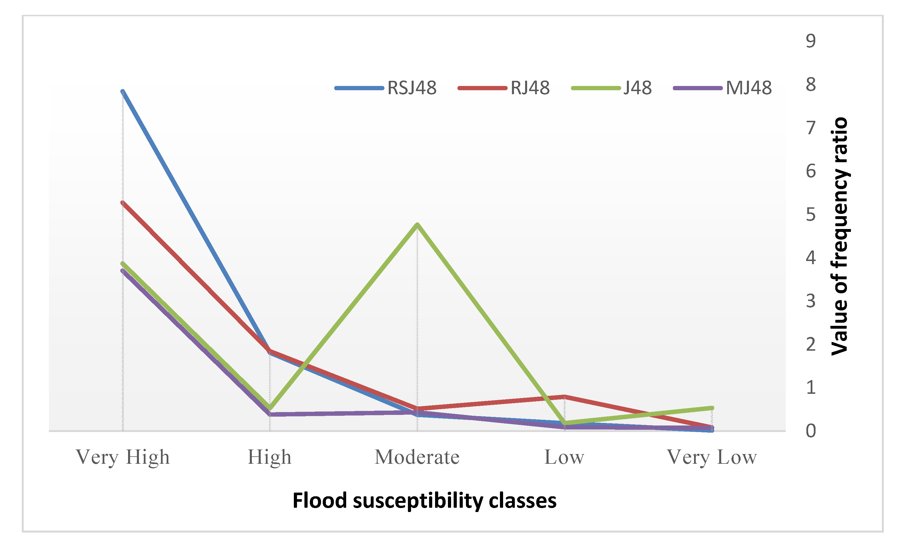
| Flood Susceptibility Classes | J48 | MJ48 | RJ48 | RSJ48 |
|---|---|---|---|---|
| Very high | 18.67% | 24.60% | 16.23 | 9.21% |
| High | 29.13% | 4.13% | 2.56% | 9.54% |
| Moderate | 0.16% | 5.45% | 1.53% | 20.98% |
| Low | 46.63% | 3.02% | 3.31% | 11.55% |
| Very low | 5.39% | 62.81% | 76.38% | 48.72% |
| Criteria | Validation Dataset | Training Dataset | ||||||
|---|---|---|---|---|---|---|---|---|
| J48 | MJ48 | RJ48 | RSJ48 | J48 | MJ48 | RJ48 | RSJ48 | |
| TN | 100 | 95 | 90 | 101 | 221 | 206 | 217 | 221 |
| FP | 15 | 9 | 4 | 9 | 40 | 23 | 28 | 31 |
| FN | 18 | 23 | 28 | 17 | 46 | 61 | 50 | 46 |
| TP | 103 | 109 | 114 | 109 | 227 | 244 | 239 | 236 |
| TPR | 0.85 | 0.83 | 0.80 | 0.87 | 0.83 | 0.80 | 0.83 | 0.84 |
| FPR | 0.13 | 0.09 | 0.04 | 0.08 | 0.15 | 0.10 | 0.11 | 0.12 |
| Efficiency | 0.86 | 0.86 | 0.86 | 0.89 | 0.84 | 0.84 | 0.85 | 0.86 |
| TSS | 0.72 | 0.74 | 0.76 | 0.78 | 0.68 | 0.70 | 0.71 | 0.71 |
| Sensitivity | 0.85 | 0.83 | 0.80 | 0.87 | 0.83 | 0.80 | 0.83 | 0.84 |
| RMSE | 0.33 | 0.35 | 0.39 | 0.3 | 0.35 | 0.4 | 0.34 | 0.33 |
| AUC | 0.871 | 0.929 | 0.893 | 0.951 | 0.850 | 0.889 | 0.906 | 0.931 |
| Models Factors | J48 | RJ48 | RSJ48 | MJ48 |
|---|---|---|---|---|
| Elevation | 18.5 | 16.5 | 21 | 16.5 |
| Distance to stream | 14.4 | 13.4 | 16.9 | 13.4 |
| NDVI | 11.5 | 9.5 | 13.25 | 9.5 |
| Slope | 8.5 | 7.5 | 10.25 | 7.5 |
| LU/LC | 7.5 | 5.5 | 8.25 | 5.5 |
| Rainfall | 5.5 | 4.75 | 7.75 | 4.75 |
| TWI | 3.75 | 3 | 4.5 | 3 |
| SPI | 3.2 | 2.45 | 3.95 | 2.45 |
| Drainage density | 2.7 | 1.95 | 4.2 | 1.95 |
| TPI | 2.25 | 1.5 | 3.75 | 1.5 |
| Lithology | 1.75 | 1.25 | 3.5 | 1.25 |
| Plan curvature | 1.45 | 0.7 | 3.25 | 0.7 |
| Convergence index | 0.75 | 0.5 | 2.25 | 0.5 |
| Soil type | 0.5 | 0.25 | 1.5 | 0.25 |
Publisher’s Note: MDPI stays neutral with regard to jurisdictional claims in published maps and institutional affiliations. |
© 2020 by the authors. Licensee MDPI, Basel, Switzerland. This article is an open access article distributed under the terms and conditions of the Creative Commons Attribution (CC BY) license (http://creativecommons.org/licenses/by/4.0/).
Share and Cite
Arabameri, A.; Saha, S.; Mukherjee, K.; Blaschke, T.; Chen, W.; Ngo, P.T.T.; Band, S.S. Modeling Spatial Flood using Novel Ensemble Artificial Intelligence Approaches in Northern Iran. Remote Sens. 2020, 12, 3423. https://doi.org/10.3390/rs12203423
Arabameri A, Saha S, Mukherjee K, Blaschke T, Chen W, Ngo PTT, Band SS. Modeling Spatial Flood using Novel Ensemble Artificial Intelligence Approaches in Northern Iran. Remote Sensing. 2020; 12(20):3423. https://doi.org/10.3390/rs12203423
Chicago/Turabian StyleArabameri, Alireza, Sunil Saha, Kaustuv Mukherjee, Thomas Blaschke, Wei Chen, Phuong Thao Thi Ngo, and Shahab S. Band. 2020. "Modeling Spatial Flood using Novel Ensemble Artificial Intelligence Approaches in Northern Iran" Remote Sensing 12, no. 20: 3423. https://doi.org/10.3390/rs12203423
APA StyleArabameri, A., Saha, S., Mukherjee, K., Blaschke, T., Chen, W., Ngo, P. T. T., & Band, S. S. (2020). Modeling Spatial Flood using Novel Ensemble Artificial Intelligence Approaches in Northern Iran. Remote Sensing, 12(20), 3423. https://doi.org/10.3390/rs12203423