Article

Weather-Dependent Nonlinear Microwave Behavior of Seasonal High-Elevation Snowpacks

Department of Civil and Environmental Engineering, Duke University, Durham, NC 27708, USA
*
Author to whom correspondence should be addressed.
Remote Sens. 2020, 12(20), 3422; https://doi.org/10.3390/rs12203422
Submission received: 21 August 2020 / Revised: 13 October 2020 / Accepted: 15 October 2020 / Published: 18 October 2020
(This article belongs to the Section Remote Sensing in Geology, Geomorphology and Hydrology)

Abstract

:
Ensemble predictions of the seasonal snowpack over the Grand Mesa, CO (~300 km2) for the hydrologic year 2016–2017 were conducted using a multilayer snow hydrology model. Snowpack ensembles were driven by gridded atmospheric reanalysis and evaluated against SnowEx’17 measurements. The multi-frequency microwave brightness temperatures and backscattering behavior of the snowpack (separate from soil and vegetation contributions) show that at sub-daily time-scales, the ensemble standard deviation (i.e., weather variability at 3 × 3 km2) is < 3 dB for dry snow, and increases to 8–10 dB at mid-day when there is surficial melt that also explains the wide ensemble range (~20 dB). The linear relationship of the ensemble mean backscatter with SWE (R2 > 0.95) depends on weather conditions (e.g., 5–6 cm/dB/month in January; 2–2.5 cm/dB/month in late February as melt-refreeze cycles modify the microphysics in the top 50 cm of the snowpack). The nonlinear evolution of ensemble snowpack physics translates into seasonal hysteresis in the mesoscale microwave behavior. The backscatter hysteretic offsets between accumulation and melt regimes are robust in the L- and C-bands and collapse for wet, shallow snow at Ku-band. The emissions behave as a limit-cycles with weak sensitivity in the accumulation regime, and hysteretic behavior during melt that is different for deep (winter-spring transition) and shallow snow (spring-summer), and offsets that increase with frequency. These findings suggest potential for multi-frequency active-passive remote-sensing of high-elevation SWE conditional on snowpack regime, particularly suited for data-assimilation using coupled snow hydrology-microwave models extended to include snow-soil and snow-vegetation interactions.

Graphical Abstract

1. Introduction

Snow plays an essential role in governing the surface energy and water budgets at high elevations, over large regions of the world at high-latitudes, and at mid-latitudes depending on the time of the year. Monthly mean snow cover varies from 7% to 40% over the Northern Hemisphere [1], and changes in snow cover due to interannual variability and increasing surface air temperatures affect not only regional atmospheric conditions but also large-scale circulation systems, including the global monsoons [2,3,4,5]. The water mass stored in seasonal snowpacks can be estimated from the snow-covered area, snow depth, and snow water equivalent (SWE) metrics. In cold regions and high mountains, winter snowpacks temporarily store freshwater that is subsequently released during melting and thus modulate the availability of water resources [6,7]. The large spatial variability of precipitation, clouds, winds, land-cover, and topography translates into large spatial variability in snow accumulation patterns (snow depth and SWE) and snowpack microphysical properties. Temperature, grain size, and material composition (ice, liquid water content, and particles such as dust or pollution) determine local snowpack surface radiative properties, including emissivity and backscattering behavior, that are spatially organized by topography and land-cover at the meso- and regional scales [8,9].
Remote sensing has long been the primary strategy for large-scale monitoring of snow because of the challenges of access to high remote mountain areas and cold regions [10,11,12]. Since the 1970s, passive microwave satellite observations have been widely used to map areal snow cover and estimate snow depth and SWE. Hall et al. [13,14] lead the first studies to establish the proposition of passive microwave remote sensing of snow that became possible with the launch of microwave radiometers onboard Nimbus 5–6–7 satellites. Rango et al. [15] identified a linear regression equation between microwave brightness temperature (18 GHz and 37 GHz, H- polarization) and snow depth. They demonstrated how the rapid increase of brightness temperatures in the spring could be a robust indicator of liquid water presence and the melting regime’s onset. Chang et al. [16] followed [15] to produce SWE maps over the Northern Hemisphere based on dual-polarization brightness temperature measurements from the Scanning Multichannel Microwave Radiometer (SMMR). Subsequently, Grody and Basist [17] used measurements from the next generation radiometer, the Special Sensor Microwave Imager (SSM/I), to map global snow cover. The relationship between SWE and SSM/I brightness temperatures over 16 land-cover categories was examined by Tait [18], who reported that SWE could be estimated with 95% confidence in smooth non-forested topography. Nevertheless, the retrieval of snow states and properties from passive microwave sensors has long been handicapped by coarse spatial resolution (e.g., 25 × 25 km2 for the Advanced Microwave Scanning Radiometer-Earth Observing System, AMSR-E) that cannot capture the spatial heterogeneity of the snowpack. This results in substantial random and systematic errors in complex topography and in the presence of heterogeneous vegetation, in particular forests that emit more microwave radiation than snow [19,20,21]. Increased absorption and decreased volume scattering in wet snowpacks (> 0.1% snow wetness), and especially in the top layers, result in loss of sensitivity with nonlinear interactions among absorption, surface scattering, and volume scattering [22,23]. Even in barren flat terrain, thermodynamically driven snow microphysics strongly affect brightness temperatures due to high sensitivity to the size of dry snow crystals that vary with time and snowpack history, and thus snowpack stratigraphy [24,25]. Wet snowpacks are more challenging as increases in liquid water content exhibit ambiguous (i.e., noisy) brightness temperature behavior in the warm season after the onset of snowmelt processes. Pulliainen et al. [26] addressed these challenges in part by merging optimally satellite-based brightness temperatures with ground-based observations. They created multi-decadal snow products to monitor the inter-annual variability in snow water resources, albeit at relatively coarse spatial (25 × 25 km2) and temporal (monthly) resolutions, in smooth topography. High spatial resolution (10’s m) radar backscatter measurements at intermediate wavelengths (e.g., Sentinel-1 C-Band) appear to show little sensitivity to dry snow accumulation and high sensitivity to surface roughness and microphysics. The interpretation of the latter can be further complicated by successive cycles of daytime melt and nocturnal refreeze [9] and weather variations, including the spatial organization of diurnal winds [26].
Snow hydrology models driven by near-surface atmospheric forcing provide an alternative to estimate snowpack mass and condition through accumulation and melt processes at sub-daily time-scales in mountainous areas. However, imperfect model physics and numerical approximations [24], uncertainties in meteorological forcing, land-cover and surface heterogeneities, and initial and boundary conditions can significantly impact simulations [27]. Furthermore, the representation of spatial variability tied to topography, wind redistribution, and land-cover among other drivers of snowpack heterogeneity often depend on the model resolution as well and thus are bound to scale [28]. These uncertainties can be addressed in part via data assimilation of remote-sensing observations to guide model physics by constraining model states that effectively amounts to physically-based retrieval [25,29,30,31,32,33]. Operational (i.e., systematic, uncalibrated) robust data-assimilation requires realistic characterization of independent and correlated errors in the coupled snow-hydrology and radiative transfer model as well as observational errors. Data-assimilation can leverage ground-observations for areal cross-validation (e.g., runoff) and for constraining the model at local and regional scales (e.g., snow depth). However, these are not generally available in the remote and inhospitable regions of the world where snow remote sensing is needed. Observational errors have many components, including representativeness, aggregation, and sampling errors. Whereas the characteristics of systematic errors can be learned over time, it is challenging to describe non-Gaussian time-varying errors. An alternative approach to quantify uncertainty is to map the sensitivity space of snowpack physics toward determining the error bounds associated with hydrological response to variable weather and land-cover (e.g., [34]).
This study aims to elucidate the propagation of spatial uncertainty in atmospheric forcing from snowpack physics to radiometric and scattering behavior for high-elevation snowpacks. Ultimately, the goal is to separate uncertainty in snowpack microwave measurements from space (backscattering coefficient and brightness temperatures) from retrieval ambiguity tied to snowpack condition’s spatial variability. For this purpose, we rely on a multilayer snow hydrology model (hereafter referred to as MSHM) [20,21], driven by atmospheric reanalysis, and coupled to the microwave emission model of layered snowpacks (MEMLS) [35,36]. The study area (Grand Mesa, Colorado) and available data sets are described in Section 2. The architecture of the coupled snow physics-radiative transfer modeling framework (hereafter referred to as MSHM/MEMLS) and the experimental design are summarized in Section 3. Detailed model formulations for both MSHM and MEMLS are provided in Appendix A and Appendix B, respectively. Section 4 presents the results focusing on seasonal snowpack hydrology (Section 4.1) and microwave behavior (Section 4.2). Discussion and conclusion are presented in Section 5 and Section 6, respectively.

2. Study Area and Datasets

2.1. Study Area

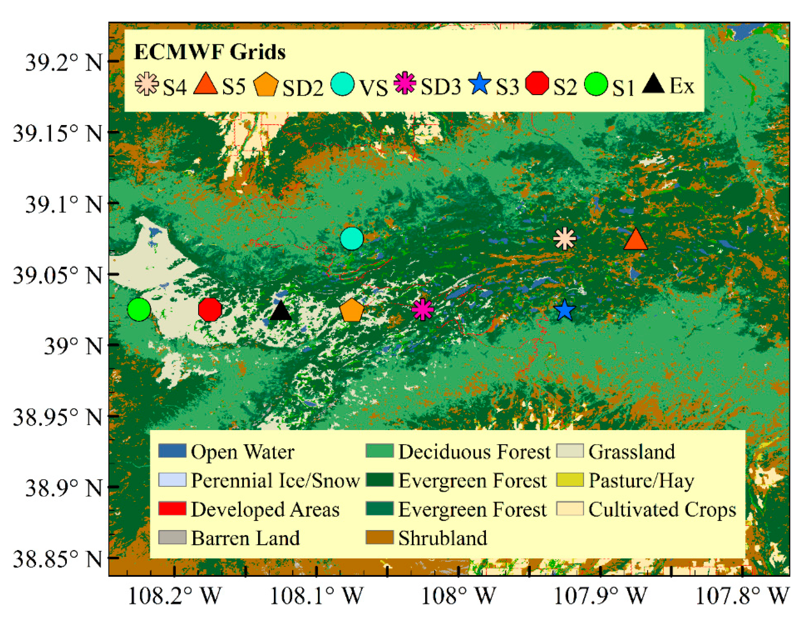
The region of study is Grand Mesa (39° N~39.1° N, 108.2° W~107.8° W), the largest flat-top high mountain in the world (Figure 1). This location is one of NASA’s Snow Experiment (SnowEx) primary field sites [33], where multi-year seasonal intense field measurements are ongoing. We rely specifically on data collected during the February 2017 field campaign, hereafter referred to as SnowEx’17. Land-use land-cover (LULC) is highly heterogeneous with over 300 small lakes and ponds, evergreen and deciduous forests, grasslands, and some barren soil and rock outcrops (Figure 2). Model simulations are conducted in the central part of the Grand Mesa, where most SnowEx’17 snowpit measurements are available.

2.2. Atmospheric Forcing

2.2.1. European Center for Medium-Range Weather Forecasts (ECMWF)

The meteorological variables (air temperature, specific humidity, wind speed, rainfall rate, snowfall rate, incoming shortwave radiation, incoming longwave radiation, and surface albedo) utilized to drive the MSHM were obtained from the ECMWF 3-hourly reanalysis data (in UTC) interpolated to 0.05° × 0.05°) spatial resolution (Figure 1, left panel). The original 3-hourly forcing was linearly interpolated to half-hourly time-steps between 1 September 2016 and 30 June 2017, and are available at https://barros-group.cee.duke.edu/data-access.

2.2.2. High-Resolution Rapid Refresh (HRRR)

The Rapid Refresh (RAP) is a version of the Weather Research and Forecasting (WRF) model developed by the NOAA Earth System Research Laboratory (ESRL) Global Systems Division (GSD). This is an hourly updating, cloud-resolving, convection-allowing model run operationally by the National Centers for Environmental Prediction’s Environmental Modeling Center (EMC) with a nominal resolution of 13 km [37]. The model domain covers entire North America with up to 21 forecast lead times. In the spring of 2016, a high-resolution nested version of the RAP called the High-Resolution Rapid Refresh (HRRR) was developed with a 3-km horizontal grid and one-hour update. It can forecast meteorological variables up to 18 h, including air temperature, specific humidity, wind speed, air pressure, rainfall rate, snowfall rate, incoming shortwave radiation, and incoming longwave radiation. Hourly HRRR data (data assimilation and forecast modeling systems), specifically + 01 h forecasts, were obtained from the Center for High-Performance Computing (CHPC) at the University of Utah [38]. Time-series of HRRR meteorological data from 43 grids over the Grand Mesa (Figure 1, right panel) were linearly interpolated to the MSHM time-step (30 min) from 1 September 2016 to 30 June 2017. Numbering and naming conventions and geographical correspondence between ECMWF and HRRR grids are provided in Supplementary Information, specifically Table S1 and Figure S1a,b.

2.3. North American Land Data Assimilation System (NLDAS)

Initial preprocessing showed that the time-varying ECMWF albedo values are inconsistent with observed snow cover conditions over Grand Mesa and independent satellite-based estimates. The broadband surface albedo from the North American Land Data Assimilation System (NLDAS) [39] at ~12.5 × 12.5 km2 spatial resolution was selected because it is available at hourly intervals. Thus, no further interpolation was required to resolve the diurnal cycle. The average of the four NLDAS grids in Grand Mesa was calculated first for the hourly values and subsequently interpolated to half-hourly intervals. The spatial variability is small. Consequently, the same albedo value is specified for all ECMWF and HRRR grids at each time-step.

2.4. SnowEx’17 Field Campaign Data

Data from the NASA SnowEx campaigns can be obtained from (https://nsidc.org/data/snowex). Data relevant for this study include snow depth, SWE, snow density, and temperature profiles [40]. These data are used to evaluate co-located MSHM simulations and characterize the uncertainty associated with sub-grid heterogeneity within ECMWF grid cells and across the Grand Mesa.
Snowpit observations were obtained by digging trenches (destructive and irreversible measurements) for a one-time-only sampling of the density and temperature profiles. Thus, there are no repeats at the same location. It is important to highlight the gap in spatio-temporal scales between the in-situ snowpit data (point scale, near-instantaneous) and the ECMWF and HRRR forcing and MSHM simulations (kms, mins-hours). Tables S2–S4 provides geospatial coordinates of snowpit locations corresponding to ECMWF grid cells S2, SD3, and S5 (Figure 1 and Figure 2) used in this paper to assess MSHM performance.

3. Experimental Design

3.1. MSHM/MEMLS Modeling Framework

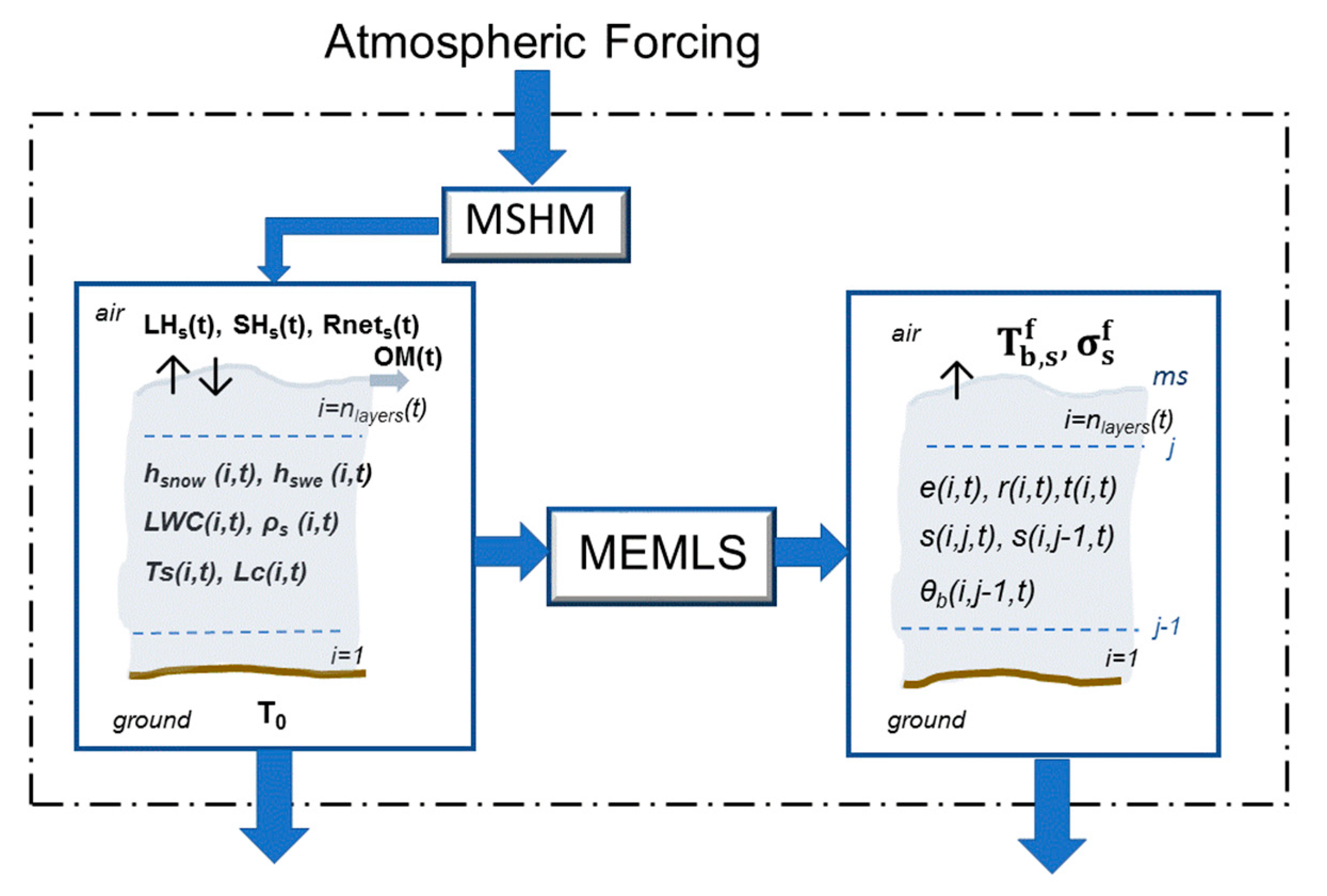
The architecture of the coupled MSHM/MEMLS framework is summarized in Figure 3. The MSHM represents the snowpack as a multilayer column (1D in the vertical, Figure 3 right panel) with layers added (by splitting individual layers) or removed (by combining individual layers) depending on precipitation and compaction rates to meet a minimum water equivalent depth criterion for each layer (0.02 ± 0.01cm). Exchanges of mass and energy at the snowpack surface and adjacent layers in the snowpack column (1D) are simulated using centered finite-difference approximations following [41]. The formulae used to describe key model processes are summarized in Appendix A. The flowchart that describes model structure and linkages among model physics components is depicted in Supplementary Figure S2. Additional implementation details and alternative parameterizations can be found in [20,21]. The ongoing testing and implementation of the MSHM coupled to an existing distributed hydrology model is out of the present work scope. Therefore, snowpack surface conditioning (surface roughness and transient morphology), snow erosion and redistribution by winds, and the structural effects of forest cover on snow hydrology on the one hand and microwave behavior on the other are not considered in the version of the MSHM/MEMLS used here. These effects are accounted for only in the time-varying values of albedo specified and in the atmospheric forcing (specifically, low-level winds, air temperature, and relative humidity) to the extent that land-cover is parameterized in the underlying numerical weather prediction model.
The MEMLS model was developed based on the six-flux theory to simulate multiple volume scattering and absorption (Figure 3, right panel), including radiation trapping from internal and coherent reflections at layer interfaces (see Figures S3 and S4). It was first implemented to simulate multi-frequency microwave brightness temperatures [36] with good performance compared to satellite data [20,21], and it has been further enhanced to simulate backscattering [35]. Implicit in the MSHM/MSML coupling is the shared spatial resolution determined by the atmospheric forcing’s spatial scale and the assumption that the subgrid-scale variability in snowpack states (e.g., snow types), and consequently in microwave emissions and backscatter, can be neglected [23,26]. The coupled MSHM/MEMLS modeling framework is run continuously for predictive purposes from September (9/1/2016) through June (6/30/2017) at half-hourly time-steps driven by independent meteorological forcing (ECMWF, HRRR). SnowEx’17 snowpit measurements during February 2017 are used for evaluating MSHM predictability of snowpack physical properties and snow hydrologic states. The density of fresh snow is specified as 30 kg/m3.

3.2. Ensemble Design

The impact of uncertainty tied to meteorological forcing’s spatial variability on the simulated snowpack’s physics and microwave behavior is investigated using ensemble forecasts (EF). Two ensemble families were designed. Members of the first ensemble family (EFF1, 3 km resolution) are obtained by replacing ECMWF forcing with HRRR “perturbations,” neglecting spatial resolution differences between ECMWF and HRRR. EFF1 consists of 6 different ensembles (0–5), each corresponding to varying combinations of ECMWF and HRRR forcing as summarized in Table 1 for a total of 1978 (= 387 × 5 + 43) simulations (9 ECMWF grids × 43 HRRR perturbations = 387 members each for Ensemble 0–4, and 43 members for Ensemble 5). Members of the second ensemble family (EFF2, 750 m resolution) are obtained by replacing HRRR precipitation analysis at the native 3 km resolution with 16 precipitation replicates obtained by fractal downscaling of the HRRR precipitation fields [42,43,44,45]. For reference, the cumulative snowfall and rainfall curves and the concurrent time-series of near-surface air temperature (2 m) from the HRRR analysis are provided in Figure S5. EFF2 consists of 9 ensembles for each of the HRRR grids nearest to nine ECMWF reference grids centers with 16 members for a total of 144 simulations. Figure S6 illustrates the downscaling strategy graphically. The fractally downscaled precipitation at 750 m resolution is the ensemble mean of fifty rainfall fields generated recursively [43,45]. Whereas it is possible to downscale the precipitation to higher spatial resolution, recent work [9] suggests robust interpretable scaling behavior in SAR measurements at C- and L-bands at spatial scales in the 400–1000 m range.
The EFF1 ensemble spread expresses the forcing uncertainty at 3 km resolution over the relatively large Grand Mesa domain (Figure 1). In contrast, ensemble differences among each of the nine ECMWF reference grids reflect differences in land-cover and land-form that impact surface roughness, friction velocity, and surface winds. The EFF2 ensemble spread stems from increased spatial variability of precipitation from 3 km (HRRR pixel) to 750 m (downscaled precipitation) and aims to capture the uncertainty tied to precipitation’s stochastic redistribution at HRRR sub-grid scales.

4. Results

To characterize uncertainty in snowpack microwave behavior (backscattering coefficient and brightness temperatures) tied to snowpack states conditional on regional weather, we view the coupled snow hydrology-radiative transfer model as an instrument simulator. Therefore, a key challenge is that the snow hydrology model must represent the governing physical processes and capture the fundamental drivers of radiative properties change in the snowpack. Thus, we start by evaluating the model’s capability to capture snow hydrologic processes and quantifying the range of uncertainty in snowpack hydrologic properties associated with meteorological forcing in Section 4.1. The active and passive microwave behavior of the snowpack is examined in Section 4.2. Analysis of model results and discussion is centered on ECMWF grid cells S2, SD3, and S5 (Figure 1) to capture the snowpack’s evolution in the western, central, and eastern sub-regions of Grand Mesa, respectively. Each of these three grids is collocated with HRRR grids and contains several snowpit observations obtained during SnowEx’17 (snowpit geo-coordinates and acquisition dates and times are provided in Tables S2–S4).

4.1. Snowpack Hydrology

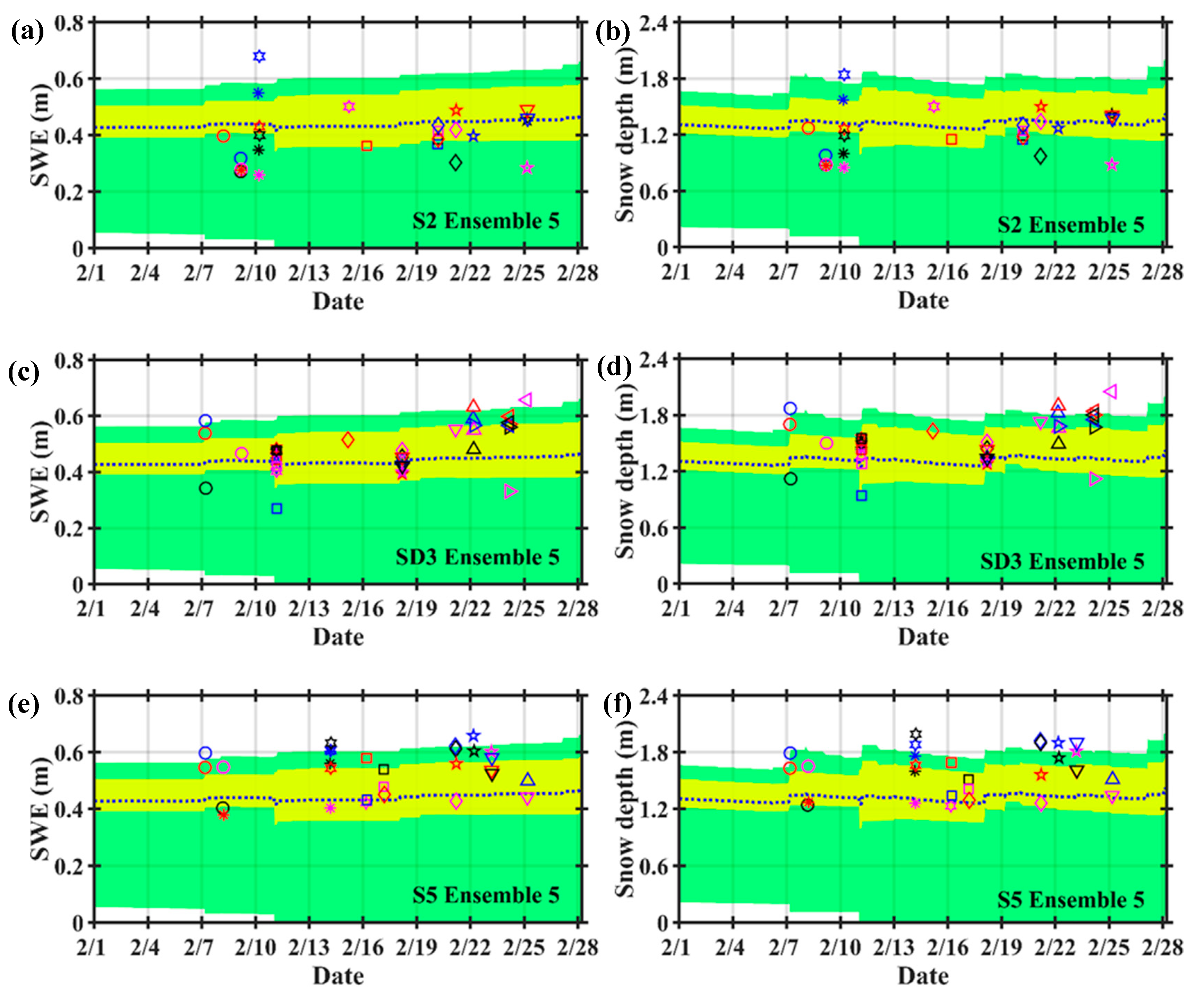
SWE and snow depth—SWE and snow depth predictions begin on 9/1/2016 and last until 6/30/2017 for each EFF1 ensemble to capture the snowpack’s full seasonal evolution in Grand Mesa, as shown in Figure S7. The severe snowfall underestimation in the ECMWF forcing is apparent in the Ensemble 0 and Ensemble 1 results amounting to 100% and 300% differences respectively for SWE and snow depth concerning Ensemble 2 and Ensemble 5. These differences amount to about 400 mm in SWE at the end of the accumulation season, which is about four-fold the Northern Hemisphere bias identified by [46]. This is illustrative of the challenges of modeling orographic precipitation. The contrast in the spread of the yellow (25th and 75th percentiles) and green (max and min) envelopes between Ensembles 0 and 1 demonstrates the impact of the space-time variability of near-surface air temperature in driving heterogeneity among ensemble members. Solid and liquid precipitation is not explicitly differentiated. Standard approaches, such as using near-surface air temperature below a certain threshold (e.g., 273.15 K) to identify snowfall, do not work well because of the ECMWF near-surface air temperature exhibits strong warm bias as compared to observations and HRRR values as well. Indeed, excessive early warming leads to the dramatic melting and snowpack retirement almost two weeks earlier in Ensemble 1. Dramatic improvement is achieved when the HRRR precipitation forcing is introduced in Ensemble 2. There are no significant differences in snow mass accumulation and melt patterns among Ensembles 3 and 4 (not shown) and Ensemble 5. This result indicates that precipitation and air temperature, particularly snowfall, are the critical local meteorological forcing necessary to capture the seasonal snowpack over Grand Mesa as long as radiative forcing and winds are representative of regional conditions. This result is expected and consistent with [27], who found that the sensitivity of a snow hydrology model to forcing was dominated by precipitation bias errors.
SnowEx’17 snowpit measurements at S2, SD3, and S5 are used to evaluate the MSHM Ensemble 5 evolution of SWE (Figure 4a,c,e) and snow depth (Figure 4b,d,f). For reference, the cumulative predicted snow mass (SWE) in February 2017 at the ECMWF grid cell scale (~5 × 5 km2) does not reach the highest measured value across the Grand Mesa. This is attributed in part to HRRR underestimation of precipitation, especially snowfall, and uncertainty in the snowpit measurements themselves. The scale gap between point measurements (the individual snowpits) and Ensemble 5 members representing areal averages at the HRRR grid cell scale (3 × 3 km2) is a significant source of uncertainty and ambiguity in interpreting results. One additional source of snow depth uncertainty is snowpack compaction’s empirical parameterization in the model (Appendix A, Appendix A.1). Specifically, the terms corresponding to overburden effects exhibit high sensitivity to snow accumulation and, therefore, propagate snowfall uncertainty to snow depth nonlinearly.
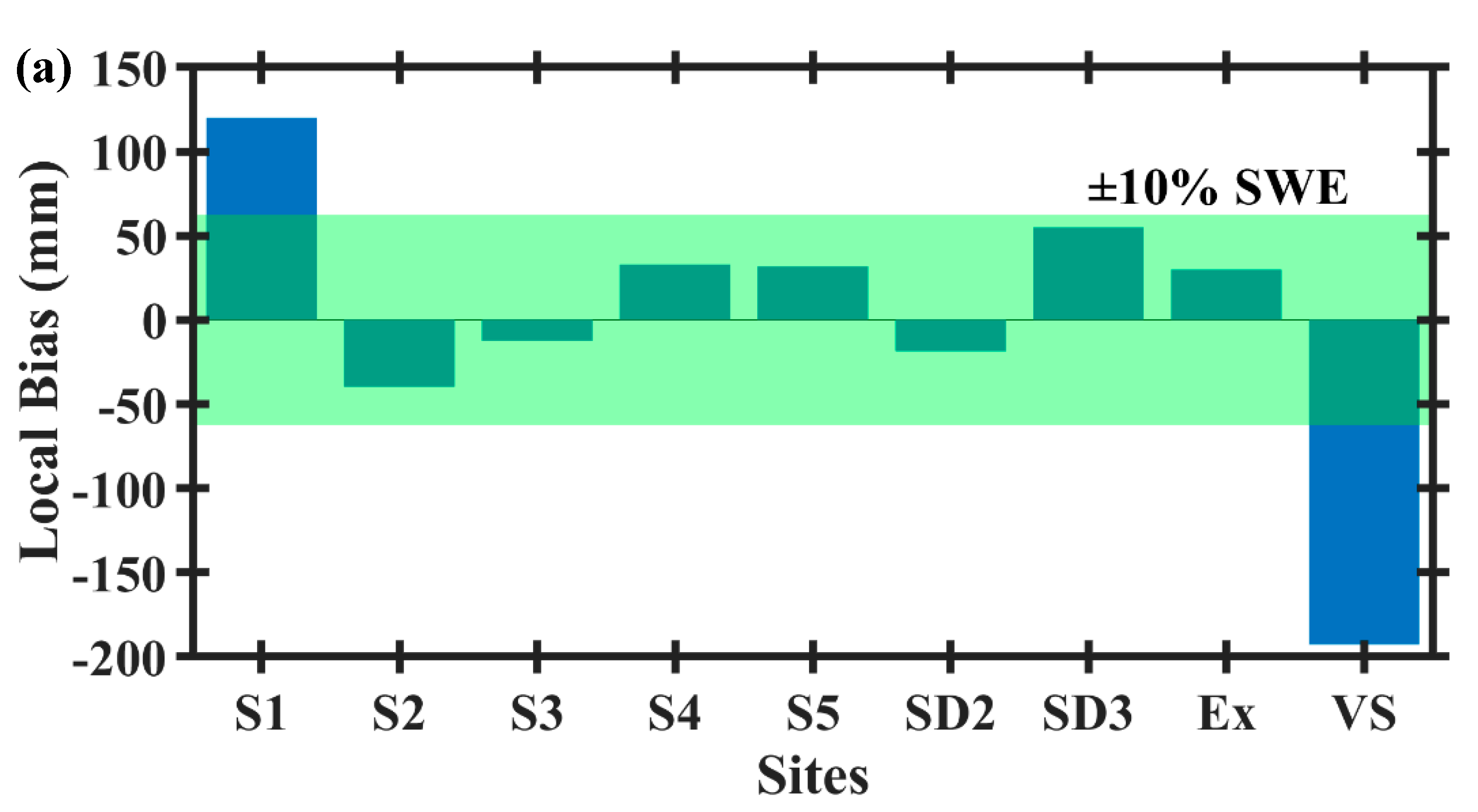
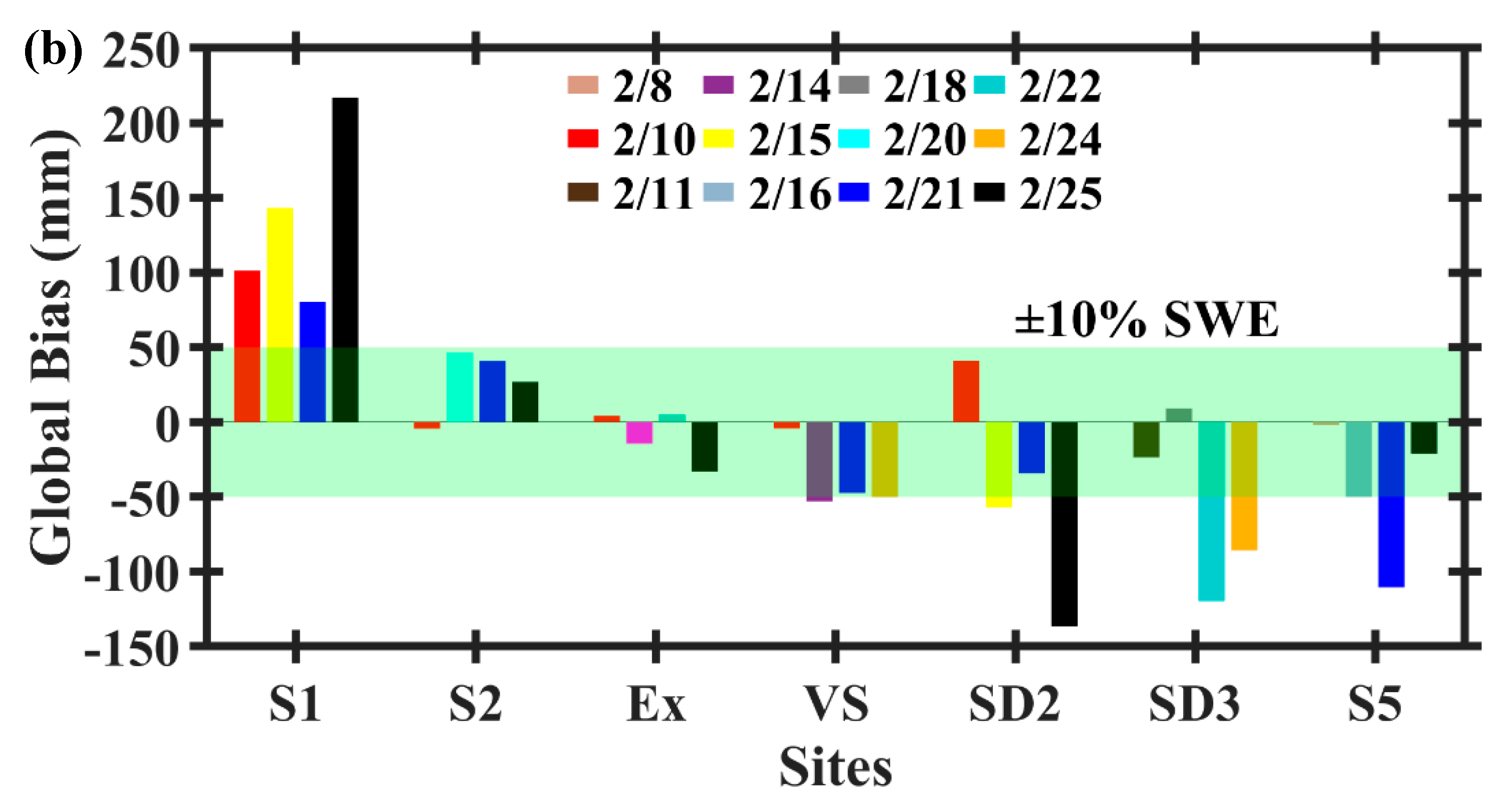
The model results during SnowEx’17 were organized further in two sets for evaluation against the snowpit measurements according to spatial scale: (a) local–Ensemble 5 predictions for the member that is nearest to the center of each reference ECMWF grid (Table S1), and (b) global–Ensemble 5 mean across the Grand Mesa. Figure 5 shows the local (top row) and global (bottom row) model bias during February 2017. Inspection of the local bias (local Ensemble 5 member–snowpit average within the corresponding ECMWF grid cell) shows that SWE estimates are within ±10% of the snowpit measurements except at S1 and VS. This indicates that given the HRRR snowfall estimates the snowpack mass and energy budgets are well simulated without the need for calibration or special processing of the data. The sizeable accumulation biases at S1 (positive bias, surplus) and VS (negative bias, deficit) are attributed to uncertainty in wind effects. Sources of uncertainty in near-surface wind magnitudes include the fact that HRRR near-surface winds are used directly in the simulations without downscaling from HRRR resolved scales (4–6 Δx = 12–18 km) to the grid point scale (3 km), which introduces biases in the surface friction velocity [47], lack of topographic corrections to account for the steep slopes at S1 in the western edge of the Mesa, and corrections to account for structured roughness due to the presence of forest at S5. Additionally, as mentioned earlier, the MSHM implementation used here does not simulate wind-redistribution. This explanation is supported further by the temporal variability of the global bias (Ensemble 5 mean-snowpit average within the reference ECMWF grid cell) and by the west-east differences with a larger negative bias to the east (e.g., SD2, SD3, and S5) in the more forested areas of the Grand Mesa where snow accumulates in the second half of February (see Figure 2) and positive bias to the west (e.g., S1).
Snow Stratigraphy—The temporal evolution of snow density and temperature profiles at S2 corresponding to Member 8 of Ensembles 1, 2, and 5 are shown in Figure S8. The average of co-located snowpit profiles is superimposed on simulated profiles for the available dates. As expected, Ensemble 5 members are the most realistic in that the simulated snow depths are close to the measurements. There is, however, no significant difference in the temperature gradients in the upper half of the simulated snowpack among members of Ensembles 2 and 5, demonstrating the governing role of the near-surface air temperature in the turbulent heat exchange at the air-snow interface. The differences between model and snowpit average density are generally less than 50 kg/m3 at the same depth, which is adequate for coupled forward modeling of snow hydrology and radiative transfer using MEMLS [20,21,22,34].
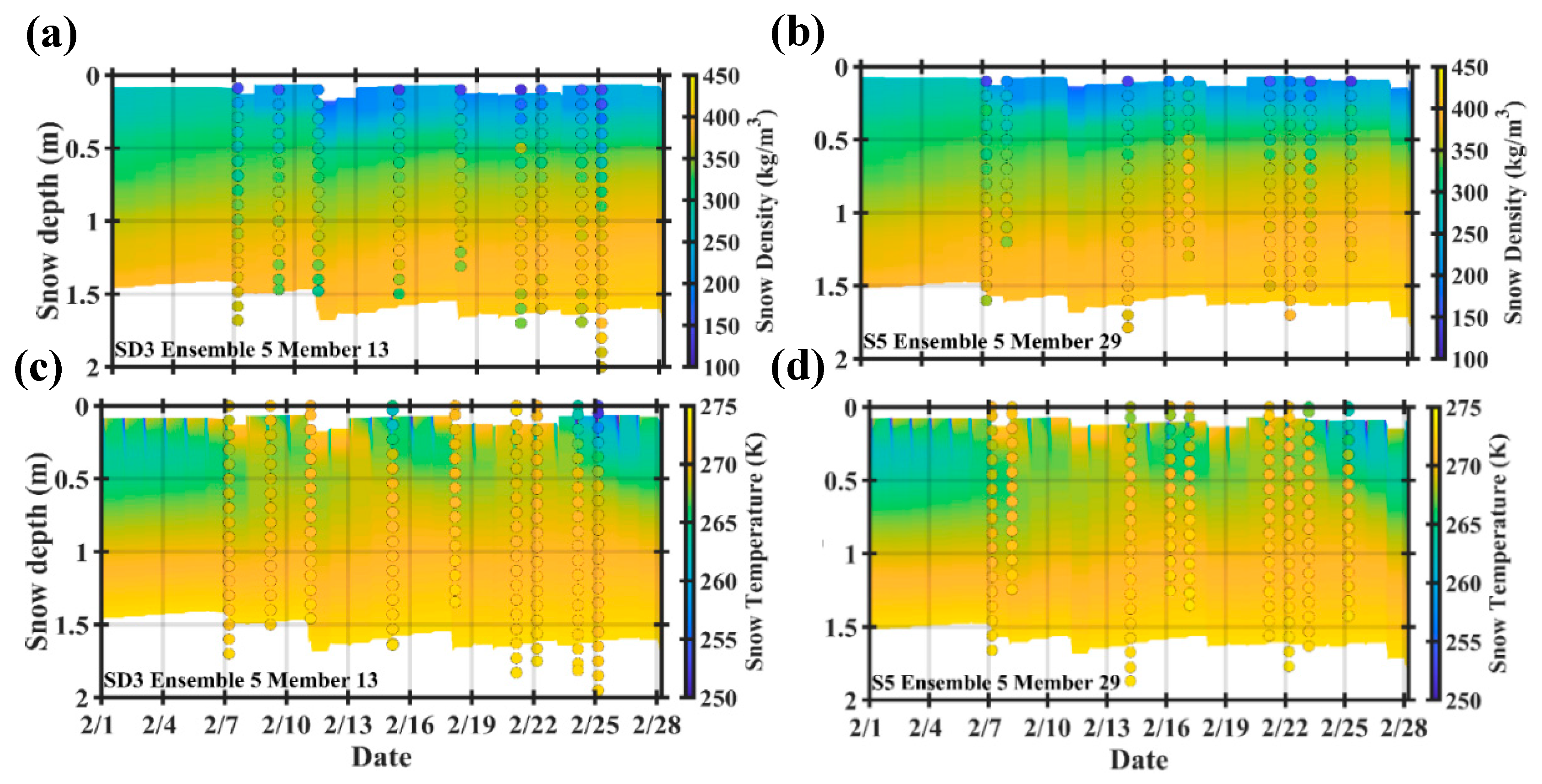
Temperature and density profiles at SD3 (Member 13) and S5 (Member 29) for Ensemble 5 only are shown in Figure 6. Ensemble 5 model predictions capture well the isothermal behavior of the snowpack at the three sites (bottom row in Figure S8 for S2, and Figure 6 for SD3 and S5) as well as the signature of significant snowfall and cold weather events. The temporal evolutions of the number of snowpack layers and top layer depth simulated for the three reference grids are shown in Figure S9. SnowEx’17 measurements of top-layer snow temperatures are generally close to the freezing point (273.15 K) and nearly isothermal throughout the snowpack except during two cold periods on February 15 and February 25. Daytime temperatures well below the freezing level in the top 20–50 cm for these two events are captured well by the model consistent with the local surface energy budget. For instance, Figure S10 shows the substantial reduction in daytime snowpack sensible heat flux at S2 in the February 22–25 period. Besides, note the short-lived periods of steep decreases in upper snowpack temperature tied to transient reductions in cloudiness that translate into approximately halving of incoming longwave radiation in the February 22–25 period (e.g., Figure S11). The contribution of incoming longwave radiation to the surface energy budget is critical [48]. The reduction of incoming longwave radiation (~150 W/m2) on clear cold days impacts snowpack temperatures at intermediate depths corresponding to the top 50 cm at S2 (Figure S8) and as much ~100 cm for the deeper snowpack at SD3 and S5 (Figure 6) due to faster cooling in less dense snow.
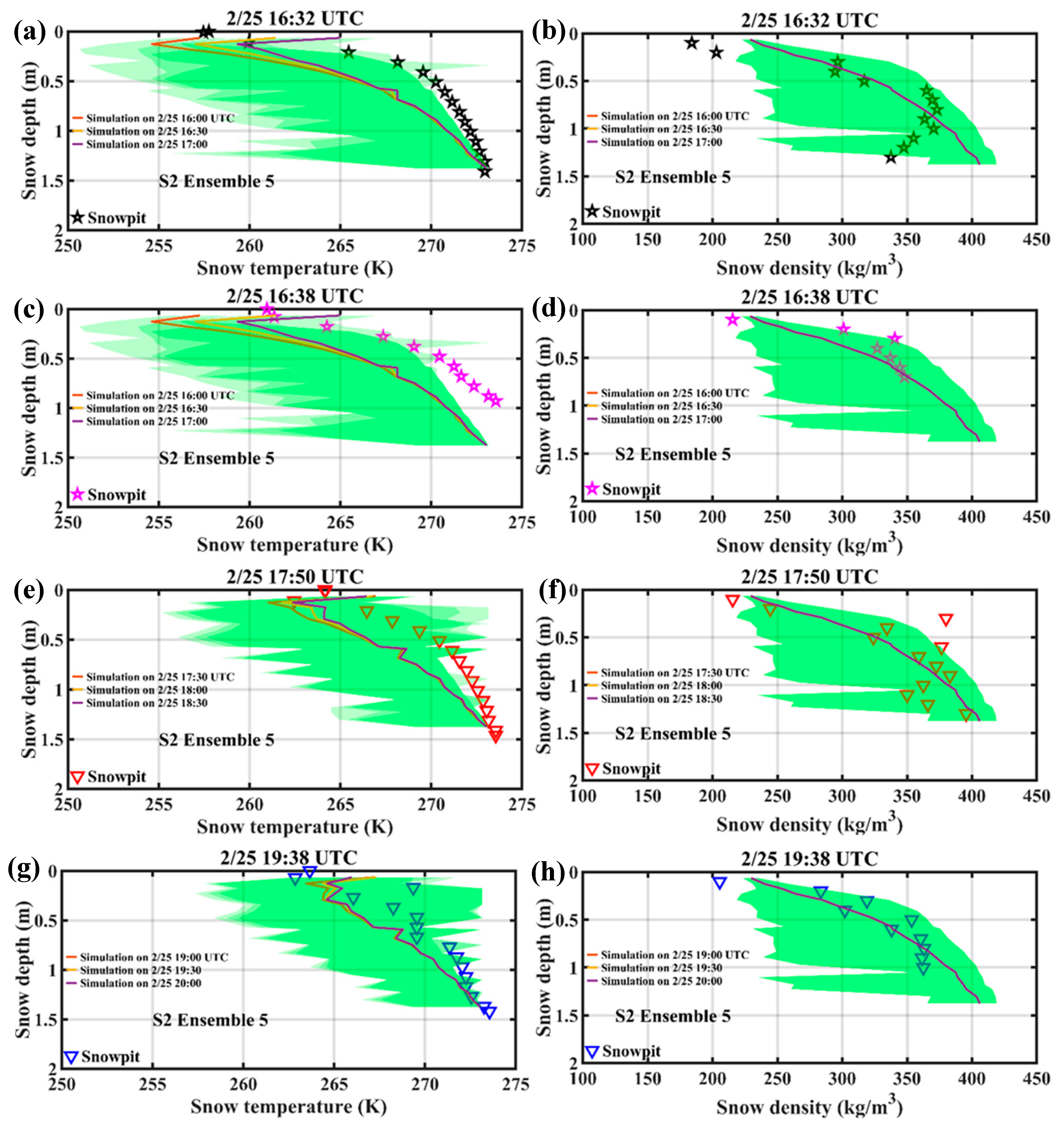
Figure 7 illustrates the behavior of Ensemble 5 against measurements of snow density and snow temperature from each of four snowpits within S2 on February 25. A caveat of daytime snowpit profile measurements is that they are disturbed at least in part due to excavation. The snowpack facies is directly exposed to the environmental air, which can explain at least in part the warmer temperatures in the deeper layers. The goal here is to compare the ensemble spread with the variability of snowpit measurements within S2 that captures snowpack heterogeneity due to space-time variability of meteorological forcing within the Grand Mesa at the small mesoscales of the HRRR analysis (3 × 3 km2), and the snowpit measurements represent subgrid-scale variability. Simulated snow density profiles replicate the measurements closely except at the bottom of the snowpack. The measured density profiles display an “inversion” with lower densities 5–20 cm above the snow-soil interface (e.g., top right in Figure 7). This behavior suggests depth hoar formation at the snow-soil interface that is not explicitly described in the model.
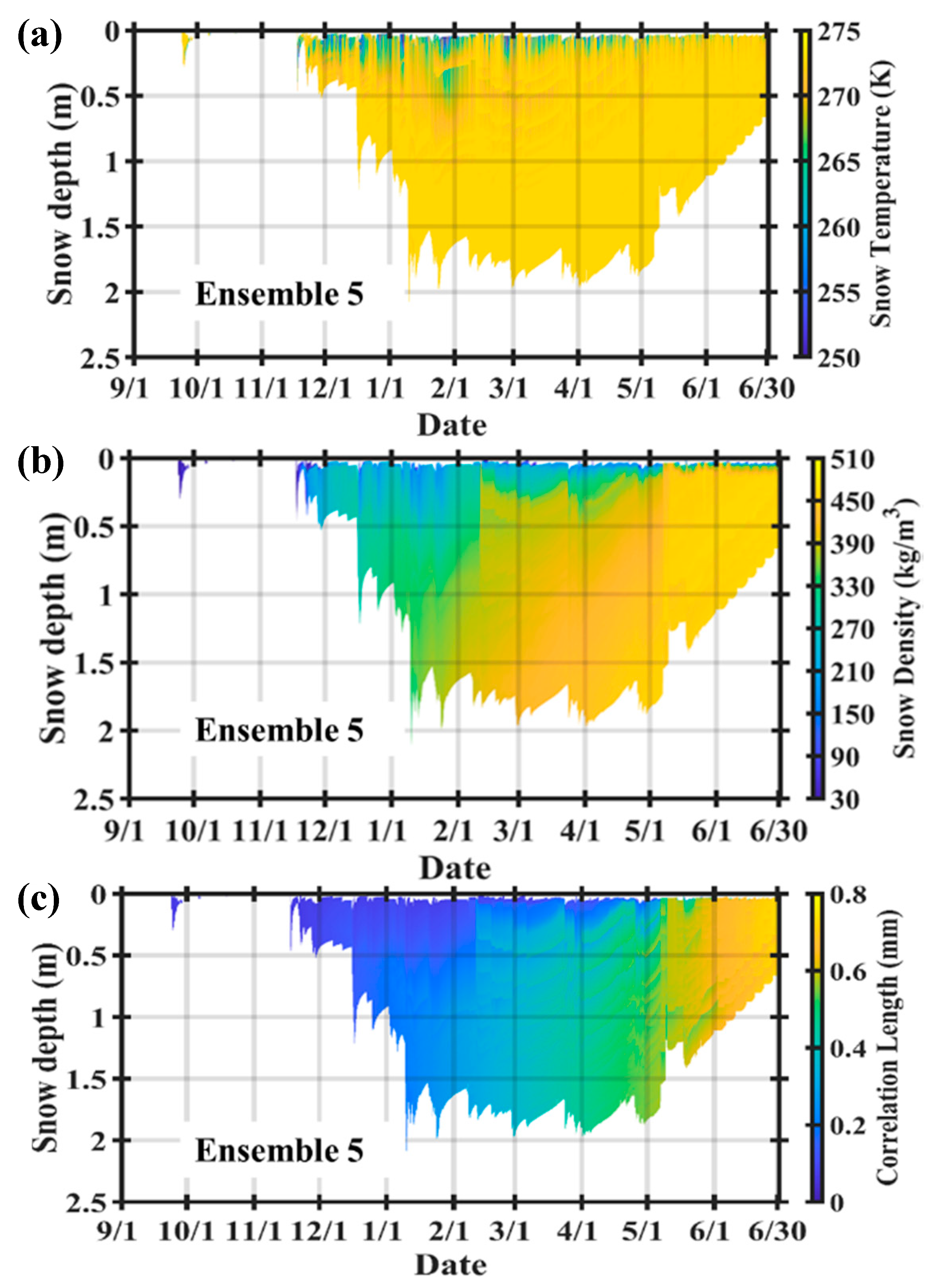
Overall, the MSHM driven by HRRR atmospheric forcing and constrained by the mass and energy balance exhibits behavior consistent with SnowEx’17 snowpit observations across the Grand Mesa. Figure 8 shows the continuous simulation of snowpack temperature, density, and snow correlation length profiles for the 2016–2017 hydrologic year, including accumulation and melt regimes. The model depicts the decreases in density and cold temperatures at the top of the snowpack due to snowfall. The nearly isothermal profiles during warm periods are similar to the snowpit observations. The latter result from surface melt retained in the top layer or that percolates and freezes, as shown in Figure S8. Note the long duration of the snow-on season in 2017 that lasts until the end of June, consistent with Landsat and Sentinel-1 satellite observations [9].
A coordinated inspection of Figure S7 (bottom row, snowpack SWE, and snow depth), Figure S12 (meteorological forcing: precipitation and air temperature), and Figure 8 (snowpack stratigraphy) suggests modest uncertainty in SWE (~±15%) and snow depth (~±10%) during the accumulation regime. At the Grand Mesa scale, uncertainty peaks in the melting season with values up to 50% attributed to weather, and in particular, air temperature. Interestingly, uncertainty in snow density as a function of snow depth (Figure 8b) is more considerable in the fall season and through the warming period in the first half of February (Figure 8a). It collapses as the snowpack ages and becomes deeper during the accumulation season. Large variations in density with fresh snowfall are limited to the top 50 cm. The layering of snow correlation length reveals the vertical structure of snow microphysics (Figure 8c) to be more complicated than suggested by the apparent simplicity of the physical parameterization used in the model [36,49]. This complex stratigraphy is the outcome of the temporal integration of nonlinear interactions among snow aging processes, the diurnal cycle of radiative forcing, and weather systems that affect the snowpack temperature, the occasional fresh snowfall, and rain-on-snow events. Snowpack microphysical and thermodynamic stratigraphy, along with snow mass and surface roughness, govern the snowpack’s effective radiative properties and its emissions and scattering behavior to be discussed next.

4.2. Snowpack Microwave Emissions and Scattering Behavior

The snowpack ensembles generated by the snow hydrology model were used in MEMLS to simulate dual-polarization backscatter coefficients (σ) and brightness temperatures (Tb) at L- (1.3 GHz), C- (5.6 GHz) and Ku- (13.5 GHz) and Ka- (35.7 GHz) bands with parameters summarized in Table 2. Backscatter at the snow-ground interface, which is dominant in dry snow conditions at low frequencies (e.g., L- and C-band), does not change in time during the snow-on season. However, it will vary from location to location, depending on the local substrate (soil type, geology, vegetation cover) and topography [9]. The snow-ground interactions are separated from volume scattering in the multi-layer snowpack by specifying the relevant model parameters and boundary conditions as zero (Table 2). The backscattering behavior examined in this manuscript is strictly attributed to the scattering within the snowpack and at the air-snow interface. The focus is strictly on understanding the microwave behavior of heterogeneous snowpacks that can be generalized. The objective is to examine the propagation of spatial uncertainty associated with meteorological forcing at the Grand Mesa scale in the microwave domain and estimate uncertainty due to sub-grid scale variability of precipitation. Only a selection of results that synthesizes the main findings is shown here. We quantify sensitivity in terms of ensemble standard deviation and range.
Despite the spatial resolution gaps (2–3 orders of magnitude) between available microwave measurements during SnowEx’17 and the simulations (3 km), the model predictions are compared against Sentinel-1 C-band data (30 m) produced by [9] and against ground-based multi-frequency radiometer measurements (0.6 m) in the vicinity of snow pits [50] to assess the coupled model’s ability to capture the spatial variability of microwave behavior across the Grand Mesa based on atmospheric forcing alone. First, the statistics of the Sentinel-1 data aggregated to the spatial resolution of the hydrology model (i.e., from 30 m to 3 km) are contrasted with Ensemble 5 statistics on 7 and 24 February 2017, at the time of overpass (Figure S13). The difference in Sentinel-1 and Ensemble 5 means suggest that, on average, the contribution of snow-ground interactions to the observed backscatter across the Grand Mesa is ~7–8 dB. The variance of the Sentinel-1 data aggregated to the HRRR resolution is larger than that of Ensemble 5. It captures realistic spatial heterogeneity in land-cover and landform; the range behaves in the same way, increasing when there are isolated surficial melting spots on 2/24. The surface-based radiometry (SBR) measurements are effectively point-scale measurements. Thus, concurrence between the SBR and Ensemble 5 is expected to be curtailed by multiscale spatial variability within the HRRR grid, depending on local conditions. The SBR measurements are within the range of Ensemble 5 and close to the ensemble mean on 2/7, consistent with weak spatial variability in atmospheric forcing (Figure S14). On 2/24, the continuous SBR Tb-Vs begin very low and rapidly increase and converge to the range of Ensemble 5 at mid-day when surficial melting is ongoing. Tb-H measurements, however, remain much colder than the Ensemble 5 mean close to the lower bound of the ensemble range. The SBR measurement locations on 2/24 are in the forested area of Grand Mesa (ECMWF reference grid points S4 and S5, Figure 1 and Figure 2). The measured cold Tbs suggest lower H-pol emissivity compared to simulated values at the same frequencies. Lower H-pol emissivity is associated with large grain sizes (and large correlation lengths) and, or crusts that emerge respectively from surface hoar processes (sublimation followed by recrystallization) and due to overnight refreeze of daytime melt [51]. Figure S16 shows that the predicted profiles of snow correlation length are close to the values estimated from measured grain-sizes, although underestimation can occur in the top layer of the snowpack when the temperature gradients are steeper (e.g., Figure S16, top row). These processes are not explicitly addressed in the model snow microphysics currently (Appendix A.7).
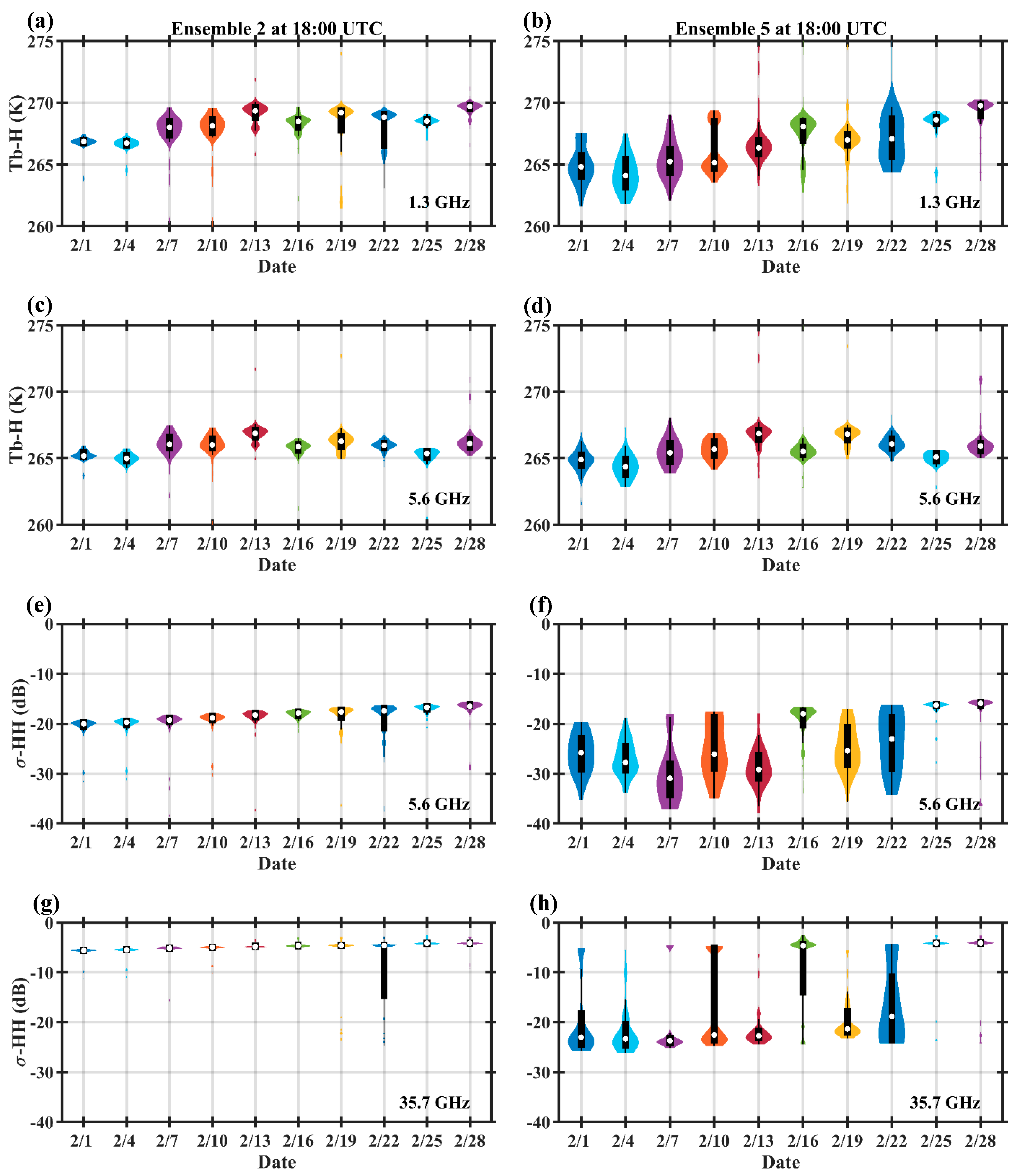
Sensitivity to meteorological forcing—The propagation of uncertainty from the snow hydrology to the microwave radiative transfer model is examined first by contrasting C-band (5.6 GHz) active σ-HH and passive Tb-H and active Ka-band (35.7 GHz) for EFF1 Ensembles 2 and 5 that differ in boundary-layer forcing (wind speed and specific humidity) and incoming radiation (Table 1). Recall that there is a small net change in SWE (<5 cm) during the month of February in Grand Mesa, and the variability on each date reflects mostly the concurrent spatial variability of snowpack radiative properties. The results (Figure 9) for Ensemble 2 exhibit much less variability than Ensemble 5 due to the boundary-layer conditions that modulate the surface energy budget independently of frequency across the Grand Mesa. Backscatter and brightness temperatures exhibit highly nonlinear sensitivity as measured by the standard deviation, respectively ± 10 dB and ± 2 K. This sensitivity is more significant at the longer wavelengths (i.e., 1.3 and 5.6 GHz), albeit the range is near twice as large. Note the collapse of the violin diagrams and thus uncertainty during the cold snap in late February and the higher σ with larger uncertainty for Ka-compared to C-band. For the remainder of this discussion, we will focus on EFF1 Ensemble 5 results.
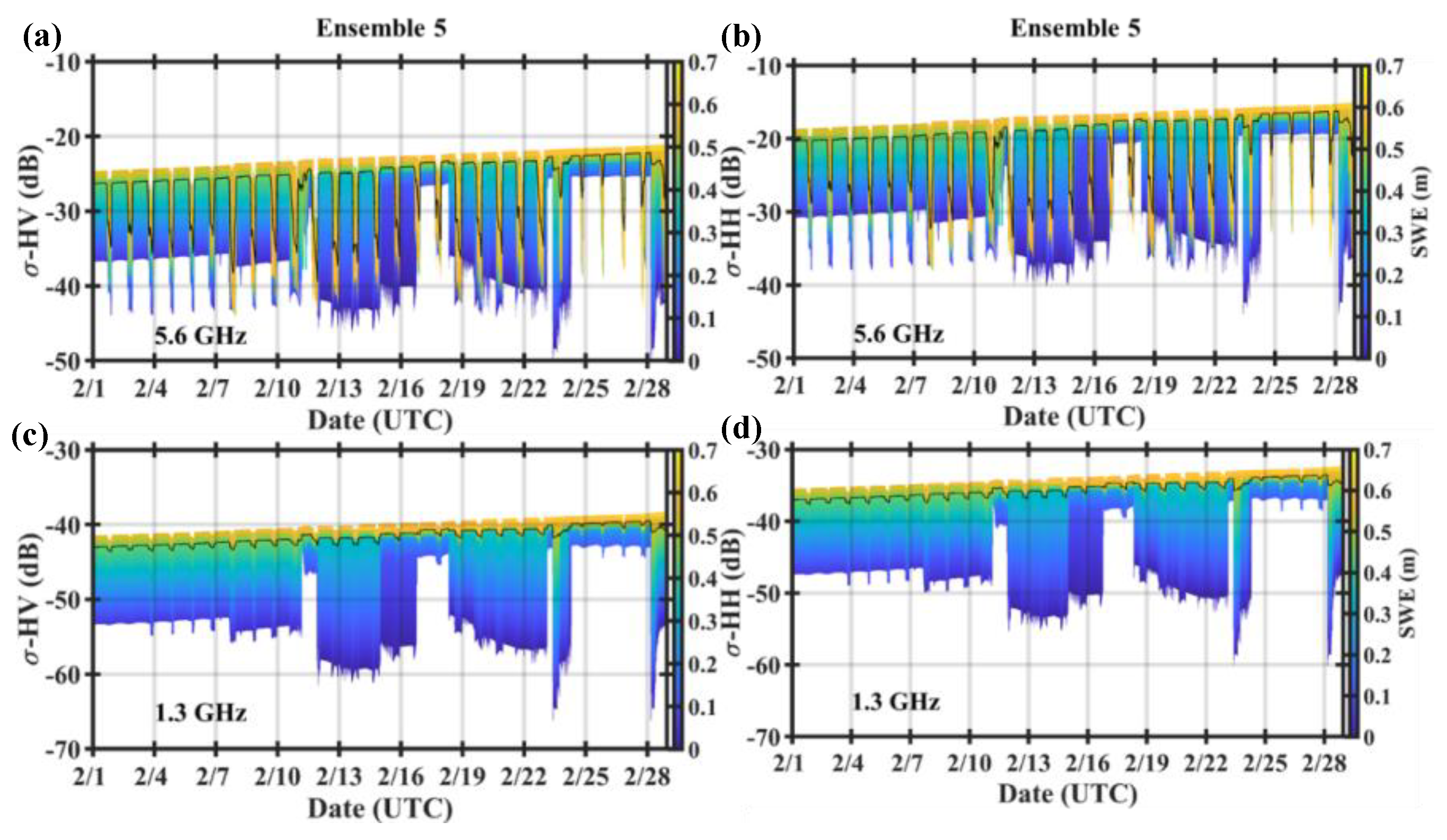
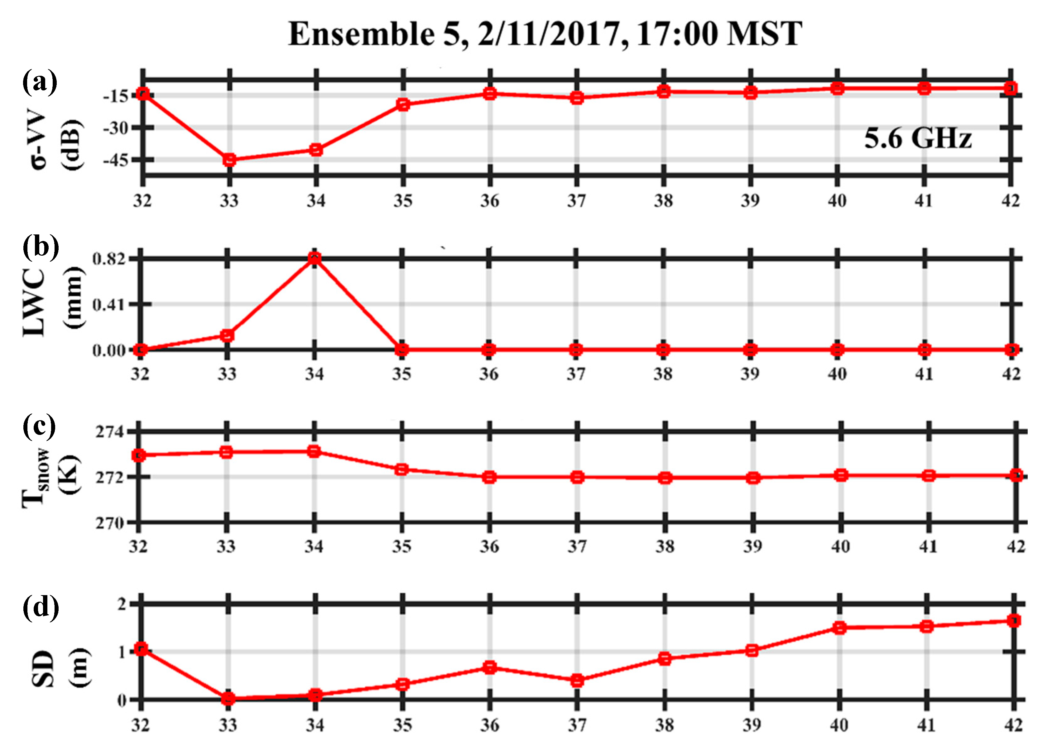
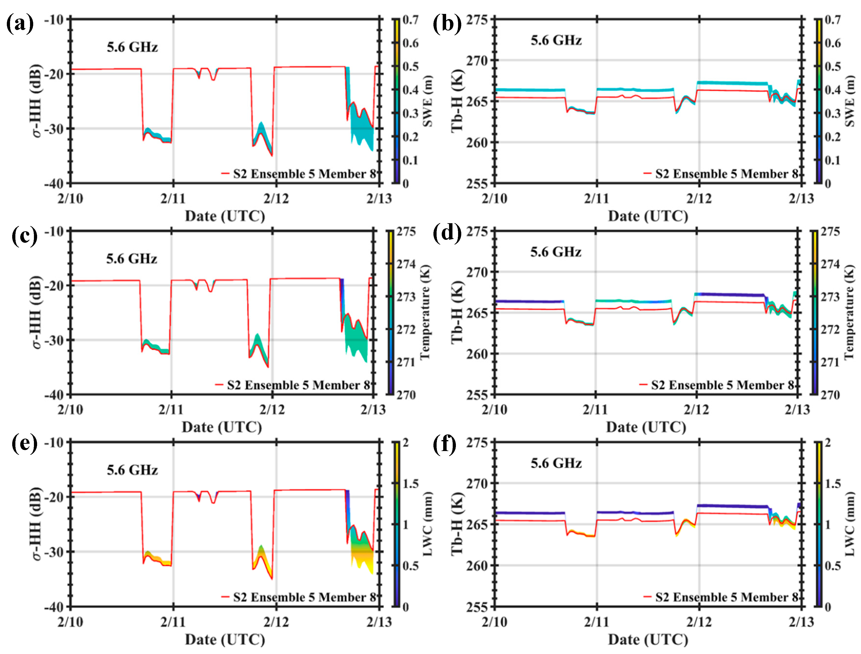
Figure 10 shows the temporal evolution of the backscattering coefficient σ HH- and σ VH-pol at 5.6 GHz and 1.3 GHz contoured by Ensemble 5 SWE during February 2017. The ensemble mean highlights the diurnal cycle of backscattering sensitivity that peaks in the afternoon when the spatial variability of HRRR radiative forcing and planetary boundary layer conditions is the highest. When daytime warming of the snowpack peaks causing surficial melt for some ensemble members. Note the much higher sensitivity overall at 5.6 GHz, including for high SWE ensemble members in the afternoon. The compound effect of the standard deviation of snow depth and snowpack condition explains the large range (up to 20 dB) among ensemble members (e.g., 2/12–2/17, 2/19–2/22, and 2/23). The decrease in uncertainty on 2/11, 2/17–2/18, and in the evening of 2/22 is due to the addition of fresh snow to the snowpack across the Mesa, as shown in Figure S12. Rain-on-snow for some of the ensemble members on 2/11 and 2/17–2/18 and hot air temperatures that cause surficial melting in other ensemble members enhance nighttime sensitivity at 5.6 GHz (e.g., Figure 11). Further, nighttime temperatures above the freezing point for some HRRR grids explain the differences in the snowpack’s nocturnal sensitivity between 5.6 GHz and 1.3 GHz in the evening of 2/10 and early morning of 2/11.
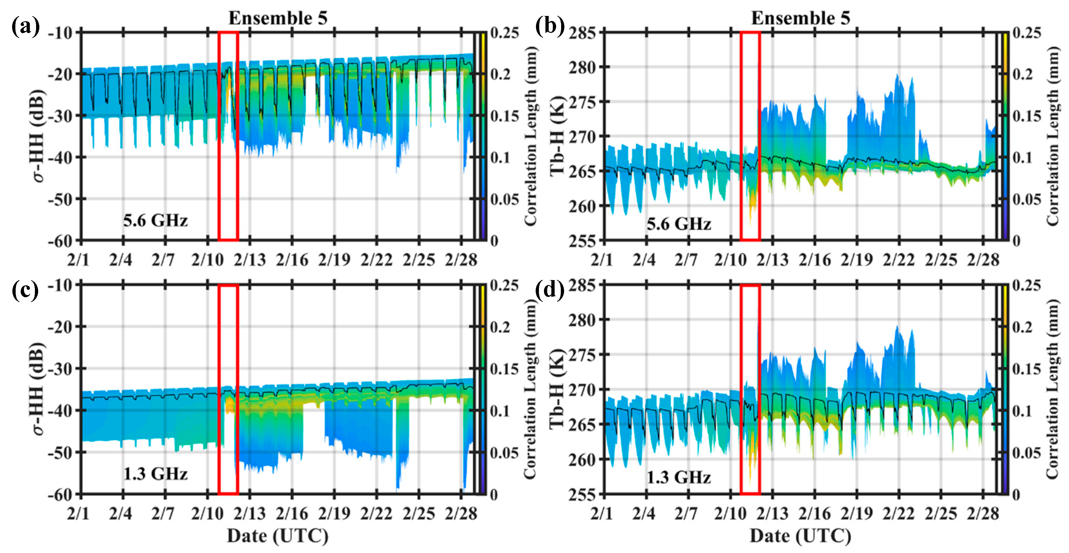
Figure 12 shows how melting during the second week of February reduces snowpack depth and SWE (Figure 8) and exposes deeper layers with longer snow correlation length (red box). The signature of long correlation lengths the top snowpack layer exposed by melt in the range of simulated backscatter in Figure 12 remains until the end of the month. However, it becomes smaller over time as new snowfall resets the top layer snow correlation length to much lower values. Nocturnal sensitivity (Figure 10 and Figure 12) collapses during the severe cooling event with intermittent snowfall at the end of the month (after 2/23). Daytime sensitivity peaks in the afternoon for some ensemble members, and at 5.6 GHz in particular as the weather begins to warm up on 2/26. The contrast between scattering behavior at 7 AM MST (similar for 7 PM LST) and 2 PM MST is illustrated in Figure S17 for January and February in 2017. At 7 AM MST, Ensemble 5 variance that captures the spatial variability attributed to meteorological forcing across the Grand Mesa at 3 × 3 km2 remains at, or below 3 dB for both 1.3 GHz and 5.6 GHz with very little difference between the two except on 9 January (bottom left), when a snowstorm produces a significant increase in snow depth. At 2 PM MST, the standard deviation does not significantly change at 1.3 GHz, but it increases up to 8 dB at 5.6 GHz tied to surface melt. Indeed, daytime snowmelt and subsequent nighttime refreeze previously identified by [9] in Grand Mesa using Sentinel 1, C-band (5.6 GHz) SAR measurements are the most important source of variability in the accumulation regime.
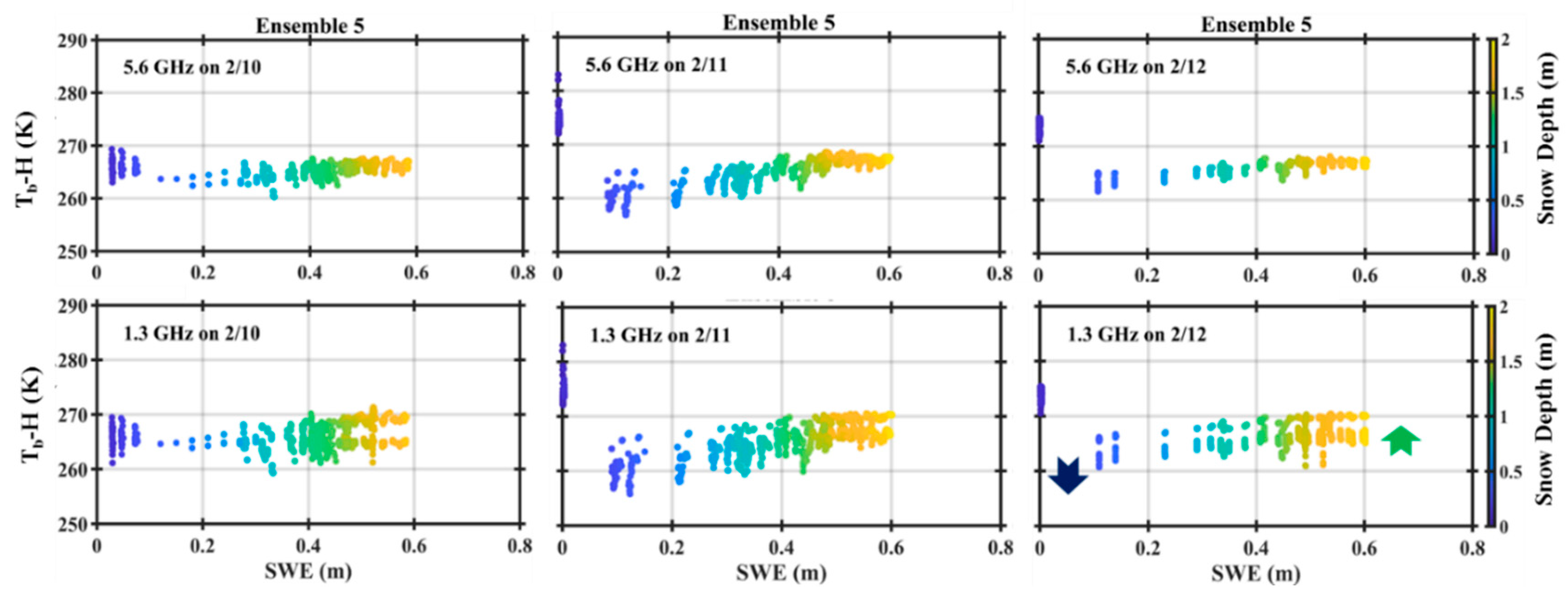
Interestingly, the amplitude of the impact of surface melting in daytime backscattering is the same across scales. For the case of EFF2, when the downscaled precipitation fields are used at 750 × 750 m2, there is little sensitivity to the spatial variability of precipitation at 1.3 GHz (not shown). In contrast, the spatial variability can be as high as 10 dB for 5.6 GHz even when snow depth and SWE differences are small at S2 due to daytime surficial snowpack melting in the second and third weeks of February (Figure S12). Due to cold temperatures, more considerable spatial variability of snow depth at the end of February does not propagate into the backscattering behavior of the snowpack. Figure 13 contrasts the interplay between snow and rainfall and air temperature at mid-day for the 3 days starting in 2/10 and ending on 2/12 when significant spatial variability in mid-day liquid water content (LWC) the top layer of the snowpack enhances the subgrid-scale spatial variability. Note how the mean backscatter at 5.6 GHz (Figure 13, left) and the ensemble range increase from 2/11 to 2/12 during daytime as expected due to the LWC decrease in the top layer of the snowpack in some of the ensemble members on 2/12. The broad EFF2 ensemble range on 2/12 also reflects the spatial variability of other snowpack physical properties, including snow depth, surface temperature, and microphysics. By contrast, the sensitivity of brightness temperatures at the subgrid-scale is minimal (Figure 13, right). Figure 14 shows high sensitivity (~10 K) of brightness temperatures (e.g., 1.3 and 5.6 GHz) for the same three-day period across Grand Mesa. Ambiguity in the relationship between SWE and Tb, or snow depth and Tb, is larger at 1.3 GHz and varies with time-of-day and snowpack condition (e.g., 2/11 vs. 2/12). Therefore, it is desirable for snow remote sensing to make either active or passive measurements early in the morning or late in the afternoon.
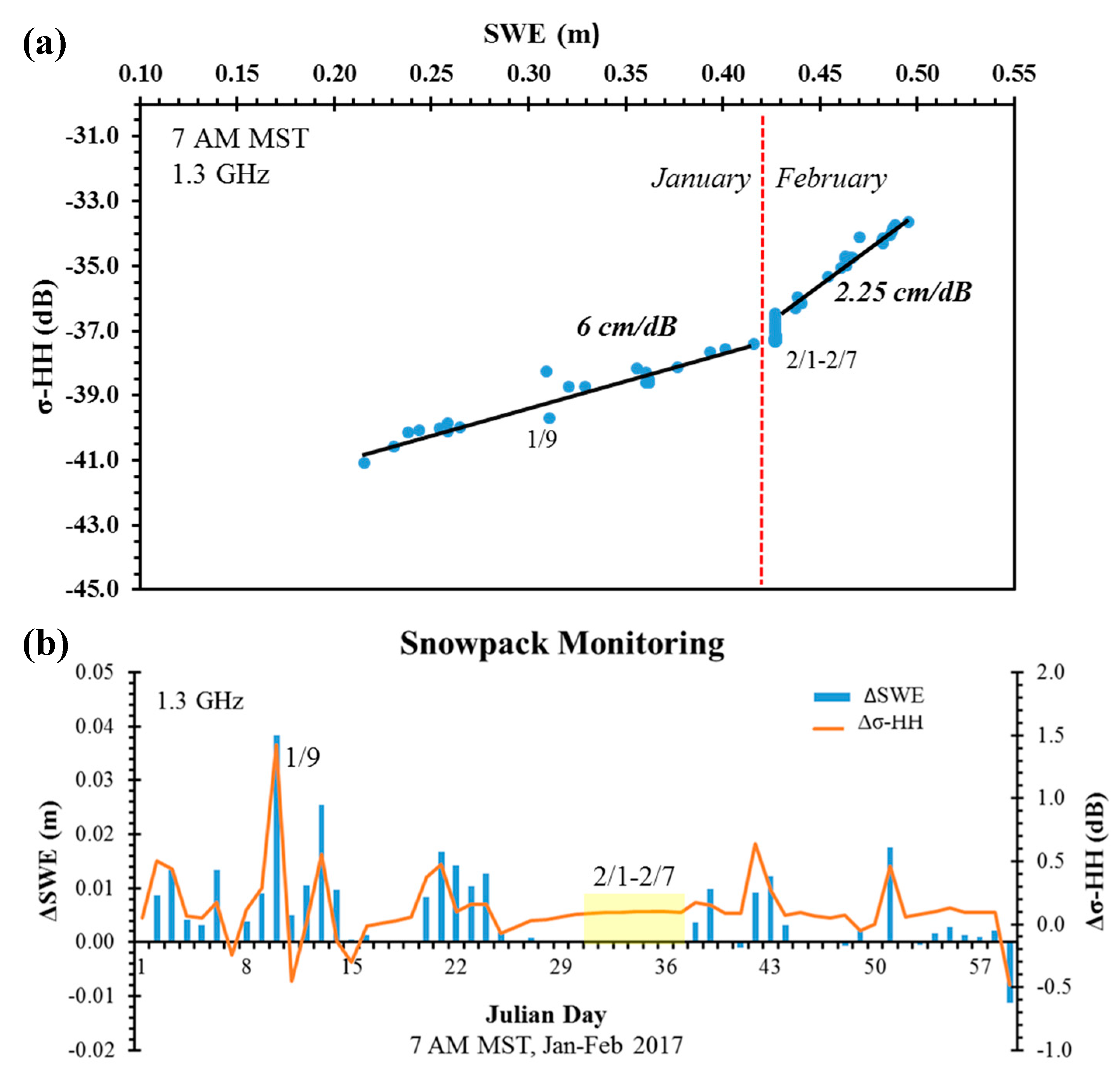
Figure 15 shows the simulated temporal evolution of Ensemble 5 mean σ-HH at 1.3 GHz at 7 AM MST from 1/1 through 2/28 in 2017 in terms of total snow accumulation and day-to-day changes. The corresponding results at 5.6 GHz are shown in Figure S19. The snowpack deepens in January due to cold weather and several snowstorms, corresponding to an increase in SWE as a function of σ-HH (ΔSWE/Δσ) of 5–6 cm/dB at the monthly time-scale. Figure S20 shows the temporal evolution of the standard deviation of Ensemble 5 members that increases in the aftermath of snowstorms and melt events, and decreases under cold conditions. The erratic weather in February results in much lower snow accumulation. Rapidly changing backscatter in the first week of the month is mainly attributed to microphysical changes in the top layer of the snowpack, followed by steady accumulation at a rate of ~2 cm/dB later in the month. This behavior demonstrates the time-integrated sensitivity of backscatter to regional weather during the seasonal snowpack accumulation phase. It implies that the specific history of weather and snowpack interactions determines the backscattering behavior. Therefore, it hints at the necessity of physically-based retrieval via, for example, data-assimilation for applications over large areas. Yurchak [52] relates (ΔSWE/Δσ) to the variance of the Fresnel coefficient in a layered snow medium, which in turn is proportional to the density variance. This approach explains the spatial variability of accumulation rates (2–10 cm/dB) from scatterometer data matching different snow types in Antarctica [26]. Using a 1-layer snow model and one-parameter at a time sensitivity analysis, Oveigharan et al. [53] showed that the backscattered power in dual-polarization dual-frequency retrievals at C- and Ku-bands is more sensitive to snow density and grain radius than to snow depth. This raises the possibility of retrieving information on snowpack stratigraphy. Furthermore, the time-matched history of consecutive changes in SWE (ΔSWE) and changes in backscatter (Δσ-HH) in Figure 15 and Figure S19 suggests that it is possible to use changes in backscatter to detect individual snowstorm activity and associated snowfall above a minimum threshold of Δσ (~0.3 dB/day).
The full evolution of the Ensemble 5 mean of simulated backscatter and brightness temperatures of the seasonal snowpack across Grand Mesa is shown respectively in Figure 16a,b from 9/1/2016 through 6/30/2017. Results for different polarizations at 7 AM MST and even at mid-day (2 PM MST), albeit complicated by mid-day melting, exhibit similar behavior (Figures S21 and S22).
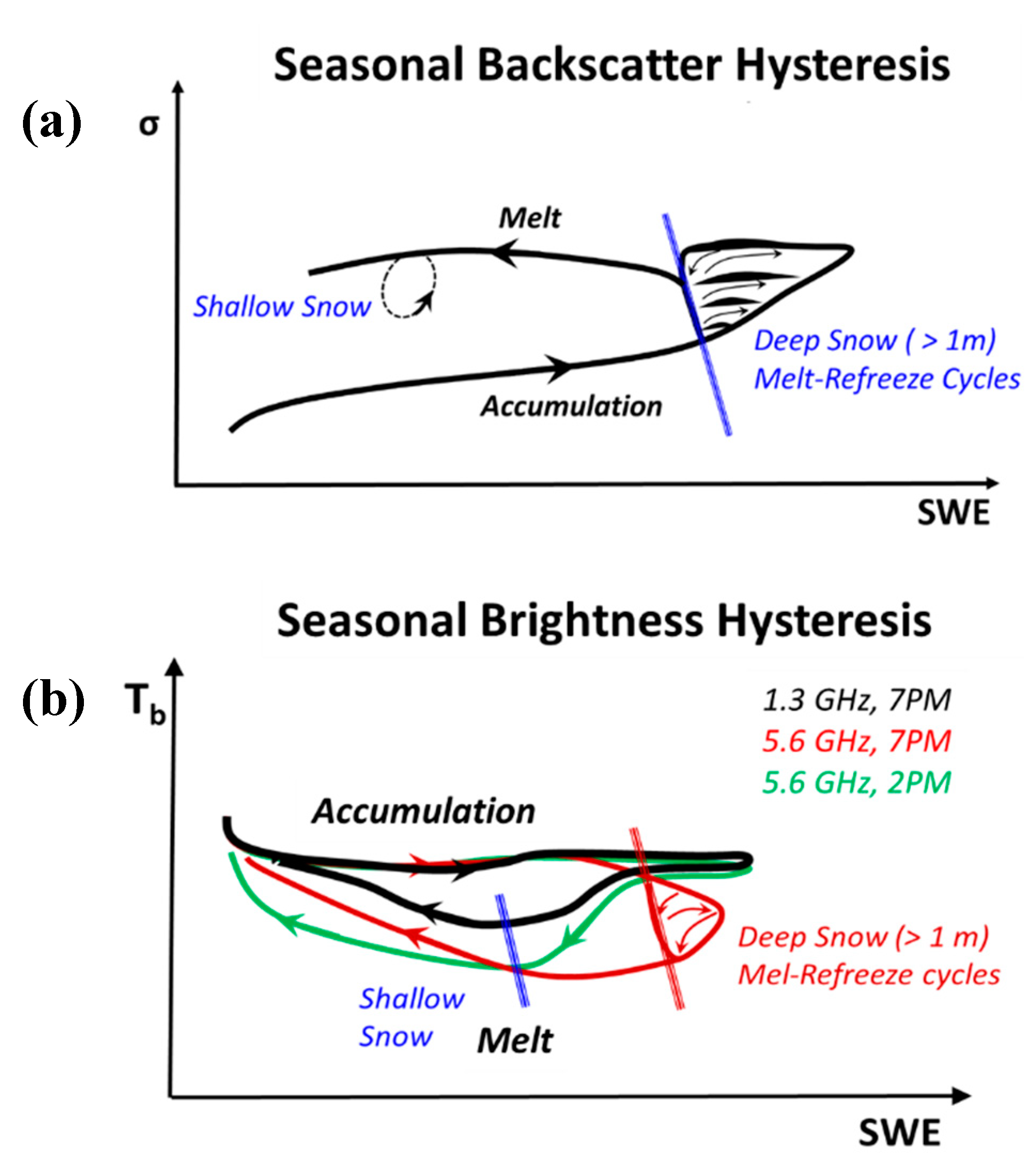
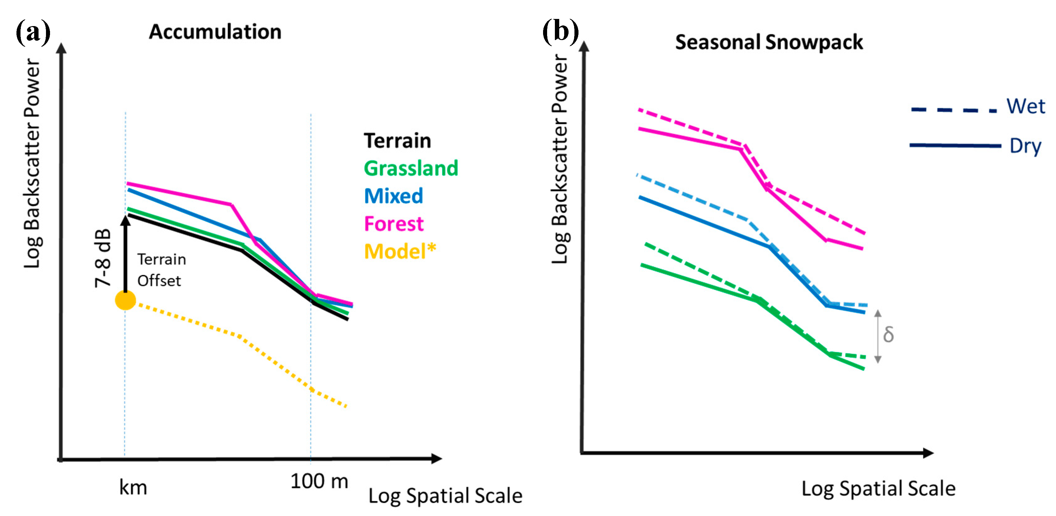
The conceptual diagram in Figure 17a synthesizes the temporal evolution of backscatter hysteresis between the accumulation and the melt phases. Evidence of nonlinear behavior is apparent in the winter-spring transition season with melt-refreeze cycles (April), and in the melting regime for deep snow as the snowpack ripens (May) and for ripe shallow snowpack conditions late in the season (June). Hysteretic backscatter offsets decrease with frequency increases and nearly collapse at Ku-band in the late spring’s melting regime. In this case, sensitivity to small changes in wet, shallow snowpacks introduces considerable uncertainty (i.e., noise). Although the range of conditions simulated here is limited by the simplicity of model assumptions and the strict focus on uncertainty tied to meteorological forcing and not to model structure or model parameters, the results suggest that there is potential to take advantage of hysteresis at lower frequencies (e.g., L- and C-band in the melting regime), and power at higher frequencies (e.g., Ku-band in the accumulation regime) to improve the signal-to-noise ratio in SWE remote sensing.
The temporal evolution of microwave emissions maps a closed trajectory (e.g., limit-cycle, Figure 16b) in the (Tb, SWE) phase-space that shows very little sensitivity during the accumulation phase when SWE >10 cm followed by large nonlinear sensitivity in the return phase with clear separation of the behavior of deep snow in the early winter-spring transition stage and shallow snow in late spring. This behavior is synthesized in Figure 17b. The transient cooling in early spring followed by warming in late spring is well documented in [21] for brightness temperatures at higher frequencies (up to 37 GHz). The differences in the hysteretic offsets at different frequencies establish a physical basis for the first heuristic remote sensing algorithms [15,16]. Because of nonlinear dynamic sensitivity and dramatic changes between early and late melt regimes, and because of sensitivity to seasonal weather at local and regional scales (e.g., Figure 15 and Figure S19), finding unique relationships for retrieval is challenging (i.e., calibration of model parameters may not be robust). Whereas soil emissions below the snow-soil interface are not accounted for here, previous point-scale studies of microwave emissions including the contribution of the soil substrate [53,54] indicate that between December 1 at the time the soil freezes and March 1 in this study, one would expect to see an increase in brightness temperatures on the order of 10K, followed by a decrease of the same order of magnitude in the spring when the soil substrate is fully thawed, which potentially amplifies the limit-cycles shown in Figure 16c and thus reduces ambiguity (Figure S23). Nevertheless, coupling snow hydrology and microwave models provides a framework for physically-based interpretation and disambiguation of microwave measurements of snowpack properties toward a monitoring system that can be achieved by data-assimilation.

5. Discussion

The signatures of the sub-seasonal variability of snow physics were investigated through forward modeling akin to an exploratory observing system simulation experiment (OSSE) in Grand Mesa. The co-evolution of radar backscattering coefficients and brightness temperatures at L- (1.3 GHz), C- (5.6 GHz), Ku- (13.5 GHz), and Ka- (35.7 GHz) bands were examined during snow accumulation and melting phases toward assessing their interpretability and sensitivity. At daily time-scales, during the accumulation season, the sensitivity to atmospheric forcing (i.e., spatial variability of weather within the Grand Mesa) remains below 3 dB for cold weather conditions (i.e., dry snow). It increases to 8–10 dB at midday when temperatures rise above freezing in the presence of surficial melt. Sub-grid scale variability of precipitation at 750 m in this study had a modest impact on snow depth, SWE, and backscatter in the accumulation regime for dry snow. However, microwave sensitivity increases by as much as 300% as small vertical snowpack structure differences are amplified when the liquid water content is present. Therefore, surficial melting is the process governing backscatter sensitivity to sub-grid scale variability. At mid-day, this sensitivity amounts to 3–10 dB of uncertainty measured by the standard deviation of the ensemble backscatter in Grand mesa, but it can be constrained below 3 dB if measurements are made early in the morning or late in the afternoon. Intermittent melt coupled with snow accumulation variability explains the wide range of the ensemble (~20 dB).
At monthly time-scales during the accumulation season, robust linear heuristic functional relationships between the ensemble mean backscatter and SWE can be found across the Grand Mesa (e.g., ~5–6 cm/dB in January; ~2–2.5 cm/dB in February at L- and C-bands). The nonstationary of these functional relationships reflects the cumulative impact of atmosphere-snowpack interactions over time, particularly melt-refreeze cycles that modify the microphysical and thermodynamic structure in the top 50 cm of the snowpack. This finding is consistent with conclusions by [9] using C-band SAR measurements from Sentinel-1.
The sensitivity behavior of active (up to 20 dB) and passive measurements (up to 15 K) to the spatial variability of weather conditions is very different depending on snowpack microphysics (Figure 12) and diurnal cycle of surficial melt (Figure 13). A multi-frequency multi-sensor snow retrieval algorithm can leverage these differences by adaptively selecting among available measurements that best discriminate the snowpack condition.
Analysis of full seasonal simulations reveals hysteresis in the mean backscatter behavior between accumulation and melt phases with hysteretic offsets that become noisier as frequency increases, especially for shallow and ripe snowpacks in late spring. The hysteretic behavior is captured by the temporal evolution of microwave emissions, with brightness temperatures following very distinct trajectories in the melting regime for deep and shallow snowpacks. These physical ties between snow hydrology and microwave behavior provide a physics-based framework to increase the potential for remote sensing of SWE through physical disambiguation of remotely-sensed microwave behavior. For instance, a multi-frequency approach to SWE measurement, which is conditional on snow state, could consist of using active Ku-band during the accumulation regime, and then by taking advantage of active and passive C- and, or L-band hysteresis in the melting regime (e.g., Figure 16a for σ-HH and σ-VH; Figure 16b for Tb-H and Tb-V). It also provides a framework for active-passive sensing, for instance, by making use of passive sensing in the accumulation regime to detect freeze-melt cycles (e.g., different between day-to-day changes in L- band backscatter and L-band brightness temperatures, Figure 16a and Figure 17a) and, or using active C-band or L-band in the early spring, followed by passive measurements in the late spring for shallow snowpacks (e.g., Figure 16b and Figure 17b). Ultimately, the optimal monitoring strategy reconciles existing technologies and can be explored via data-assimilation simulation studies to determine which measurements better constrain the coupled snow hydrology-radiative transfer model at different stages of the seasonal snowpack evolution.
Sub-grid scale effects of topography, land-cover, and, in particular, forests are not explicitly addressed in this study. A key question is whether compound uncertainty remains below 3 dB at the Grand Mesa scale (~300 km2), ~3 × 3 km2 resolution. Alternatively, their backscatter contribution can be isolated and parameterized. In addition to the neglecting land-cover and landform heterogeneity, snow metamorphism is represented by kinetic growth processes alone, and thus changes in snow correlation length due to depth and surface hoar formation as well as crusts formed due to melting refreeze or wind coarsening are not represented. Improvements in the representation of these processes will enhance confidence in the sensitivity analysis. The time-invariant backscatter at the snow-ground interface was forced to zero in the simulations (Table 2) to focus on the microwave signature of physical processes within the multi-layer snowpack. Depending on snow wetness conditions, a positive offset in the time-series of backscatter is expected that reflects local conditions (soils, land-cover, topography) at the spatial scale of the simulation. Scaling analysis [9] of Sentinel-1 C-band SAR backscatter suggests that snow-ground interactions can be accounted for by applying an offset at the spatial scale of measurement and using fractal disaggregation techniques to infer the fields at higher spatial resolution [42]. In Grand Mesa, the background offset can be estimated directly from snow-free measurements (7–8 dB, Figure S13). Robust scaling behavior over forest and mixed grassland and forest indicates potential to estimate the snow-background offset for different land-cover types during the accumulation and ablation seasons as illustrated in Figure 18. Nevertheless, it is important to stress that snow-soil and snow-vegetation interactions are not included in this analysis. While there is a good understanding of the microwave behavior of the soil-snow-vegetation-atmosphere (SSVA) system at point-scale from multi-frequency measurements and idealized model simulations (e.g., [55,56,57,58]), the spatial scaling behavior of microwave emission and backscatter from heterogeneous SSVA systems across different geographic regions and for different snow regimes is not well understood.

6. Conclusions

Ensemble predictions of the seasonal snowpack over Grand Mesa, CO, were conducted for the hydrologic year 2016–2017 using a multilayer snow hydrology model coupled to a microwave emission model. Atmospheric forcing ensembles were designed based on atmospheric reanalysis at 3 km spatial resolution, and exploratory simulations were conducted using fractal-downscaled precipitation between 3 km and 750 m. SWE and snow depth predictions driven by HRRR atmospheric forcing (EFF1, Ensemble 5; Table 1) at 3 km resolution show good agreement with snowpit observations. Despite neglecting topographic and land-cover variations across the Grand Mesa, the local bias SWE predictions are generally less than 50 mm (< 10% actual SWE, Figure 5 top panel) except at S1 and VS, where steep slopes and strong winds are expected to play an essential role in snow redistribution. The effect of uncertainty in snowfall, air temperature, and wind redistribution is apparent in the assessment of global bias (Figure 5 bottom panel). Overall, the modified Willmott Agreement Index (Appendix C) [59] that measures the agreement between the spread of the observations and model predictions is generally above 0.8, indicating model skill in space and time. The model performance meets the desired requirements for global observations from space by the Decadal Survey of Earth Sciences and Applications from Space [46] that is 10% uncertainty in SWE 3–5 km resolution. Thus, it is suitable to examine the uncertainty propagation from meteorological forcing to snowpack states to radiometric and scattering behavior with an eye toward remote sensing of SWE. Ultimately, the goal is to separate uncertainty in snowpack measurements from space (backscattering coefficient and brightness temperatures) from retrieval ambiguity tied to spatial scale, snow hydrology regime, and snow-soil-vegetation-atmosphere system heterogeneity.
The focus of this study is on high-elevation snowpack dynamics associated with snow physics separate from the soil substrate and vegetation cover. In the melting regime, independently of spatial scale and sub-grid scale variability, snow wetness alone introduces considerable ambiguities that can be addressed by probing the other snowpack states resolved in the snow hydrology model. Therefore, a coupled snow hydrology-radiative transfer approach should be advantageous toward systematic global implementation of SWE retrieval. Although only a limited number of frequencies and polarizations are analyzed in this study, and more systematic evaluations are needed to inform snow remote sensing, a critical implication of these results is that calibrated empirical or semi-empirical retrieval algorithms are not transferable from one location to another, or from one season to another.
The modeling framework can be implemented using other snow hydrology and radiative transfer models to explore realistic remote-sensing architectures systematically and for more complex landscapes. Specifically, future work will couple the snow hydrology model with improved snow metamorphism to other radiative transfer models (e.g., [52,60]) toward better characterizing uncertainty and examining nonlinear microwave behavior of heterogeneous snowpacks, including snow-soil and snow-vegetation interactions. One practical insight from this study is the suitability of adaptive monitoring strategies such as time-varying combinations of active and passive microwave at multiple frequencies to take advantage of unambiguous relationships (low uncertainty) between snowpack properties and the microwave signal conditional on snow regime.

Supplementary Materials

The following are available online at https://www.mdpi.com/2072-4292/12/20/3422/s1, Figure S1a. Numbering order convention for HRRR grid cells in Figure 1 (right panel) corresponding to the ID numbers in Table S1. HRRR grid cells were selected based on their proximity to the ECMWF grid cells’ center in Figure 1 (left panel). The red box delineates the grid cells used to discuss the results of the forward MEMLS simulations in Section 4.2. Figure S1b. Illustration of overlap of several HRRR Grids with one ECMWF grid, including hypothetical distribution of SnowEx’17 snowpits within the ECMWF grid. The diamonds are placed at the center of each grid. For example, HRRR grid 8 is the nearest to the center of the ECMWF grid corresponding to S2. In the context of ensemble simulations, we will refer to HRRR grid 8 as Ensemble Member 8. Figure S2. Structure of 1-D MHSM workflow. The first snowpack layer forms when the following two conditions are met: (1) The air temperature is below the freezing point (273.15 K); and (2) precipitation is present. In the melting season, liquid precipitation is added to the snowpack’s melting outflow directly. Figure S3. The geometry of the layered snowpack with an electromagnetic wave incident from above at an incidence angle θ n [37]. Notation: layer thickness d j , layer temperature T j , transmissivity t j , volume reflectivity r j , emissivity e j , and interface reflectivity s j , refracted angle θ j 1 for layer number j ranging from 1 (bottom) to n (top), snow-ground reflectivity s 0 and ground temperature T 0 . [ e j + r j + t j = 1 as required by energy conservation]. Figure S4. Schematic view of incoming and outgoing radiation between adjacent snow layers in MEMLS [37]. Notation as in Figure S2. Figure S5. HRRR snowfall (top panel), rainfall (mid panel), and near-surface air temperature (bottom panel) input to the MSHM from 9/1/2016 through 6/30/2017. The time-series are plotted in UTC = LST + 7. The blue line represents the ensemble mean of the 43 HRRR grids. The max-min envelope is marked in green, and yellow delimits the 25% and 75% of the 43 member ensemble. Figure S6. Illustration of recursive fractal precipitation downscaling scheme from 3km (HRRR resolution) to 750 m (see Figure S1b for notation). At each stage, 50 fields are generated, but only the ensemble mean downscaled to the next stage. Finally, the second ensemble family EFF2 for each ECMWF grid consisting of 16 members is generated with each member corresponding to one of the 16 ensembles means at 750 m resolution as precipitation input. In contrast, all other forcing and parameters in Table 1 are the same as EFF1 Ensemble 5. Figure S7. Time series of ensemble SWE predictions from 9/1/2016 through 6/30/2017 (left panels) and snow depth (right panels) for Ensemble 0, 1, 2, and 5 (Table 1) from top to bottom respectively. The blue dotted line is the ensemble mean. The green envelope identifies the ensemble range, and the yellow envelope delimits the 25th and 75th percentiles. Figure S8. Evaluation of predicted snow density and temperature profiles at S2 by Member 8 (HRRR grid point closest to the center of the S2 ECMWF grid point, Figure S1a) for Ensembles 1, 2, and 5 in the top, middle, and bottom rows respectively. The circles represent the average of snowpit density (left column, color scale on the right) and temperature (right column, color scale on the right) measurements as a function of depth (on the left-hand side y-axis) and date (x-axis). The measured values are plotted at the depth of measurement in the SnowEx’17 records. The model values are plotted at the mid-point of each layer. Time-series of simulated snowpack stratigraphy (number of layers and layer thickness) are provided in Supplementary Information (Figure S9a). Figure S9. MHSM predicted time-varying snowpack stratigraphy in terms of the number of layers and depth of the top layer during February 2017, corresponding to results presented in Figure 10 and Figure 11 for EFF1 Ensemble 5 for the ensemble members nearest the center of the ECMWF reference grids in Figure 1 (left panel): (a) ensemble member 8 at S2; (b) ensemble member 13 at SD3; and (c) ensemble member 29 at S5. The time-series are plotted in UTC = LST + 7. Figure S10. MSHM predicted time-series of temperature in the upper two layers of the snowpack (top row) and snowpack surface sensible heat flux (bottom row) at S2 for EFF1 Ensemble 5 Member 8. Specified air temperature from the HRRR model at grid 8 (Figure S1a) is provided for reference. The time-series are plotted in UTC = LST + 7. Figure S11. HRRR incoming longwave radiation flux during February 2017 at Grid 8 (Figure S1a). Time-series are plotted in UTC = LST + 7. Figure S12. Time series of HRRR analysis of near-surface (2 m) air temperature (top panel), snowfall (mid panel), and rainfall (bottom panel). The solid blue line represents the ensemble mean of the 43 HRRR grids (Figure S1); the green envelope captures the max and min values, and the yellow envelope marks the 25th and 75th percentiles. Figure S13. Comparison of Ensemble 5 simulated σ-HV (left column) and σ-VV (right column) at 5.6 GHz against the Sentinel-1 observations across the Grand Mesa on 7 February 2017 (top row) and 24 February 2017 (bottom row). For each violin diagram, the white dot represents the median; the black dashed bar marks the mean; the vertical black bar demarks the 25th and 75th percentiles; the upper and lower bounds represent the maximum and minimum values respectively; and finally, the colored contour is the density distribution. The 30-m Sentinel-1 data were averaged to 3 km within each of 43 HRRR grids. The red arrow shows the difference (7–8 dB) between the mean values, which is attributed to snow-ground interactions forced to zero in the simulations. The larger variance and range of Sentinel-1 illustrate the impact of land heterogeneities not represented in the simulations. Figure S14. Comparison of violin diagrams of Ensemble 5 Tb H-pol (left column) and V-pol (right column) on February 16, 2017, and continuous Surface-Based Radiometry (SBR) measurements [51] (https://nsidc.org/data/SNEX17_SBR/versions/1) at 10.65 GHz, 19 GHz, 36.5 GHz, and 89 GHz close to Pit 8 within ECMWF reference grid Ex (pink markers). For each violin diagram, the white dot represents the median; the red bar marks the mean; the vertical black bar demarks the 25th and 75th percentiles; the upper and lower bounds represent the maximum and minimum values, respectively; and finally, the colored contour is the density distribution. Markers follow the convention in Table S5. Figure S15. Same as Figure S14 on February 17 at Pits 17 and 5 (red markers) within ECMWF reference grids S5 and S4, respectively. Markers follow the convention in Tables S4 and S8, respectively. Figure S16. Evaluation of Ensemble 5 predictions of snow correlation length against values derived from snowpit grain size measurements following [52] within S2 on February 8, 9, and 10. The continuous lines represent Ensemble 5 mean values at three distinct times close to the reported time of snowpit measurements. The green envelope represents the min-max range of ensemble predictions at each depth. Markers follow the convention in Table S2. Figure S17. EFF1 Ensemble 5 variance of backscattering coefficients at 2 PM (top row) and 7 AM (bottom row) in January (left column) and February (right column) 2017 for snowpacks with depth > 10 cm. Figure S18. EFF2 at S2 snow depth (top left) during February 2017. The lines represent Ensemble 5 Member 8 behavior (top left). The EFF2 ensemble members between the 25th and 75th percentiles of the ensemble generated using downscaled precipitation at S2 fall in the yellow shaded region, and the green shade marks the minimum and maximum values. The remainder graphs present the corresponding time-series of backscattering coefficient σ-HH at 5.6 GHz contoured by SWE (top right), temperature (bottom left), and liquid water content LWC (bottom right) in the top layer of the snowpack. The light blue background shade marks the period of cold temperatures at the end of the month; the light orange background hade marks the warm period in the middle of the month. Figure S19. Snowpack monitoring in Grand Mesa at 5.6 GHz HH-pol during the accumulation season, January-February 2017. Top – Heuristic linear relationship between snowpack accumulation and backscatter (R2 > 0.95) that reflects the integration of variable weather conditions in January and February in the simulated snowpack. Bottom – SWE and backscatter increments, respectively ΔSWE and Δσ-HH, are calculated as the difference between today’s and yesterday’s values at 7 PM MST. MST- Mountain Standard Time = UTC - 7. Figure S20. Snowpack monitoring in Grand Mesa at 1.3 GHz HH-pol during the accumulation season, January-February 2017 corresponding to Figure 15 in the manuscript. Blue dots - Ensemble 5 mean values at the Grand Mesa scale. Orange squares- Standard deviation of the Ensemble 5 members. Figure S21. Seasonal evolution of Ensemble 5 mean backscatter σ-HH (left) and σ-HV (right) at 7 AM MST (bottom row) and 2 PM MST (top row) across the Grand Mesa throughout the snow season from 9/1/2016 through 6/30/2017. Figure S22. Seasonal evolution of Ensemble 5 mean brightness temperature Tb-H at 2 PM MST across the Grand Mesa throughout the snow season from 9/1/2016 through 6/30/2017. Figure S23. Idealized depiction of soil substrate impact on the seasonal evolution of brightness temperature emphasizing freeze-thaw processes and the effect of soil moisture after thaw. Table S1. Geographical correspondence between ECMWF and HRRR grids in Figure 1. Table S2. ECMWF reference grid S2: HRRR grid points (center of HRRR grid cell) and snowpit locations. Bold red letters identify the HRRR grid ID (Figure S1) nearest to the ECMWF grid center point. Table S3. Same as Table S2, but for ECMWF reference grid SD3. Table S4. Same as Table S2, but for ECMWF reference grid S5. Table S5. Same as Table S2, but for ECMWF reference grid Ex. Table S6. Same as Table S2, but for ECMWF reference grid S1. Table S7. Same as Table S2, but for ECMWF reference grid S3. Table S8. Same as Table S2, but for ECMWF reference grid S4. Table S9. Same as Table S2, but for ECMWF reference grid SD2. Table S10. Same as Table S2, but for ECMWF reference grid VS.

Author Contributions

A.P.B. designed the research and analysis; Y.C. processed data, carried out model simulations, and conducted quantitative analysis under the guidance of A.P.B.; A.P.B. and Y.C. wrote the manuscript cooperatively. All authors have read and agreed to the published version of the manuscript.

Funding

This research was funded by NASA’s Terrestrial Hydrology Program under NASA grant NNX17AL44G with the corresponding author.

Acknowledgments

The authors appreciate the National Snow & Ice Data Center for providing the NASA 2017 SnowEx data and all the colleagues who worked on the field campaign to collect the valuable data sets. The authors also appreciate reviewers’ valuable suggestions for improving the manuscript.

Conflicts of Interest

The authors declare no conflict of interest.

Appendix A. The Multilayer Snow Hydrology Model (MSHM)

The MSHM simulates snow hydrological processes in the snowpack column and quantifies energy and water fluxes at the land-atmosphere interface driven by meteorological forcing. The flowchart of model components and how they are connected is depicted in Supplementary Figure S2. The model formulation used in this manuscript is described here; additional implementation details and alternative parameterizations can be found in [20,21]. Units for each variable are in ().

Appendix A.1. Compaction

When SWE changes due to snowmelt, sublimation, rain-on-snow events, and snowfall, the snow depth h s n o w (m) is decreased by the compaction ratio C R (1/s) that is parameterized with metamorphism and overburden effects as follows:
C R = | 1 h s n o w d Δ h s n o w d t | metamorphism + | 1 h s n o w d Δ h s n o w d t | overburden
| 1 h s n o w d Δ h s n o w d t | metamorphism = 2.778 × 10 6 × C × e 0.04 × ( T s n o w   T i )
| 1 h s n o w d Δ h s n o w d t | overburden = P s n o w η × e 0.08 × ( T s n o w   T i ) × e 0.021 × ρ s n o w
where
C = { 1 ρ s n o w 150   k g / m 3 2 × e 0.046 × ( ρ s n o w 150 ) ρ s n o w > 150   k g / m 3
η is the viscosity coefficient at T i   ( = 273.15   K ) , P s n o w is the pressure due to the snowpack weight (N/m2), and ρ s n o w and T s n o w are the snow density (kg/m3) and temperature (K), respectively.

Appendix A.2. Snowpack Temperature

The heat energy transfer equation is
c s n o w × ρ w × h s w e × T s n o w t = K s n o w × T s n o w z + ϕ
in which ρ w   ( = 1000   k g / m 3 ) is the water density, c s n o w is the specific heat capacity of the snowpack (J/kg/K), and heat conductivity of the snowpack K s n o w (W/m/K) is calculated by
K s n o w = K a + ( 7.75 × 10 5 × ρ g s + 1.105 × 10 5 × ρ g s 2 ) × ( K i K a )
where K i and K a are, respectively, the heat conductivity of ice and air (W/m/K), ρ g s is the snow density-weighted by SWE h s w e (m) and liquid water content L W C (m):
ρ g s = ρ s n o w × h s w e L W C h s w e
The external forcing term ϕ (W/m2) is null except at the bottom and at the top layer of the snowpack. For the bottom layer:
ϕ = K s s × T s o i l T s n o w h s o i l + h s n o w
K s s , T s o i l and h s o i l are the heat conductivity at the snow-soil interface (W/m/K), superficial soil temperature (K), and soil depth (m), respectively. For the top layer:
ϕ = N S R + N L R + S + L
The net shortwave radiation flux N S R (W/m2) and the net longwave radiation flux N L R (W/m2) equal to
N S R = S W × ( 1 A l b )
N L R = L W ε × σ × T s n o w 4
S W and L W are the downward shortwaves and longwave radiation flux (W/m2), A l b and ε are the surface albedo and emissivity, respectively, and σ is the Stefan-Boltzmann constant.
Then, the sensible heat flux S (W/m2) is estimated by the air specific heat capacity c a (J/kg/K), air density ρ a (kg/m3), air temperature T a (K) and windspeed U (m/s) like:
S = c a × ρ a × C D T × U × ( T a T s n o w )
while the latent heat flux L (W/m2) is the product of air density, latent heat of vaporization L v (J/kg) and sublimation rate S (m/s):
L = ρ a × L v × S
and S is adapted by the Penman-Monteith equation:
S = Δ × ( N S R + N L R ) + γ × L v × ρ a × C D T × U × ( q a q s n o w * ) ρ w × L v × [ Δ + γ × ( 1 + C D T ) ]
where q a is the specific humidity (kg/kg) of air and Δ (Pa/K) that is the slope of saturation-vapor versus temperature curve at the air temperature can be approximated as:
Δ = e s n o w * e a * T s n o w T a
of which the saturated vapor pressure of snow e s n o w * and air e a * are expressed similarly:
e s n o w * = 611.2 × e x p [ 17.67 × ( T s n o w T i ) T s n o w T i + 243.5 ]
e a * = 611.2 × e x p [ 17.67 × ( T a T i ) T a T i + 243.5 ]
The psychrometric constant γ (Pa/K) and the snowpack’s saturated specific humidity q s n o w *   (kg/kg) are calculated by
γ = c a × P a 0.622 × L v
q s n o w * = 0.622 × e s n o w * P a
where P a (Pa) is the air pressure.

Appendix A.3. Conductance Factor and Aerodynamic Drag Coefficient

The parameterization of the conductance factor C D T in Equations (A11) and (A13) is like:
C D T = 1 R s n o w + 1 A
of which the snow surface resistance R s n o w is defined as a piecewise function of S W :
R s n o w = { 100 S W 50   W / m 2 1000 S W < 50   W / m 2
and aerodynamic drag coefficient A is from [61]:
A = 0.16 ( ln z z r ) 2 × ( 1 b × R i 1 + c × R i )
here z (m) is the height at which the windspeed U is and z r (m) is the roughness height of snow; b and c are coefficients depending on stability conditions: b = 1 and c = 4.7 when the boundary layer is stable ( R i > 0.25 ); whereas b = 9.4 and
c = 5.3 × 0.16 ( ln z z r ) 2 × b × z z r
for the unstable boundary layer ( R i 0.25 ).
Besides, the Richardson number R i is given by
R i = 9.81 × z × ( θ a θ s n o w ) U 2 × θ a + θ s n o w 2
of which θ a and θ s n o w are the potential temperature (K) of air and top layer snow, which are calculated as follows ( 1.02 × 10 5 Pa is the standard atmospheric pressure):
θ a = T a ( 1.02 × 10 5 P a ) 0.286
θ s n o w = T s n o w ( 1.02 × 10 5 P a ) 0.286

Appendix A.4. Melt

Snowpack melting is triggered when the energy need to melt snowpack ( Q m e l t ) exceeds 0, and Q m e l t (J/m2) are the sum of the net heat flux N H F L and the snowpack “cold content.” Q c c :
Q m e l t = N H F L + Q c c
where N H F L (J/m2) is the product of the MSHM’s time step size Δ t (s) and forcing terms on the right-hand side of Equation (A4):
N H F L = Δ t × ( K s n o w × T s n o w z + ϕ )
while Q c c (J/m2) is written as:
Q c c = c s n o w × ρ w × h s w e × ( T s n o w T i )
Furthermore, the melting occurs in two phases: ripening and deep melting, for which the snowpack both becomes isothermal (i.e., T s n o w = T i ) and the criteria are based on the difference between Q m e l t and Q r i p e n (J/m2) which is the energy need to ripen the snowpack:
Q r i p e n = L m × ρ w × L W C m a x
here L m (J/kg) is the latent heat for melting and L W C m a x (m) that depends on ρ s n o w and h s n o w is the maximum liquid water content retained in the pore spaces against gravity by surface tension forces of snow grains:
L W C m a x = { 0.01 × h s n o w ρ s n o w < 400   k g / m 3 ( 0.25 × ρ s n o w ρ w 0.099 ) × h s n o w ρ s n o w 400   k g / m 3
Ripening happens when Q m e l t < Q r i p e n , under which there is no water melting out and the internal L W C is proportional to L W C m a x :
L W C = L W C m a x × Q r i p e n Q m e l t Q r i p e n
On the contrary, deep melting takes place and initiates the meltwater h m e l t (m):
h m e l t = Q m e l t Q r i p e n L m × ρ w
by which the diminution of SWE Δ h s w e (m) and L W C are determined:
Δ h s w e = { h s w e h m e l t h s w e h m e l t L W C m a x L W C m a x h m e l t < h s w e 0 h m e l t < L W C m a x
L W C = { 0 h m e l t h s w e L W C m a x L W C m a x h m e l t < h s w e h m e l t h m e l t < L W C m a x
Note the liquid water capacity is reached on the second condition, hence Δ h s w e is actually the infiltration or runoff released from the snowpack, and the snowpack is completely melted in the first case ( h m e l t h s w e ), so there is no L W C left, whereas all meltwater is held within the snowpack in the last one.

Appendix A.5. Rain-on-Snow

A rain-on-snow event only occurs when the rainfall rate P r is not nil, and air temperature T a is above freezing point ( T i ), in which case only the top-layer snow will be influenced, and its status is dependent on the thermodynamic energy of snowpack ( E s n o w ) and rain ( E r a i n ), both of which consist of different components:
E s n o w = Q c c + Q r i p e n H r i p e n + L m × ρ w × h s w e H m e l t
where H r i p e n (J/m2) and H m e l t (J/m2) are the heat released from the rain to ripen and melt the snow layer, respectively.
E r a i n = c w × M r × ( T a T i ) Q w c + L m × M r H f r o
here Q w c (J/m2) is the “warm content” of the rainfall and H f r o (J/m2) is the released heat after the raindrop becomes frozen. c w is the specific heat capacity of water (J/kg/K) and M r is the rainfall mass (kg/m2) during a model’s time step (i.e., the product of P r and Δ t ).
The warm rainfall would melt the top-layer snow completely in two cases: E r a i n E s n o w or H r i p e n E r a i n < E s n o w Under both circumstances, falling rain joins the snowpack’s melting outflow directly. On the other hand, when E r a i n Q c c . All rain freezes and adds to the snowpack mass with releasing energy to raise the snowpack temperature by Δ T s n o w (K):
Δ T s n o w = ( T i T s n o w ) × ( E r a i n Q c c 1 + M r ρ w × ρ i h s w e × ρ w 2 )
among which 1 and 2 marking the fractional increase toward T i are the adjusting term of energy and mass, respectively, while the boxed item is the increment of snow mass (SWE). ρ i is the ice density (kg/m3).
If E r a i n < H r i p e n or Q w c Q c c The rain will be absorbed by the isothermal mushy snowpack and promote h s w e by the same magnitude in Equation (A38), as well as L W C by Δ L W C (m):
Δ L W C = min ( M r ρ w , L W C m a x L W C )

Appendix A.6. Dividing and Combining Snow Layers

The MSHM will activate the dividing mechanism, which only separates the top-layer snow into n + 1 new layers and specifies their properties, without acting on the lower layers beneath the top one, if the round ratio ( n ) of top-layer SWE to a specific threshold ( T h r e s ) is greater than 1:
n = f l o o r ( h s w e T h r e s )
in which the f l o o r operation rounds the fraction to the nearest integer less than or equal to it.
As presented in Figure S2, the snow properties from the layer m to m + n remain the same with the original top layer after the dividing behavior:
ρ s n o w m + n = = ρ s n o w m + 1 = ρ s n o w m
T s n o w m + n = = T s n o w m + 1 = T s n o w m
L c m + n = = L c m + 1 = L c m
except for snow depth and SWE:
h s n o w m + n 1 = = h s n o w m + 1 = H s n o w m = T h r e s × ρ w ρ s n o w m
h s w e m + n 1 = = h s w e m + 1 = H s w e m = T h r e s
h s w e m + n = h s w e m T h r e s × n
h s n o w m + n = h s w e m + n × ρ w ρ s n o w m
On the other hand, when the snow depth h s n o w j at layer j is less than or equal to a critical value, the MSHM will combine all mass-related terms, such as h s n o w j and h s w e j , with the lower layer j 1 :
h s n o w j = h s n o w j + h s n o w j 1
h s w e   j = h s w e j + h s w e j 1
whereas ρ s n o w j , T s n o w j and L c j are averaged and weighted by SWE through two consecutive snow layers:
ρ s n o w j = h s w e j × ρ s n o w j + h s w e j 1 × ρ s n o w j 1 h s w e j + h s w e j 1
T s n o w j = h s w e j × T s n o w j + h s w e j 1 × T s n o w j 1 h s w e j + h s w e j 1
L c j = h s w e j × L c j + h s w e j 1 × L c j 1 h s w e j + h s w e j 1

Appendix A.7. Snow Correlation Length

The temporal evolution of snow correlation length L c j in layer j is calculated based on the kinetic grain growth rate adapted from [62] as follows:
d L c j d t = S P × ( A 1 + A 2 L c j ) × e A 3 × ( 1 T i 1 T s n o w j ) × α × 1000
where A 1 = 5.9 × 10 12 m/s, A 2 = 9.4 × 10 17 m2/s, A 3 = 2.9 × 10 3   K , S P   ( = 1 ) is the sphericity, and α   ( = 6 ) is based on the optimal relationship between correlation length and grain diameter reported by [63].

Appendix B. The Microwave Emission Model of Layered Snowpacks (MEMLS)

MEMLS was developed based on the six-flux theory to simulate multiple volume scattering and absorption, which contains radiation trapping resulted from internal reflections and coherent ones between layer interfaces. It was first implemented to simulated brightness temperatures [36] and recently expanded to simulate backscattering [35]. The latter made their code publicly available, and we use it in this work.
In MEMLS, the snowpack is described as a column consisting of n horizontal layers (j = 1, 2 … n) with flat boundaries at the surface and interfaces between layers. Each layer is characterized by layer thickness, transmissivity, density, reflectivity, emissivity, and temperature that determine the observed snowpack brightness temperature T b given by the sky brightness temperature T s k y (Figure S3).
As illustrated by Figure S4, the outgoing radiation ( A j and D j ) from layer j and the incoming radiation ( B j and C j ) can be expressed as follows:
A j = r j B j + t j C j + e j T j
D j = t j B j + r j C j + e j T j
B j = s j 1 A j + ( 1 s j 1 ) D j 1
C j = ( 1 s j ) A j + 1 + s j D j
where D 0 (when j = 1 ) on the right-hand side of Equation (A56) is defined as the ground temperature T 0 ; while A n + 1 (when j = n ) on the right-hand side of Equation (A57) is given by the downwelling sky radiation T s k y . Similarly, we can derive the main model output-the whole snowpack brightness temperature T b from
T b = B n + 1 = s n T s k y + ( 1 s n ) D n
D n can be determined by substituting Equations (A56) and (A57) into Equations (A54) and (A55):
A j = r j [ s j 1 A j + ( 1 s j 1 ) D j 1 ] + t j [ ( 1 s j ) A j + 1 + s j D j ] + e j T j
D j = t j [ s j 1 A j + ( 1 s j 1 ) D j 1 ] + r j [ ( 1 s j ) A j + 1 + s j D j ] + e j T j
This coupled linear system of equations can be written in matrix form:
A = M 1 A + M 2 D + E
D = M 3 A + M 4 D + F
among which M 1 , M 2 , M 3 and M 4 are n × n matrices including reflectivity r , transmissivity t , and emissivity e ; E and F are n × 1 vectors containing boundary T s k y and surface temperature T 0 .
After linear algebra, the final expression for D is
D = ( I M 5 ) 1 [ M 3 ( I M 1 ) 1 E + F ]
where I is the identity matrix and M 5 is
M 5 = M 3 [ ( I M 1 ) 1 M 2 ] + M 4

Appendix C. Modified Wilmott Agreement Index [59]

W A I d , p l o c a l = 1 ( y d , p x ¯ d , p ) 2 × 1 N s ( d , p ) s = 1 N s ( d , p ) ( x d , p s x ¯ d , p ) 2 + 1 N r r = 1 N r ( y ¯ d x ¯ d , p ) 2  
W A I d , p g l o b a l = 1 ( y ¯ d x ¯ d , p ) 2 × 1 N s ( d , p ) s = 1 N s ( d , p ) ( x d , p s x ¯ d , p ) 2 + 1 N r r = 1 N r ( y ¯ d x ¯ d , p ) 2  
y d , p is the model SWE (or snow depth) simulated over the HRRR grid that is nearest to the ECMWF grid point p on day d at time t = Tref, where Tref = 10 AM LST = 17:00 UTC;
  • N r (=43) is the number of HRRR grids;
  • N s ( d , p ) is the number of snowpits within pixel p on day d, which is different for each pixel p;
  • x d , p s is the observed SWE (or snow depth) at site s within pixel p on day d;
  • x ¯ d , p is the mean of the observations from all sites within pixel p on day d;
  • y ¯ d is the ensemble mean on day d at time t = Tref.

References

  1. Hall, D.K. Assessment of Polar Climate Change Using Satellite Technology. Rev. Geophys. 1988, 26, 26–39. [Google Scholar] [CrossRef]
  2. Barnett, T.P.; Dumenil, L.; Schlese, U.; Roeckner, E.; Latif, M. The Effect of Eurasian Snow Cover on Regional and Global Climate Variations. J. Atmos. Sci. 1989, 46, 661–685. [Google Scholar] [CrossRef] [Green Version]
  3. Chapin, F.S.; Sturm, M.; Serreze, M.C.; McFadden, J.P.; Key, J.R.; Lloyd, A.H.; McGuire, A.D.; Rupp, T.S.; Lynch, A.H.; Schimel, J.P.; et al. Role of land-surface changes in Arctic summer warming. Science 2005, 310, 657–660. [Google Scholar] [CrossRef] [PubMed]
  4. Gustafsson, D.; Stahli, M.; Jansson, P.E. The surface energy balance of a snow cover: Comparing measurements to two different simulation models. Theor. Appl. Climatol. 2001, 70, 81–96. [Google Scholar] [CrossRef]
  5. Lemke, P.; Ren, J.; Alley, R.B.; Allison, I.; Carrasco, J.; Flato, G.; Fujii, Y.; Kaser, G.; Mote, P.; Thomas, R.H. Observations: Changes in Snow, Ice and Frozen Ground. 2007. Available online: http://ecite.utas.edu.au/100647 (accessed on 22 May 2015).
  6. Albert, M.R. Effects of snow and firn ventilation on sublimation rates. Ann. Glaciol. Ser. 2002, 35, 52–56. [Google Scholar] [CrossRef]
  7. Barnett, T.P.; Adam, J.C.; Lettenmaier, D.P. Potential impacts of a warming climate on water availability in snow-dominated regions. Nature 2005, 438, 303–309. [Google Scholar] [CrossRef]
  8. Painter, T.H.; Skiles, S.M.; Deems, J.S.; Brandt, W.T.; Dozier, J. Variation in Rising Limb of Colorado River Snowmelt Runoff Hydrograph Controlled by Dust Radiative Forcing in Snow. Geophys. Res. Lett. 2018, 45, 797–808. [Google Scholar] [CrossRef] [Green Version]
  9. Manickam, S.; Barros, A. Parsing Synthetic Aperture Radar Measurements of Snow in Complex Terrain: Scaling Behaviour and Sensitivity to Snow Wetness and Landcover. Remote Sens. 2020, 12, 483. [Google Scholar] [CrossRef] [Green Version]
  10. Schmugge, T.J.; Kustas, W.P.; Ritchie, J.C.; Jackson, T.J.; Rango, A. Remote sensing in hydrology. Adv. Water Resour. 2002, 25, 1367–1385. [Google Scholar] [CrossRef]
  11. Tedesco, M.; Kelly, R.E.J.; Foster, J.L.; Chang, A.T.C. AMSR-E/Aqua Daily L3 Global Snow Water Equivalent EASE-Grids V002; National Snow and Ice Data Center: Boulder, CO, USA, 2004. [Google Scholar]
  12. Lettenmaier, D.P.; Alsdorf, D.; Dozier, J.; Huffman, G.J.; Pan, M.; Wood, E.F. Inroads of remote sensing into hydrologic science during the WRR era. Water Resour. Res. 2015, 51, 7309–7342. [Google Scholar] [CrossRef]
  13. Hall, D. Passive Microwave Studies of Snowpack Properties; Goddard Space Flight Center: Greenbelt, MD, USA, 1978. [Google Scholar]
  14. Hall, D.; Foster, J.; Chang, A.; Rango, A. Passive microwave applications to snowpack monitoring using satellite data. 1979. Available online: https://ntrs.nasa.gov/citations/19790020478 (accessed on 3 September 2013).
  15. Rango, A.; Chang, A.; Foster, J. The utilization of spaceborne microwave radiometers for monitoring snowpack properties. Hydrol. Res. 1979, 10, 25–40. [Google Scholar] [CrossRef]
  16. Chang, A.; Foster, J.; Hall, D.K. Nimbus-7 SMMR derived global snow cover parameters. Ann. Glaciol. 1987, 9, 39–44. [Google Scholar] [CrossRef] [Green Version]
  17. Grody, N.C.; Basist, A.N. Global identification of snowcover using SSM/I measurements. IEEE Trans. Geosci. Remote Sens. 1996, 34, 237–249. [Google Scholar] [CrossRef]
  18. Tait, A.B. Estimation of snow water equivalent using passive microwave radiation data. Remote Sens. Environ. 1998, 64, 286–291. [Google Scholar] [CrossRef]
  19. Andreadis, K.M.; Liang, D.; Tsang, L.; Lettenmaier, D.P.; Josberger, E.G. Characterization of errors in a coupled snow hydrology-microwave emission model. J. Hydrometeorol. 2008, 9, 149–164. [Google Scholar] [CrossRef] [Green Version]
  20. Kang, D.H.; Barros, A.P. Observing System Simulation of Snow Microwave Emissions Over Data Sparse Regions-Part I: Single Layer Physics. IEEE Trans. Geosci. Remote Sens. 2012, 50, 1785–1805. [Google Scholar] [CrossRef]
  21. Kang, D.H.; Barros, A.P. Observing System Simulation of Snow Microwave Emissions Over Data Sparse Regions-Part II: Multilayer Physics. IEEE Trans. Geosci. Remote Sens. 2012, 50, 1806–1820. [Google Scholar] [CrossRef]
  22. Kang, D.H.; Barros, A.P.; Dery, S.J. Evaluating Passive Microwave Radiometry for the Dynamical Transition From Dry to Wet Snowpacks. IEEE Trans. Geosci. Remote Sens. 2014, 52, 3–15. [Google Scholar] [CrossRef]
  23. Tedesco, M.; Kim, E.J.; England, A.W.; De Roo, R.D.; Hardy, J.P. Brightness Temperatures of Snow Melting/Refreezing Cycles: Observations and Modeling Using a Multilayer Dense Medium Theory-Based Model. IEEE Trans. Geosci. Remote Sens. 2006, 44, 3563–3573. [Google Scholar] [CrossRef]
  24. Foster, J.L.; Sun, C.J.; Walker, J.P.; Kelly, R.; Chang, A.; Dong, J.R.; Powell, H. Quantifying the uncertainty in passive microwave snow water equivalent observations. Remote Sens. Environ. 2005, 94, 187–203. [Google Scholar] [CrossRef]
  25. Langlois, A.; Royer, A.; Derksen, C.; Montpetit, B.; Dupont, F.; Goita, K. Coupling the snow thermodynamic model SNOWPACK with the microwave emission model of layered snowpacks for subarctic and arctic snow water equivalent retrievals. Water Resour. Res. 2012, 48, W12524. [Google Scholar] [CrossRef] [Green Version]
  26. Rotschky, G.; Rack, W.; Dierking, W.; Oerter, H. Retrieving snowpack properties and accumulation estimates from a combination of SAR and scatterometer measurements. IEEE Trans. Geosci. Remote Sens. 2006, 44, 943–956. [Google Scholar] [CrossRef]
  27. Raleigh, M.S.; Lundquist, J.D.; Clark, M.P. Exploring the impact of forcing error characteristics on physically based snow simulations within a global sensitivity analysis framework. Hydrol. Earth Syst. Sci. 2015, 19, 3153–3179. [Google Scholar] [CrossRef] [Green Version]
  28. Larue, F.; Royer, A.; De Sève, D.; Roy, A.; Picard, G.; Vionnet, V.; Cosme, E. Simulation and assimilation of passive microwave data using a snowpack model coupled to a calibrated radiative transfer model over northeastern Canada. Water Resour. Res. 2018, 54, 4823–4848. [Google Scholar] [CrossRef]
  29. Xue, Y.; Forman, B.A.; Reichle, R.H. Estimating Snow Mass in North America Through Assimilation of Advanced Microwave Scanning Radiometer Brightness Temperature Observations Using the Catchment Land Surface Model and Support Vector Machines. Water Resour. Res. 2018, 54, 6488–6509. [Google Scholar] [CrossRef]
  30. Dechant, C.; Moradkhani, H. Radiance data assimilation for operational snow and streamflow forecasting. Adv. Water Resour. 2011, 34, 351–364. [Google Scholar] [CrossRef]
  31. De Lannoy, G.J.M.; Reichle, R.H.; Arsenault, K.R.; Houser, P.R.; Kumar, S.; Verhoest, N.E.C.; Pauwels, V.R.N. Multiscale assimilation of Advanced Microwave Scanning Radiometer-EOS snow water equivalent and Moderate Resolution Imaging Spectroradiometer snow cover fraction observations in northern Colorado. Water Resour. Res. 2012, 48, W01522. [Google Scholar] [CrossRef]
  32. Charrois, L.; Cosme, E.; Dumont, M.; Lafaysse, M.; Morin, S.; Libois, Q.; Picard, G. On the assimilation of optical reflectances and snow depth observations into a detailed snowpack model. Cryosphere 2016, 10, 1021–1038. [Google Scholar] [CrossRef] [Green Version]
  33. Kim, E.; Gatebe, C.; Hall, D.; Newlin, J.; Misakonis, A.; Elder, K.; Marshall, H.P.; Hiemstra, C.; Brucker, L.; De Marco, E. NASA’s SnowEx campaign: Observing seasonal snow in a forested environment. In Proceedings of 2017 IEEE International Geoscience and Remote Sensing Symposium (IGARSS). pp. 1388–1390. Available online: https://ieeexplore.ieee.org/abstract/document/8127222?casa_token=SredIaGpftsAAAAA:6rxIQhYyCb3fkNgdfbE_YH67staRkP_vMJ8nm_rpDYIKx43DUfvQeA_Saosi-x1ykc909cUn1uE1 (accessed on 4 December 2017).
  34. Durand, M.; Kim, E.J.; Margulis, S.A. Quantifying Uncertainty in Modeling Snow Microwave Radiance for a Mountain Snowpack at the Point-Scale, Including Stratigraphic Effects. IEEE Trans. Geosci. Remote Sens. 2008, 46, 1753–1767. [Google Scholar] [CrossRef]
  35. Proksch, M.; Matzler, C.; Wiesmann, A.; Lemmetyinen, J.; Schwank, M.; Lowe, H.; Schneebeli, M. MEMLS3&a: Microwave Emission Model of Layered Snowpacks adapted to include backscattering. Geosci. Model. Dev. 2015, 8, 2611–2626. [Google Scholar]
  36. Wiesmann, A.; Matzler, C. Microwave emission model of layered snowpacks. Remote Sens. Environ. 1999, 70, 307–316. [Google Scholar] [CrossRef]
  37. Benjamin, S.G.; Weygandt, S.S.; Brown, J.M.; Hu, M.; Alexander, C.R.; Smirnova, T.G.; Olson, J.B.; James, E.P.; Dowell, D.C.; Grell, G.A.; et al. A North American Hourly Assimilation and Model Forecast Cycle: The Rapid Refresh. Mon. Weather Rev. 2016, 144, 1669–1694. [Google Scholar] [CrossRef]
  38. Blaylock, B.K.; Horel, J.D.; Liston, S.T. Cloud archiving and data mining of High-Resolution Rapid Refresh forecast model output. Comput. Geosci. 2017, 109, 43–50. [Google Scholar] [CrossRef]
  39. Xia, Y.L.; Mitchell, K.; Ek, M.; Sheffield, J.; Cosgrove, B.; Wood, E.; Luo, L.F.; Alonge, C.; Wei, H.L.; Meng, J.; et al. Continental-scale water and energy flux analysis and validation for the North American Land Data Assimilation System project phase 2 (NLDAS-2): 1. Intercomparison and application of model products. J. Geophys. Res. Atmos. 2012, 117, D03109. [Google Scholar] [CrossRef]
  40. Elder, K.; Brucker, L.; Hiemstra, C.; Marshall, H. SnowEx17 Community Snow Pit Measurements; Version 1; NASA National Snow and Ice Data Center Distributed Active Archive Center: Boulder, CO, USA, 2018. [Google Scholar] [CrossRef]
  41. Devonec, E.; Barros, A.P. Exploring the transferability of a land-surface hydrology model. J. Hydrol. 2002, 265, 258–282. [Google Scholar] [CrossRef]
  42. Bindlish, R.; Barros, A.P. Aggregation of digital terrain data using a modified fractal interpolation scheme. Comput. Geosci. 1996, 22, 907–917. [Google Scholar] [CrossRef]
  43. Liao, M.; Ana, P.B. GPM Ground Validation Reference Precipitation IPHEx; NASA Global Hydrology Resource Center DAAC: Huntsville, AL, USA, 2019. [Google Scholar] [CrossRef]
  44. Nogueira, M.; Barros, A.P. Transient stochastic downscaling of quantitative precipitation estimates for hydrological applications. J. Hydrol. 2015, 529, 1407–1421. [Google Scholar] [CrossRef]
  45. Tao, K.; Barros, A.P. Using Fractal Downscaling of Satellite Precipitation Products for Hydrometeorological Applications. J. Atmos. Ocean. Tech. 2010, 27, 409–427. [Google Scholar] [CrossRef] [Green Version]
  46. Mortimer, C.; Mudryk, L.; Derksen, C.; Luojus, K.; Brown, R.; Kelly, R.; Tedesco, M. Evaluation of long-term Northern Hemisphere snow water equivalent products. Cryosphere 2020, 14, 1579–1594. [Google Scholar] [CrossRef]
  47. Tao, J.; Barros, A.P. Multi-year atmospheric forcing datasets for hydrologic modeling in regions of complex terrain—Methodology and evaluation over the Integrated Precipitation and Hydrology Experiment 2014 domain. J. Hydrol. 2018, 567, 824–842. [Google Scholar] [CrossRef]
  48. Raleigh, M.S.; Livneh, B.; Lapo, K.; Lundquist, J.D. How Does Availability of Meteorological Forcing Data Impact Physically Based Snowpack Simulations? J. Hydrometeorol. 2016, 17, 99–120. [Google Scholar] [CrossRef]
  49. Board, S.S. National Academies of Sciences, Engineering, and Medicine. In Thriving on Our Changing Planet: A Decadal Strategy for Earth Observation from Space; National Academies Press: Washington, DC, USA, 2019. [Google Scholar]
  50. Roy, A.; Langlois, A.; Brucker, L. SnowEx17 Radiometrics Surface-Based Radiometer Brightness Temperatures, Version 1; NASA National Snow and Ice Data Center Distributed Active Archive Center: Boulder, CO, USA, 2019. [Google Scholar] [CrossRef]
  51. Rautiainen, K.; Lemmetyinen, J.; Pulliainen, J.; Vehvilainen, J.; Drusch, M.; Kontu, A.; Kainulainen, J.; Seppanen, J. L-band radiometer observations of soil processes in boreal and subarctic environments. IEEE Trans. Geosci. Remote Sens. 2011, 50, 1483–1497. [Google Scholar] [CrossRef]
  52. Yurchak, B.S. Effect of Snow Density Irregularities on Radar Backscatter from a Layered Dry Snow Pack. Prog. Electromagn. Res. 2014, 59, 181–191. [Google Scholar] [CrossRef] [Green Version]
  53. Oveisgharan, S.; Esteban-Fernandez, D.; Waliser, D.; Friedl, R.; Nghiem, S.; Zeng, X. Evaluating the Preconditions of Two Remote Sensing SWE Retrieval Algorithms over the US. Remote Sens. 2020, 12. [Google Scholar] [CrossRef]
  54. Schwank, M.; Rautiainen, K.; Mätzler, C.; Stähli, M.; Lemmetyinen, J.; Pulliainen, J.; Vehviläinen, J.; Kontu, A.; Ikonen, J.; Ménard, C.B. Model for microwave emission of a snow-covered ground with focus on L band. Remote Sens. Environ. 2014, 154, 180–191. [Google Scholar] [CrossRef]
  55. Bernier, M.; Fortin, J.-P. The potential of times series of C-band SAR data to monitor dry and shallow snow cover. IEEE Trans. Geosci. Remote Sens. 1998, 36, 226–243. [Google Scholar] [CrossRef]
  56. Du, J.; Kimball, J.S.; Moghaddam, M. Theoretical modeling and analysis of l-and p-band radar backscatter sensitivity to soil active layer dielectric variations. Remote Sens. 2015, 7, 9450–9472. [Google Scholar] [CrossRef] [Green Version]
  57. Mätzler, C.; Hüppi, R. Review of signature studies for microwave remote sensing of snowpacks. Adv. Space Res. 1989, 9, 253–265. [Google Scholar] [CrossRef]
  58. Ulaby, F.T.; Stiles, W.H. Microwave response of snow. Adv. Space Res. 1981, 1, 131–149. [Google Scholar] [CrossRef]
  59. Willmott, C.J.; Robeson, S.M.; Matsuura, K. A refined index of model performance. Int. J. Climatol. 2012, 32, 2088–2094. [Google Scholar] [CrossRef]
  60. Löwe, H.; Spiegel, J.; Schneebeli, M. Interfacial and structural relaxations of snow under isothermal conditions. J. Glaciol. 2011, 57, 499–510. [Google Scholar] [CrossRef] [Green Version]
  61. Louis, J.-F. A parametric model of vertical eddy fluxes in the atmosphere. Bound. Layer Meteorol. 1979, 17, 187–202. [Google Scholar] [CrossRef]
  62. Lehning, M.; Bartelt, P.; Brown, B.; Fierz, C.; Satyawali, P. A physical SNOWPACK model for the Swiss avalanche warning Part II: Snow microstructure. Cold Reg. Sci. Technol. 2002, 35, 147–167. [Google Scholar] [CrossRef]
  63. Wiesmann, A.; Fierz, C.; Matzler, C. Simulation of microwave emission from physically modeled snowpacks. Ann. Glaciol. 2000, 31, 397–405. [Google Scholar] [CrossRef] [Green Version]
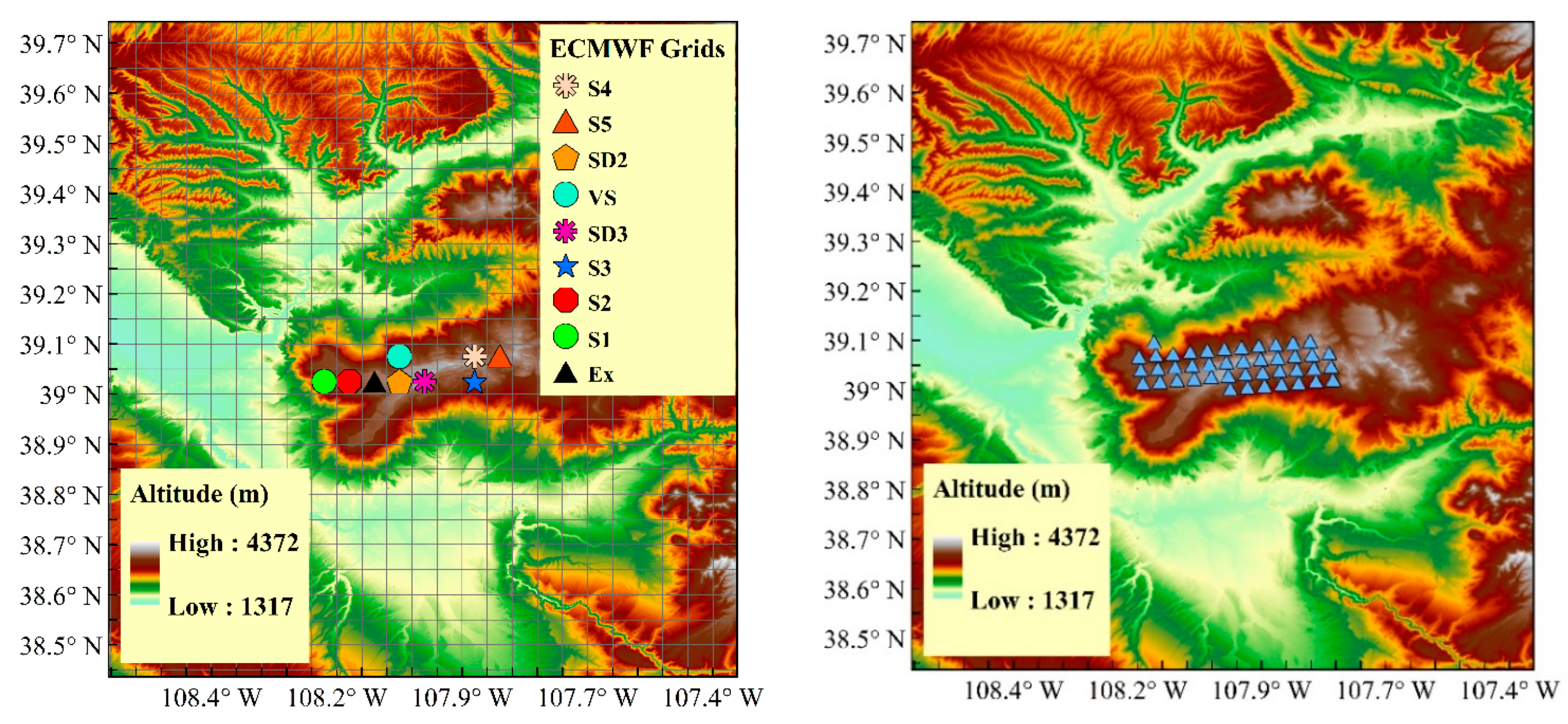
Figure 1. Topographic map of Grand Mesa with ECMWF grid cells (overlain grid on the left panel) and 43 grid points from the HRRR model (triangles on the right panel). Snowpit locations from the SnowEx’17 field campaign are clustered into nine groups corresponding to individual ECMWF grid cells (~5 × 5 km2) marked on the left panel. Each cluster contains at least eight snowpits. Table S1 in Supplementary Information provides the central (latitude, longitude) coordinates for each grid. The coordinates of the HRRR grids are fully or partially within the corresponding ECMWF grid. ECMWF— European Center for Medium-Range Weather Forecasts. HRRR—High-Resolution Rapid Refresh NOAA model.
Remotesensing 12 03422 g001
Figure 2. Land-use and land-cover (LULC) map centered over Grand Mesa. The nine snowpit clusters (Table S1) corresponding to nine ECMWF grid cells marked in Figure 1 are also marked here using the naming convention indicated in the legend.
Remotesensing 12 03422 g002
Figure 3. Information flow diagram in the coupled MSHM/MEMLS framework. At a given time t, the MSHM simulates a snowpack consisting of a number of layers nlayers(t), and yields snowpack stratigraphy consisting of the vertical profile of layer thickness (hsnow), snow water content (hswe), liquid water content (LWC), density (ρs), temperature Ts including ground temperature T0, and snow correlation length Lc. At the surface of the snowpack, latent heat (LH), sensible heat (SH), net radiation (Rnet), and outmelt (OM) fluxes are also calculated. The snowpack stratigraphy and temperature profiles are passed onto MEMLS to simulate the vertical profiles of transmissivity t , volume reflectivity r, emissivity e, interface reflectivity s, and refracted angle θ b where j = i. Incoming electromagnetic radiation (not shown) hits the snowpack surface of roughness ms with incidence angle θ n (not shown). The MEMLS output is the brightness temperature. Tb,s, and backscattering coefficient σs at the surface for frequency f, horizontal and vertical polarization.
Remotesensing 12 03422 g003
Figure 4. Time series of Ensemble 5 SWE and snow depth predictions on February 17 at S2 (a,b), SD3 (c,d), and S5 (e,f). The blue dotted line is the Ensemble 5 mean. The green envelope identifies the minimum and the maximum values among all ensemble members. The yellow envelope delimits the 25th and 75th percentiles. The symbols represent the SnowEx’17 snowpit observations following the convention in Table S2.
Remotesensing 12 03422 g004
Figure 5. Evaluation of model bias at reference ECMWF grid points (Figure 1) during SnowEx’17 (Table S1). (a) Local bias calculated as the difference between the Ensemble 5 Member corresponding to the nearest HRRR grid and the average of SnowEx’17 snowpit measurements within each ECMWF reference grid point for the entire month of February. (b) Global bias is calculated as the difference between the Grand Mesa Ensemble 5 mean and the average snowpit measurements on the same day within each ECMWF reference grid point.
Remotesensing 12 03422 g005aRemotesensing 12 03422 g005b
Figure 6. Evaluation of predicted snow density (a,b) and temperature (c,d) profiles against measured snowpit profiles (circles). Left column: Ensemble 5 Member 13 (HRRR grid point closest to the SD3 ECMWF grid center, Figure S1a). Right column: Ensemble 5 Member 29 (HRRR grid point closest to the center of the S5 ECMWF grid, Figure S1a). The measured values are graphed at the measurement depth in the SnowEx’ 17 records. The model values are graphed at the mid-point of each layer. Time-series of simulated snowpack stratigraphy (number of layers and layer thickness) are available in Supplementary Information (Figure S7b,c).
Remotesensing 12 03422 g006
Figure 7. Evaluation of Ensemble 5 predictions of snow temperature (a,c,e, and g) and snow density (b,d,f, and h) against snowpit measurements within S2 on February 25. The continuous lines represent Ensemble 5 mean values at three distinct times close to the reported time of snowpit measurements. The green envelope represents the min–max range of ensemble predictions at each depth. Each row is associated with one of four distinct snowpits identified by different markers according to the convention in Table S2.
Remotesensing 12 03422 g007
Figure 8. Ensemble 5 predictions of the seasonal evolution of vertical snowpack profiles contoured by (a) temperature, (b) density, and (c) snow correlation length from 9/1/2016 through 6/30/2017.
Remotesensing 12 03422 g008
Figure 9. Spatial variability of H-pol brightness temperatures Tb (ad) and backscattering coefficients for C- (5.6 GHz, e,f) and Ka- (35.7 GHz, g,h) bands at 18:00 UTC (1 PM MST) across the Grand Mesa from Ensemble 2 (left column) and Ensemble 5 (right column) during February 2017. For each violin diagram, the white dot represents the median; the vertical black bar demarks the 25th and 75th percentiles; the upper and lower bounds represent the maximum and minimum values respectively; and finally, the colored contour is the density distribution.
Remotesensing 12 03422 g009
Figure 10. Temporal evolution of ensemble backscattering coefficient σ-HH and σ-HV at 5.6 GHz (a,b) and 1.3 GHz (c,d) contoured by Ensemble 5 SWE. The black line is the Ensemble 5 mean. Note the diurnal cycle of the sensitivity of the ensemble mean that it is dominant at 5.6 GHz, including for high SWE ensemble members.
Remotesensing 12 03422 g010
Figure 11. (a) Backscattering behavior of σ-VV at 5.6 GHz and snowpack properties along the west–east transect formed by Ensemble 5 Members 32–42 in Grand Mesa (see maps in Figure 1 and Figure S1). (b) Liquid water content in the top snow layer. (c) Temperature of the top snow layer. (d) Snowpack depth. MST-Mountain Standard Time = UTC-7.
Remotesensing 12 03422 g011
Figure 12. Temporal evolution of Ensemble 5 backscattering coefficients σ-HH and H-pol brightness temperatures at 5.6 GHz (a,b) and 1.3 GHz (c,d) contoured by correlation length of the snowpack top layer. The black line is the Ensemble 5 mean. The red box marks the overnight period from 2/10/2017 to 2/11/2017, followed by daytime hours. UTC = Mountain Standard Time + 7.
Remotesensing 12 03422 g012
Figure 13. Diurnal cycle of 5.6 GHz σ-HH and H-pol brightness temperatures contoured by SWE (a,b), and temperature (c,d) and liquid water content (LWC, e,f) of the top layer of the snowpack at S2 over the period 2/10–2/13 for EFF2. The ~10 dB range on 2/12 results from compounding nonlinear effects of modest sub-grid-scale spatial variability of snow depth (Figure S12) and mid-day temperatures above the freezing level that cause melting at the snowpack surface. UTC = Mountain Standard Time + 7.
Remotesensing 12 03422 g013
Figure 14. Diurnal cycle of brightness temperature Tb-H at 5.6 GHz (top row) and 1.3 GHz (bottom row) for all Ensemble 5 members, thus capturing the snowpack’s spatial variability across the Grand Mesa during the warm weather period 2/10–2/23 from left to right. Note snowpack disappearance for some ensemble members (SWE = 0) on 2/11 (e.g., Figure 11) and 2/12 due to melting. The high ambiguity (spatial variance) introduced by the local meteorology is apparent with multiple SWE values for each Tb at 5.6 GHz, particularly for intermediate and deep snow and during the daytime. The green arrow indicates the direction of Tb increase during nighttime cooling and refreezing of the snowpack; the dark blue arrow indicates Tb decrease during daytime warming with substantial surficial melting.
Remotesensing 12 03422 g014
Figure 15. Snowpack monitoring in Grand Mesa at 1.3 GHz HH-pol during the accumulation season, January-February 2017. (a) Heuristic linear relationship between snowpack accumulation and backscatter (R2 > 0.95) reflects the integration of variable weather conditions in January and February in the simulated snowpack. (b) SWE and backscatter increments, respectively ΔSWE and Δσ-HH, are calculated as the difference between today’s and yesterday’s values at 7 AM MST. MST- Mountain Standard Time = UTC-7.
Remotesensing 12 03422 g015
Figure 16. (a,b) Seasonal evolution of Ensemble 5 mean backscatter at 7 PM MST across the Grand Mesa throughout the snow season from 9/1/2016 through 6/30/2017. (c,d) Seasonal evolution of Ensemble 5 mean brightness temperatures at 7 PM MST across the Grand Mesa throughout the snow season from 9/1/2016 through 6/30/2017. The microwave behavior is similar for all polarizations. MST- Mountain Standard Time = UTC-7.
Remotesensing 12 03422 g016
Figure 17. Conceptual synthesis of microwave hysteresis: (a) Synthesis of seasonal snowpack backscatter behavior as a function of SWE exhibiting hysteresis between accumulation and melt phases at L- and C-band (e.g., 1.3 and 5.6 GHz). Hysteresis is not present at Ku-band (e.g., 13.5 GHz) and higher frequencies; (b) synthesis of seasonal brightness behavior as a function of SWE exhibiting hysteresis between accumulation and melt phases at L- and C-bands.
Remotesensing 12 03422 g017
Figure 18. (a) Synthesis of scaling behavior of Sentinel-1 C-Band SAR backscatter in the Grand Mesa during 2017 from [9] that can be used to estimate the snowpack backscatter over different backgrounds (Green-grassland; Pink- forest; Blue-Mixed grass and forest) backscatter simulated in this study (orange circle) and at different spatial resolutions using fractal downscaling [42]. (b) Contrast between scaling behavior for dry and wet snow conditions. The spectra for different land-covers were separated by and arbitrary δ to facilitate visualization.
Remotesensing 12 03422 g018
Table 1. Summary description of ensemble forecast family 1 (EFF1) design. Grand Mesa ensembles are produced using 9 ECMWF and 43 HRRR distinct forcing time-series. Data are available at https://barros-group.cee.duke.edu/data-access.
Ensemble012345
Air temperature (K)ECMWFHRRRHRRRHRRRHRRRHRRR
Snowfall rate (kg/m2/s)ECMWFECMWFHRRRHRRRHRRRHRRR
Rainfall rate (kg/m2/s)ECMWFECMWFHRRRHRRRHRRRHRRR
Air pressure (Pa)HRRRHRRRHRRRHRRRHRRRHRRR
Incoming shortwave radiation (W/m2)ECMWFECMWFECMWFECMWFECMWFHRRR
Incoming longwave radiation (W/m2)ECMWFECMWFECMWFECMWFECMWFHRRR
AlbedoNLDASNLDASNLDASNLDASNLDASNLDAS
Windspeed (m/s)ECMWFECMWFECMWFHRRRHRRRHRRR
Specific humidity (kg/kg)ECMWFECMWFECMWFECMWFHRRRHRRR
Ensemble Size38738738738738743
Table 2. Parameters set for active and passive microwave remote sensing of snow in MEMLS. The scattering coefficient refers to the specific parameterization of the 6-flux scattering coefficients, and 11 was proved to be the best [35]. * Parameter estimated from Sentinel-1 5.6 GHz measurements.
Frequency (GHz)1.3, 5.6, 13.5, and 35.7 GHz
Incidence angle (º)50
Snow-ground reflectivity, h-pol0
Snow-ground reflectivity, v-pol0
Specular part of snow-ground reflectivity, h-pol0
Specular part of snow-ground reflectivity, v-pol0
Sky brightness temperature (K)0
Type of scattering coefficient11
Mean slope of snow surface undulations0.1
Cross polarization fraction *0.2
Snow salinity (parts per thousand)0
Publisher’s Note: MDPI stays neutral with regard to jurisdictional claims in published maps and institutional affiliations.