Article

Modeling Spatial Flood using Novel Ensemble Artificial Intelligence Approaches in Northern Iran

1
Department of Geomorphology, Tarbiat Modares University, Tehran 14117-13116, Iran
2
Department of Geography, University of Gour Banga, Malda 732103, West Bengal
3
Department of Geography, Chandidas Mahavidyalaya, Birbhum 731215, India
4
Department of Geoinformatics–Z_GIS, University of Salzburg, 5020 Salzburg, Austria
5
College of Geology & Environment, Xi’an University of Science and Technology, Xi’an 710054, China
6
Key Laboratory of Coal Resources Exploration and Comprehensive Utilization, Ministry of Land and Resources, Xi’an 710021, China
7
Shaanxi Provincial Key Laboratory of Geological Support for Coal Green Exploitation, Xi’an 710054, China
8
Faculty of Information Technology, Hanoi University of Mining and Geology, No. 18 Pho Vien, Duc Thang, Bac Tu Liem, Hanoi 10000, Vietnam
9
Future Technology Research Center, College of Future, National Yunlin University of Science and Technology, 123 University Road, Section 3, Douliou, Yunlin 64002, Taiwan
10
Institute of Research and Development, Duy Tan University, Da Nang 550000, Vietnam
*
Author to whom correspondence should be addressed.
Remote Sens. 2020, 12(20), 3423; https://doi.org/10.3390/rs12203423
Submission received: 7 August 2020 / Revised: 11 October 2020 / Accepted: 16 October 2020 / Published: 18 October 2020
(This article belongs to the Special Issue Urban Flooding Monitoring Using Remote Sensing)

Abstract

:
The uncertainty of flash flood makes them highly difficult to predict through conventional models. The physical hydrologic models of flash flood prediction of any large area is very difficult to compute as it requires lot of data and time. Therefore remote sensing data based models (from statistical to machine learning) have become highly popular due to open data access and lesser prediction times. There is a continuous effort to improve the prediction accuracy of these models through introducing new methods. This study is focused on flash flood modeling through novel hybrid machine learning models, which can improve the prediction accuracy. The hybrid machine learning ensemble approaches that combine the three meta-classifiers (Real AdaBoost, Random Subspace, and MultiBoosting) with J48 (a tree-based algorithm that can be used to evaluate the behavior of the attribute vector for any defined number of instances) were used in the Gorganroud River Basin of Iran to assess flood susceptibility (FS). A total of 426 flood positions as dependent variables and a total of 14 flood conditioning factors (FCFs) as independent variables were used to model the FS. Several threshold-dependent and independent statistical tests were applied to verify the performance and predictive capability of these machine learning models, such as the receiver operating characteristic (ROC) curve of the success rate curve (SRC) and prediction rate curve (PRC), efficiency (E), root-mean square-error (RMSE), and true skill statistics (TSS). The valuation of the FCFs was done using AdaBoost, frequency ratio (FR), and Boosted Regression Tree (BRT) models. In the flooding of the study area, altitude, land use/land cover (LU/LC), distance to stream, normalized differential vegetation index (NDVI), and rainfall played important roles. The Random Subspace J48 (RSJ48) ensemble method with an area under the curve (AUC) of 0.931 (SRC), 0.951 (PRC), E of 0.89, sensitivity of 0.87, and TSS of 0.78, has become the most effective ensemble in predicting the FS. The FR technique also showed good performance and reliability for all models. Map removal sensitivity analysis (MRSA) revealed that the FS maps have the highest sensitivity to elevation. Based on the findings of the validation methods, the FS maps prepared using the machine learning ensemble techniques have high robustness and can be used to advise flood management initiatives in flood-prone areas.

Graphical Abstract

1. Introduction

Floods and earthquakes are the most common and unpredictable natural events that cause damage to communities by affecting lives and property [1]), and determine the basin landforms [2]. Flash flooding is more disastrous than any other type of flooding because of its very short lag time [3,4]. Flash floods occur suddenly in any region and, thus, it appears to be very difficult to predict such events [5]. Moreover, flash flood depends on volume of run-off, the associated run-off velocity and infiltration by soil and its impact varies from region-to-region based on its geo-physical background [5]. Thus, to identify the probable regions of flash flood accurately is quite difficult. The increase in frequency of such devastating flood events in many parts of the world is mainly driven by climate change and large total rainfall within short time periods [6,7,8]. It is also quite surprising that more than 90% of the loss of lives and properties in Asia is due to flooding rather than other natural or/and man-induced disasters [9,10]. Between 1988 and 2011, natural events caused the death of 390,000 people worldwide, of which 58% was due to flooding [1]. Since complete mitigation of floods and other natural disasters is not possible, reducing the impacts of floods is crucial for livelihoods and sustainable development. That is why flood susceptibility modeling helps to identify the flood prone zones within a vast territory, which becomes helpful for planners and decision-makers for flood management [11]. Thus, ultimately identifying flood-prone zones and mapping these areas in detail can help planners reduce the detrimental impacts. This is an important contribution to achieving the United Nations sustainable development goals and to effectively resolve the problem of the neutrality of land degradation [12] in arid and semi-arid lands in which floods, degradation of land, drought, and desertification endanger people and their natural resources [13,14].
In Iran, floods are one of the most devastating natural disasters, resulting in an almost $3.6 billion loss in Iran [15]. A variety of factors, such as rainfall change and geophysical conditions are believed to be responsible for the rise in the number of flood events causing the loss of life and property [16]. In the last six decades, in Iran, there has been 3700 flood incidents, the most widely affected northern Iran [17]. More specifically, the Gorganroud River Basin in Iran is well-known for its large number of floods, with over 120 recorded floods between 1991 and 2012 [18].
The suitability of a method for flood susceptibility (FS) assessment depends on the capability of this method, with respect to flood conditioning factors (FCFs) used in the modeling. The selection of factors is, therefore, the first and most important step, and is mainly based on previous flood studies. The next task is to determine the order of importance of these flood occurrence factors and apply the best methods to identify and predict the flood hazard zones precisely. There are many physically-based models for predicting hydrological events. Numerous researches, however, indicate that there is a short-term predictive potential difference in current physical models [19,20,21,22,23,24,25]. Consequently, physically-based models do not provide reliable quantitative flood predictions with the help of a limited amount of data, and these models accumulate uncertainty errors in the modeling results [26,27,28]. These shortcomings promote the use of machine learning (ML) models. Soft computing methods are now becoming very popular due to their capability for dealing with a large number of datasets of varying nature, and for generating highly accurate results. These methods include logistic regression [11,29,30,31], neuro-fuzzy inference systems [32,33,34], decision trees [30], support vector machines (SVMs) [31,32,33,34,35], evidential belief functions [36,37], artificial neural networks (ANNs) [38], analytical hierarchy process and fuzzy logic [39,40,41,42,43], frequency ratio [11,30,31,44,45], conditional probability, certainty factor and Shannon entropy [10], Technique for Order of Preference by Similarity to Ideal Solution (TOPSIS), and VIseKriterijumska Optimizacija I Kompromisno Resenje (VIKOR) [37].
Several ML algorithms were introduced and used for various hazard-mapping in the current decade [46,47,48,49]. Here, the hybrid ensemble methods are more capable of performing reliable predictive analysis [50]. Ensemble techniques, such as Bagging and Boosting, are widely used for classification problems where multiple independent categorical variables are simultaneously used to address one issue. These techniques are now emerging in the field of spatial analysis where the ensemble models are used in landslide hazard mapping [32,51,52,53] and groundwater potential analysis [54,55], but, so far, have rarely been used to model flood hazards [56,57]. The Real AdaBoost can obtain a strong classifier using fewer decision trees [58]. It combines the AdaBoost with a real-valued classifier; therefore, it gives a more accurate result compared to the AdaBoost model. The key benefit of the approach of Random Subspace is that it uses its samples of different spatial features to achieve sub-classification differences and provide better results [59,60,61,62]. MultiBoosting can generate a decision tree with a lower error than both AdaBoost and Wagging [63,64]. Instead, Real AdaBoosting, MultiBoosting, Random Subspace and J48 are widely used in other sectors, such as banking and finance. Accordingly, in the work reported herein, we applied and tested ensemble methods combining meta-classifiers (Real AdaBoosting, MultiBoosting, and Random Subspace) with a tree-based algorithm (i.e., J48) as novel approaches. In doing so, we tested the new approaches for flood prediction and hazard zoning in the Gorganroud River Basin, in northern Iran. More specifically, we evaluated the contribution of a range of independent factors on flood susceptibility using the FR method. The accuracy of the models were assessed using the efficiency, sensitivity, root-mean square-error (RMSE), and receiver operating characteristics (ROC) technique.
The principal aim of the work discussed in this paper is to evaluate flood susceptibility (FS) model capacity, in particular, the hybrid machine learning ensemble approaches using the Gorganroud River Basin, Iran, as a case study. This will bring information to understand, forecast, and prevent flash floods.

2. Materials and Methods

2.1. Description of the Study Area

Located in the Golestan Province in northern Iran, the Gorganroud River Basin stretches between latitudes 36°25′to 38°15′N and longitudes 56°26′ to 54°10′ (Figure 1). This basin spans an area of 11,290 km2, and falls into the Caspian Sea from the eastern Alborz Mountains. The height varies in the western zone (Caspian Sea) from −96 m above sea level (a.s.l). to 3669 m a.s.l. in the southern regions. The estimated annual temperature and precipitation are 17.8 °C and 500 mm, respectively [65]. The main climate types in the study area are semi-arid in the central part, Mediterranean in the northern areas, semi-humid in the south, and humid in the northeastern and northwestern regions. Based on the National Cartographic Centre and Geological Survey of Iran [66], lithological formations are also complex, but can be classified into four major age classes, consisting of Cenozoic, Mesozoic, Paleozoic, and Proterozoic. Agriculture, bare land, dry farmland, timber, rangeland, orchard, residential, water/wetland, and woodland are the nine major land use/land cover (LU/LC) types found in the study basin. Agriculture, woodland, and rangelands occupy much of the watershed. In the study area, seven types of soil have been described: Entisols, Inceptisols, Salt Flats, Alfisols, Aridisols, Inceptisols, and Mollisols, with spatially dominant Mollisols. Slopes in the watershed range from 0° to 79°, with most of the region (61.24%) having low slope angles (<14.2°). Due to extensive and unplanned land-use changes, and especially deforestation and urbanization, combined with heavy rainfall, this study area is recognized as one of the flood susceptible watersheds in Iran [18]. According to available evidence, between 1991 and 2019 more than 120 major and minor floods occurred in the basin [18]. For instance, the Gorganroud river flow reached 3020 cubic meters per second during the flood on 11 August 2001, and the river widened from 10 m to 400 m. This flood has caused over 500 deaths and is, thus, considered to be the most destructive flood in Iranian history [17]. Another example is a flood that occurred on 17 March 2019, during which, along with 12,000 houses, facilities, agricultural land, and gardens, most of the towns, including Aqqala and Gomishan, and at least 70 villages, were affected [67]. Given such devastating impacts arising from flooding, identifying the most susceptible areas in this flood prone region is crucial for targeting management for reducing flood damage.

2.2. Methodology

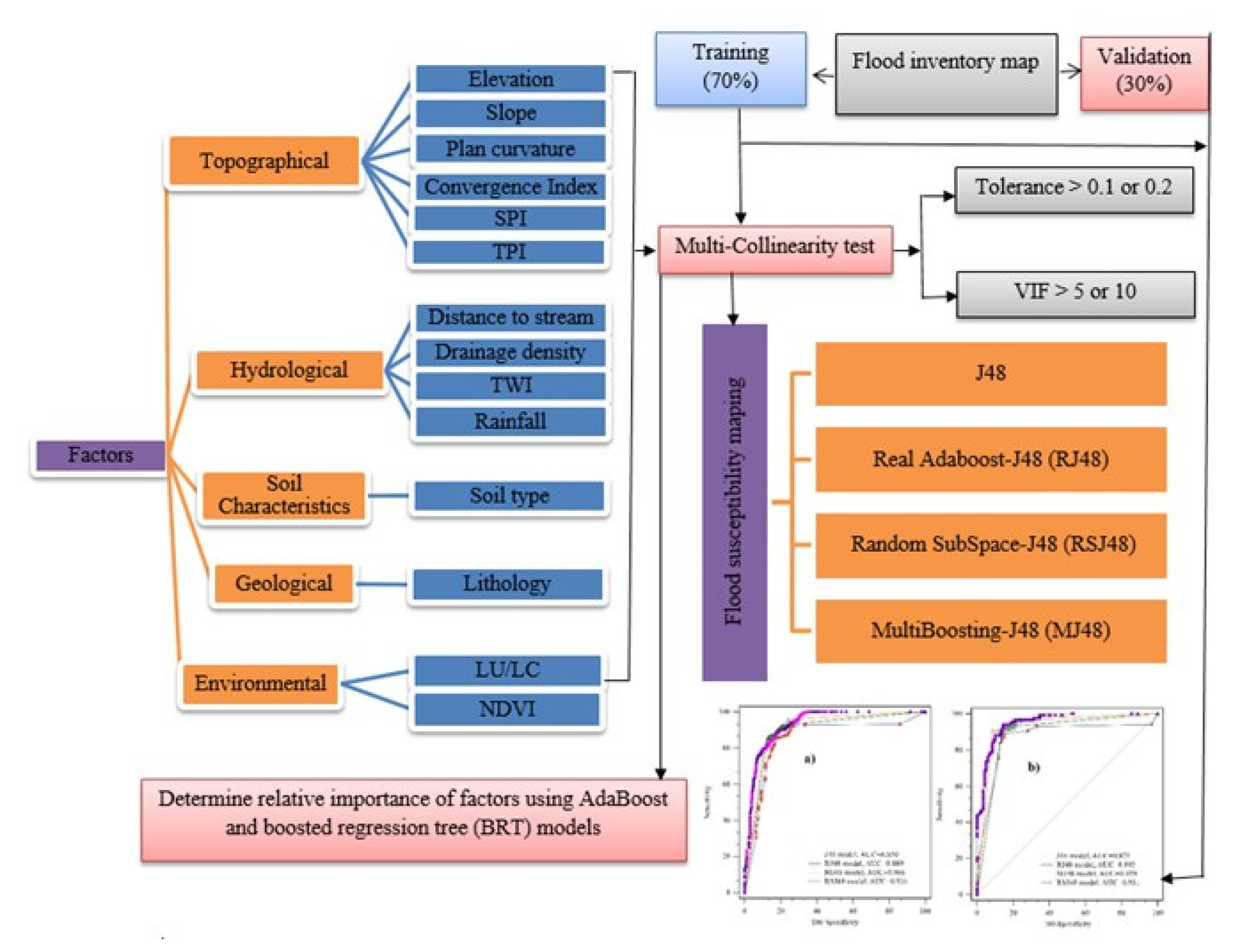
Flood susceptibility maps were prepared as part of this study using three novel ensemble ML algorithms. Using a number of main steps, the analysis was carried out. Firstly, two kinds of data, i.e., flood incidence and flood conditioning factors (FCFs), were gathered. Secondly, the flood inventory map and thematic layers of the FCFs were prepared (elevation, slope, curvature of the plan, topographic position index (TPI), topographic wetness index (TWI), convergence index (CI), stream power index (SPI), drainage density (DD), stream distance, precipitation, lithology, land use/land cover (LU/LC), normalized difference vegetation index (NDVI), and soil type). Third, 426 flood locations were reported, 70% of which were considered to prepare FS models, and 30% of which were used to validate models produced using training datasets. In step four, the tolerance was applied and the variance inflation factor (VIF) multicollinearity was tested among the selected FCFs. VIF estimates the multicollinearity problem among the independent factors, and if it is present, then that factor should not be used for modeling. In step five, the contribution of the factors was analyzed using the frequency ratio (FR), boosted regression tree (BRT), and AdaBoost. For step six, in order to produce the flood susceptibility map (FSM), training data was first applied to predict the spatial flood susceptibility (FS) using the base classifier of J48. Then, FSMs were prepared using meta-classifiers (i.e., Real AdaBoost, Random Subspace, and MultiBoosting) ensemble models (Real AdaBoost J48, Random Subspace J48, and MultiBoosting J48). Finally, we validated the FSMs generated by the ensemble models using the ROC curve, efficiency, accuracy, and true skill statistics (TSS), and analyzed the sensitivity of the individual flood conditioning factors to the four models. Figure 2 summarizes the key steps in our methods. J48, Real AdaBoost J48, Random Subspace J48, and MultiBoosting J48 models were run in R studio programming software using the CRAN R Weka, party, regRSM packages. Finally, the layouts of the flood susceptibility maps were prepared using ArcGIS software.

2.3. Database

2.3.1. Flood Inventory Map (FIM)

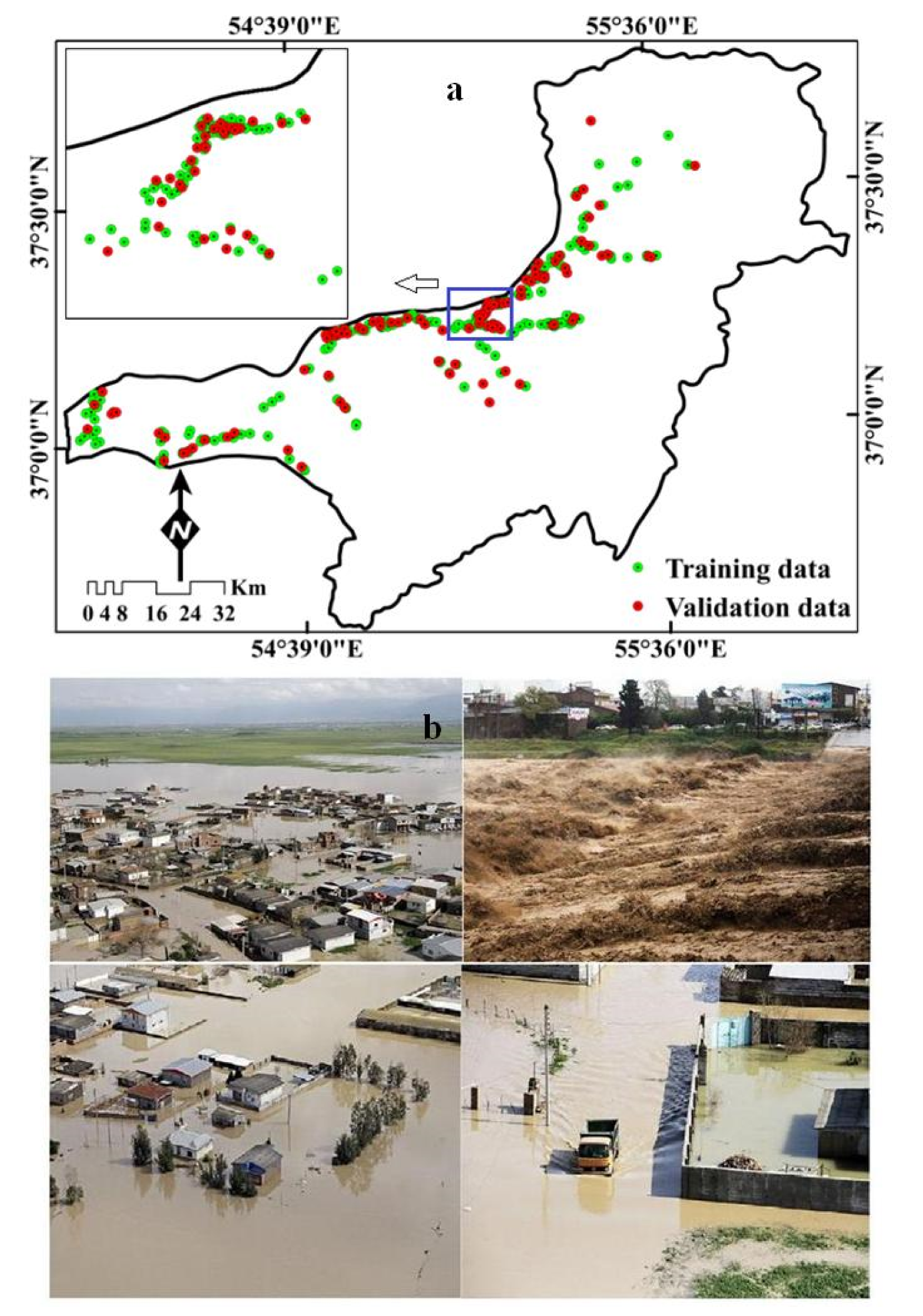
The flood location was regarded as the dependent variable for the calibration of the FSMs, and the effective FCFs were regarded as the independent variables. Using the dependent and independent variable data, the FSMs were prepared based on the J48 and ensemble models. It is necessary to prepare a FIM for the spatial flood probability prediction [10,36]. In previous works, several sources were used for preparing the FIM, such as governmental sources, newspaper articles, field surveys, etc. Modified Normalized Difference Water Index (MDNWI) derived from the Sentinel-2 satellite images through the Google Earth Engine can be used for preparing the FIM [56]. In this study, for the period 2001–2019, we used records from the Ministry of Iranian Water source, investigation documents on disaster management in the Golestan Province, and, three times, field surveys were carried out (on 8 February 2018; 2 April 2019; and 21 May 2019) in the randomly selected points to construct the flood inventory map. Flood points were selected randomly among the flood sites, having the flood frequency of one flood per year. We listed 426 flood sites in the research region (Figure 3), which we randomly divided into two datasets, i.e., a training dataset (70%) and a test data set (30%). We also selected the same amount of non-flood sites, randomly, for training as well as validating the models.

2.3.2. Generating Flood Conditioning Factors (FCFs)

Many factors control the flood susceptibility (FS) of an area, but there are no standard criteria for selecting the FCFs to depict the spatial FS. We initially selected 16 FCFs on the basis of previous literature, but eventually selected six topographical factors (elevation, slope, plan curvature, SPI TPI and CI), four hydrological factors (TWI, DD, stream distance, and rainfall), two environmental factors (LU/LC and NDVI), as well as lithology and soil type after multicollinearity analysis for FS modeling [10,35]. A geological map from the Geological Survey of Iran, rainfall data from the Islamic Republic of Iran Metrological Organization, Landsat 8 Operational Land Imager (OLI) from the United States Geological Survey (USGS) (https:/earthexplorer.usgs.gov/), Phased Array type L-band Synthetic Aperture Radar Digital Elevation Model (PALSAR DEM) of 12.5 × 12.5 m resolution from the Alaska satellite facility, and soil from Mazandaran Agricultural and Natural Resources Research Centre were obtained for the preparation of the thematic FCF layers. PALSAR DEM is considered the most accurate DEM available free of charge [68]. The level of vertical accuracy is most important for the mapping the spatial flood susceptibility. Just like Gesch et al. [69], it was done to calculate the uncertainty in the DEM comparison between Advanced Land Observing Satellite (ALOS) DEM elevations and those of the ground control points (GCPs) [69]. In this analysis, ALOS DEM was used with a vertical precision of 0.3 m.
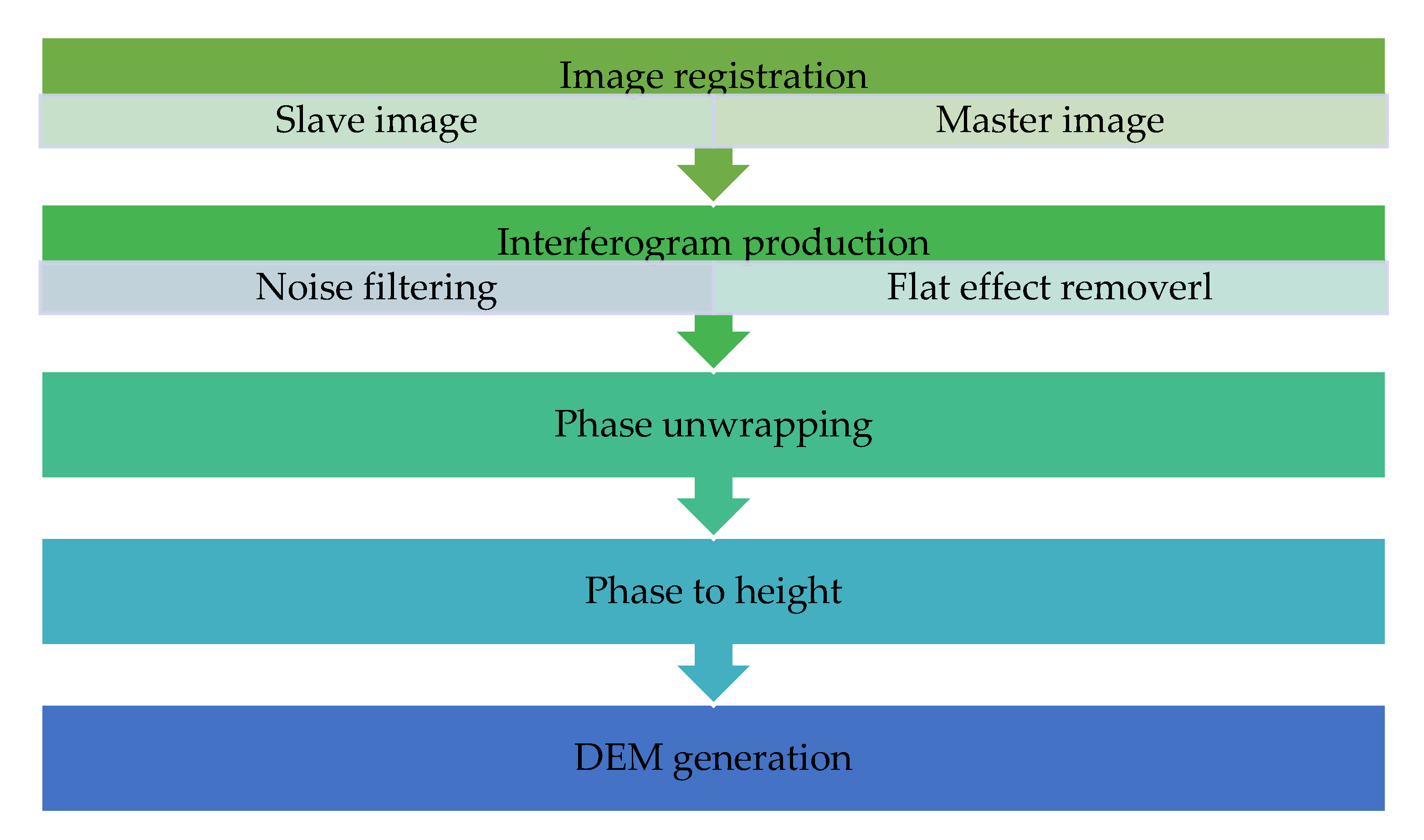
For geomorphological research and modeling natural disasters, a reliable topographical data source is essential [70]. The Interferometric synthetic aperture radar (InSAR) system and the ALOS–PALSAR data (slave image: 12 August 2009, and master image: 18 September 2012) were used in our research to construct a high precision DEM. The most critical phases in the generation of InSAR DEM include phase estimation and the transformation from phase to height [71]. In Figure 4, the steps for generating a DEM using InSAR are presented. PALSAR sensor images for the study area were downloaded (www.nasa.gov) to provide a DEM of the region. For the entire study area, the PALSAR DEM was generated using the Mosaicing method incorporated in ENVI5.1 software. To boost the accuracy and reduce the errors of the DEM derived from PALSAR, filters were used. The right filters were chosen using experiments, defects, and recommendations from other researchers [72]. A basic filter (smooth 2 × 2) was used to eliminate errors and enhance detection precision and the hydrological calculation precision was improved with the Fill Sinks filter.
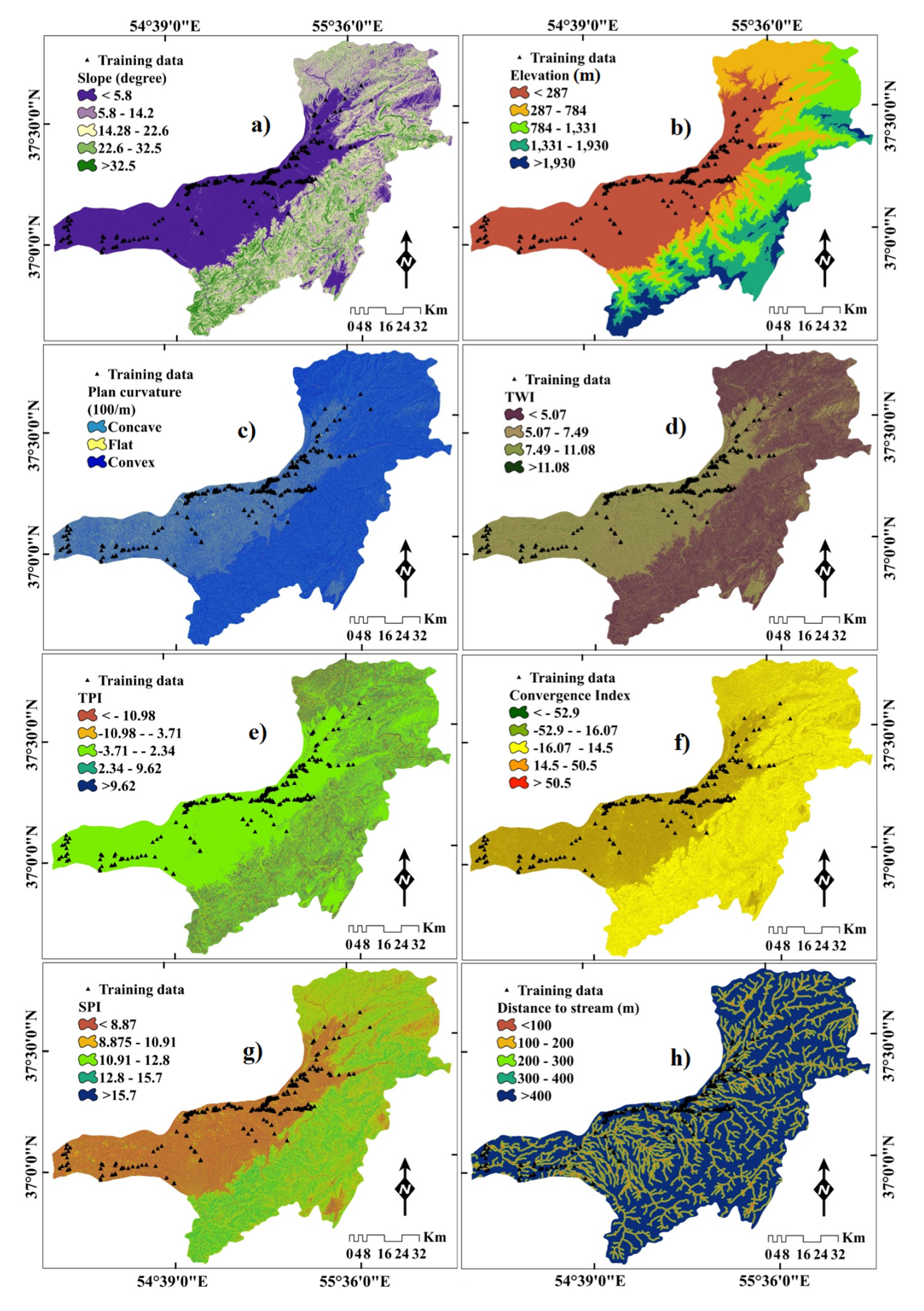
Slope: flooding is specifically related to the gradient of slopes [73,74,75]. The surface slope of the area (Figure 5a) is an important factor influencing the frequency of flooding, since there is very little opportunity for rainwater to penetrate steep hills and much more opportunity for rainwater to penetrate plain and gently sloping land [30]. The slope determines not only the velocity of the flow, but also the intensity and volume of run-off. Steeper slopes are more vulnerable to flash floods, but gentle slopes are more likely to experience longer duration flooding. Ultimately, the combination of steep slopes in the upper part of the watershed and gentle slopes in the lower portions magnifies the local flood hazard. The stagnation of water for longer periods mostly affects the flat regions and the most devastating floods also occur in the lower sloping areas. Therefore, the slope of the study area significantly affects the intensity and duration of any flood event.
Elevation: among the different FCFs (Figure 5b), there is a reciprocal relationship between flooding and elevation [30]. The areas at a low altitude are more susceptible to floods than the higher altitude regions [76]. In reality, flooding in high elevation areas is almost impossible [77]. The height of the basin varies from 64 to 3686 m, suggesting the existence of low-lying flat plains as well as hilly terrain and mountains, while the bulk of the sample region is flat plains (Figure 5b).
Plan curvature: the curvature of the plan is a morphological element regulating the vulnerability of flooding by the controlling of water flow on a region’s surface [44]. The plan curvature in the region analyzed ranges from −25.79 to 31.61 (Figure 5c). The area’s plan curvature is categorized into three concave, flat, and convex types, whereby concave areas preserve water and convex areas induce runoff. Interestingly, both concave and convex areas make up similar proportions of the study basin (45% each), which indicates that the basin is susceptible to both high run-off and flood retention.
Topographic wetness index (TWI): introduced by Beven and Kirkby [78], the TWI defines the spatial wetness status in the basin, which influences the susceptibility to flooding [28]. The TWI represents the effect of topography at every point in the catchment on the output of runoff and the volume of flow accumulation [79]. The TWI is calculated from the following Equation (1):
TWI = In ( A S / tan β )
where, in respect to per unit contour length (m2/m), A S represents the upslope area and β is the slope gradient (degrees). The TWI in this basin ranges from 0.55 and 24.09 (Figure 5d).
Topographic positioning index (TPI): TPI is defined as the altitudinal difference within a specified radius (R) between the central point (Z0) and the average elevation ( Z ¯ ) around it [80,81]. Utilizing Equations (2) and (3), the TPI is measured.
TPI = Z 0 Z ¯
Z ¯ = 1 n R i R Z i
The TPI value relies on the unit (R) of the landscape. A small R reveals small valleys and ridges [82]. TPI ranges from −142.59 to 152.29 within the area of study (Figure 5e).
Convergence index (CI): the CI is a major terrain element showing the relief structure of the study region as a series of channels (convergent areas) and ridges (divergent areas). It was posed by Kiss [83]. The CI is calculated using the following Equation (4):
C I = ( 1 8 i = 1 8 θ i ) 90 0
where: the average angle is shown by θi between the direction of the neighboring cells and the central cell location. The value of CI varies between −100 and +100 in the study region (Figure 5f).
Stream power index (SPI): the SPI demonstrates the erosive capacity of surface running water [84], which has been demonstrated to affect flood vulnerability [85]. DEM was used to derive the SPI using the following Equation (5):
SPI = A s × tan β
where: the upstream region is As, and the gradient is β. The spatial distribution of the SPI ranges from 6.27 to 26.35 (Figure 5g) in the basin.
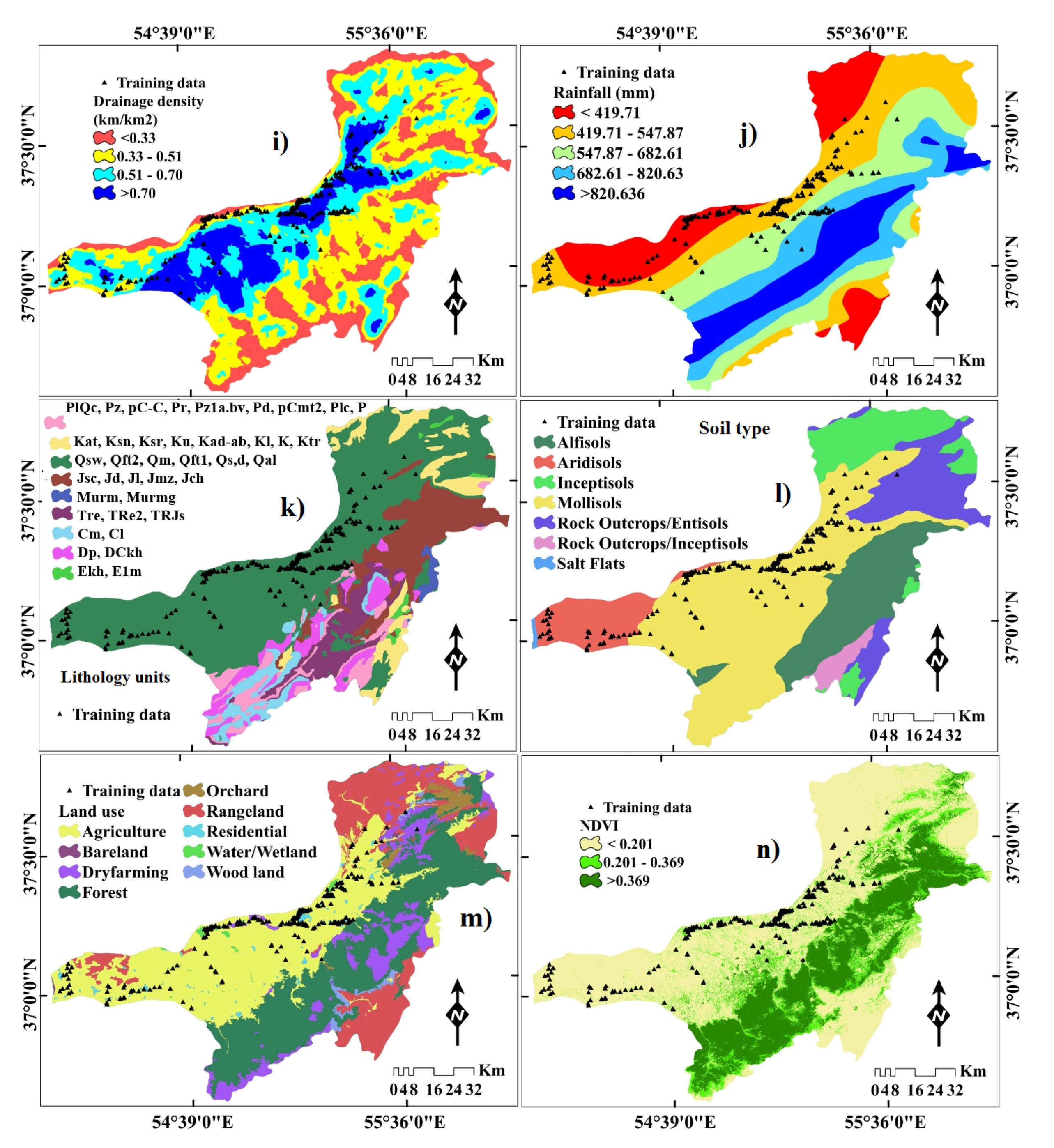
Distance to stream: a method for extracting stream buffer in ArcGIS was applied is the Euclidean distance buffer (Figure 5h). Areas along the main river are more susceptible to floods, but less susceptible to remote areas [86].
Drainage density (DD): drainage density (Figure 5i) is able to exert good influence over the frequency of floods and is calculated from the DEM using the ArcGIS line density tool [87]. This research has identified four DD groups (e.g., <0.33, 0.33–0.51, 0.51–0.7 and >0.7).
Rainfall: for the purposes of plotting average rainfall thirty years (1986 through 2016) rainfall data were obtained for 44 meteorological stations (Figure 1). The Wahba first suggested thin plate spline process is an effective and efficient system of interpolating. In order to prepare the raster layer of rainfall data collected from different weather stations, a modified orthogonal least-square plate spline (TPS-M) was used. This technique is more reliable than the traditional method of interpolation. The works of Boer et al. [88] offered detailed explanations for the technique. Rainfall plays a central role in flood occurrence within a region, as it is the source of water in the channels as well as in the ground [89]. We defined five rainfall categories for the purpose of this study, namely <419.71 mm, 419.71–547.87 mm, 547.87–682.61 mm, 682.61–820.63 mm, and >820.636 mm.
Lithology and soil type: lithological and soil maps are of considerable significance when assessing flood-prone areas as the characteristics of the soil, such as density, degree of permeability, composition, and form of substrate directly influence the drainage cycle. The lithology and soil of a region regulate flooding by regulating erosion and infiltration in a watershed [85]. The lithological and soil maps (Figure 5k and 5l for the study area were drawn up on the basis of an available geological map (scale: 100,000) and a soil map (1:250,000) from a Research Centre for Agricultural and Natural Resources in Mazandaran. Nine lithological units (Supplementary Table S1) and seven soil classes, (Entisols, Inceptisols, Salt Flats, Alfisols, Aridisols, Inceptisols, and Mollisols) were identified.
LU/LC and NDVI: Landsat 8 OLI images were used for producing the LU/LC and NDVI maps (Figure 5m,n) in ArcGIS. Before preparing the LU/LC and NDVI, the satellite images are pre-processed through atmospheric and radiometric correction. Classes of LU/LC with bare land and concrete surfaces increase land flow, while dense forest and vegetation limit overland flows [26]. Moreover, 632 ground control points (GPs) were identified to test the classification accuracy of the LU/LC map. Out of the 632 GCPs 190, 239, 6, 10, 4, 56, 116, 8, and 3 GCPs were taken for forest cover, agriculture class, residential class, orchard class, bare land class, dry farming, rangeland, wood land, and water/wetland classes, respectively. Kappa coefficient was calculated using the Equation (6) [90]. The average precision of the LU/LC map was reasonable (Kappa coefficient = 0.972). Nine LU/LC categories were created for the study basin. From the Landsat 8 OLI, NDVI was calculated. For calculating the NDVI, band 4 and band 3 were used. The value above zero (towards +1) indicates the vegetation and the value below zero (towards −1) indicates the water body of the region. Three NDVI categories were defined, (i.e., <0.201, 0.201–0.369 and >0.369) to represent vegetation density. An NDVI value of >0 indicates the presence of vegetation and with increasing values, the probability of it being a forest increases.
K = { N i = 1 r ( X i i ) N i = 1 r ( X i + · X + i ) } N 2 i = 1 r ( X i + · X + i )

2.4. Multicollinearity Test of Effective Factors

Pradhan [91] reported a standard measure for detecting collinear variables among the factors used in probability modeling. Multicollinearity is a condition in mathematics where one predictor variable can be predicted linearly, based on the others, with a large degree of accuracy in a multiple regression model. It can identify the independent variables that can be used further in the model with the help of variance inflation factors (VIF) [92,93,94]. A VIF value greater than 5 suggests a concern with multicollinearity [95,96]. If the test identifies any collinear variable, then it should not be used for predictive modeling. In this study, fourteen independent variables were used for flood susceptibility analysis based on previous flood-related research, meaning that assessment of multicollinearity was important. The VIF was determined using the following Equation (7) among certain variables:
V I F = 1 T o l e r a n c e

2.5. Analysis of the Relationship between FCFs and Flood Occurrences Using the Frequency Ratio (FR) Model

The FR was used to determine the relation between FCFs and the frequency of floods. For a given class of variables, the FR can be defined as the ratio of the likelihood of flood to non-flood, which can be calculated in terms of the percentage share of flood pixels divided by the domain type pixel [97]. The FR values represent the importance of the class variables in terms of flood probability:
FR = Li / Ci L / C
where: Li is flood cells in the ith category, Ci is the total cells in the ith category, L is total flood cells, and C is the total cells. An FR value >1 shows the greater flood cell concentration in a given segment as compared to the total data layer. On the other side, if a certain category’s value is below 1, this suggests a small concentration of flood cells in the data layer.

2.6. Flood Susceptibility Spatial Modeling using Machine Learning Ensemble Methods

2.6.1. J48 Decision Tree

J48 is a decision tree algorithm that can be used to determine the attribute vector’s behavior for any given number of instances [98]. The algorithm creates the rules for target variable prediction, and with the help of tree classification and the data distribution, can also be simply conceptualized [95]. The add-on features in J48 include its ability to account for missing values, tree pruning, and setting rules. It is also able to generate data mining results with higher accuracy compared to other tree-based algorithms. For the generation of decision trees, this J48 ensemble model uses the C4.5 algorithm, which is very efficient in statistical classification [99]. It is an attribute selection method performed using input information and entropy equations from any types of data with class levels [100].

2.6.2. Real AdaBoost

Freund and Schapire [101] proposed this new ML ensemble model to make multiple weak classifiers into one strong classifier through the process of boosting. Training data subsets can easily be obtained from such ensemble models. The AdaBoost algorithm is based on the following mechanisms: firstly, a subset of the training samples is developed, and then the initial classification configuration is generated according to the same weighted factors. Secondly, all training dataset events are simulated in this fundamental model. The erroneous cases now weight more, while the correctly graded instances weigh the same. Thirdly, the weights are standardized for all training instances and a new subset is randomly generated to develop the next model classifier-based model. That is working continuously until it stops. Ultimately, we end up with a good classifier model owing to the weighted total of all the classifier-based models previously developed.
The Real AdaBoost is a modified and advanced form of the AdaBoost that can be used to obtain a strong classifier using fewer decision trees [58]. Friedman, Hastie, and Tibshirani [101] first introduced this ensemble method from a formal statistical perspective. Their work has shown that the Real AdaBoost removed the necessity of having a coefficient as the optimal coefficient—αj = 1 [58]. It combines the AdaBoost with a real-valued classifier or half of the weighted log odds predicted by the classifier; therefore, it gives a more accurate result compared to the AdaBoost model. In the final stage, the Real AdaBoost combines all the decision tree values into one value; hence, the model can be represented as a scorecard [101].

2.6.3. Random Subspace

The problem of over-fitting the training data for classification in decision trees with the highest accuracy can be overcome using Random Subspace [56]. This can be used to create a tree-based decision classifier that can preserve the maximum precision of training data coupled with increased generalization performance with increasing difficulty. Here, this ensemble method is quite similar to Bagging and trees are constructed in randomly selected subspaces [102,103,104,105]. Therefore, from the original training datasets, the subspaces were randomly chosen and through a combination of voting methods, the final result was generated from the subset of each classifier training dataset [106,107]. The key benefit of the approach of learning Random Subspace is that it uses its set of samples of varying spatial characteristics to achieve variations in sub-classification [59,60,61,62].

2.6.4. MultiBoosting

MultiBoost is an enhancement of the AdaBoost concept that uses the power of both AdaBoosting and Wagging to solve the issue of over-fitting [63,64]. MultiBoosting can generate a decision tree with a lower error than both AdaBoost and Wagging. It is also able to perform parallel executions, which makes it more advanced compared to AdaBoost. MultiBoosting uses a random bootstrap sampling approach to establish training subsets and allocate random weights to each subset [64]. Therefore, the step-by-step process of MultiBoosting is as follows. Firstly, using the training dataset, a set of training subsets is formed through random selection and replacement and then it is used to build the classifier-based model. Secondly, the weights are determined based on the overall accuracy of the classifier-based model. Thirdly, the new subsets are developed on the basis of continuous sampling and instance weightings to train the new classifier-based models from which the result is generated in the form of classifiers.

2.7. Model Validation Techniques

Validation of the results generated from flood hazard susceptibility maps (J48, MultiBoosting J48 (MJ48), real AdaBoost J48 (RJ48), and Random Subspace J48 (RSJ48)) is an essential part of the work required to obtain a meaningful conclusion. To quantitatively validate each model, the receiver operating characteristic (ROC) curve was applied [30,108]. For various types of predictive models, ROC is a widely known validation method [109]. The ROC curve defines the reliability of the model by the AUC (area under curve). The AUC values range between 0.5 and 1 where 0.5 reveals that the model cannot estimate the susceptibility to flooding, and 1 implies a good forecast [110]. Of all the flood inventory points, flood susceptibility index values were binarized considering the threshold flood probability index values, which is “the optimal point on the ROC curve closest to the point (0, 1)” using the ‘Optimal Cutpoints’ package in R [111]. For both training and testing data sets, the ROC curve was used to test the susceptibility maps for flood hazards. The ROC curves of training datasets are called success rate curves for existing flood hazards, whereas the ROC curves of validation datasets are termed prediction rate curves for future flood hazard probabilities. The ROC was equipped to equate the true positive (TP) values with the false positives (FP) at different thresholds. The true positive rate (TPR) is seen as precision and the false positive rate (FPR) as the specificity, drop, or probability of an inaccurate calculation. A higher TPR is more reliable and a higher FPR is the representation of model prediction errors. The equations for TPR and FPR are as follows:
TPR = TP TP + FN
FPR = FP FP + TN
A U C = ( T P + T N ) / ( P + N )
where: TN, FP, TP, and FN are the true negative, false positive, true positive, and false negative respectively [112]. The scale of TPR ranges from 0 to 1, whereby the categorical subdivisions are as follows, Excellent (0.9–1), very good (0.8–0.9), good (0.7–0.8), moderate (0.6–0.7), and weak (0.5–0.6) [107]. RMSE (Equation (10)) was used to determine the difference between actual and expected flood results. Low values of RMSE indicate better models [106,113].
R M S E = 1 n i = 1 n ( X p r e d i c t e d X a c t u a l ) 2
In addition, two threshold-dependent evaluation criteria, i.e., Efficiency (E) and True Skill Statistics (TSS) [114,115] were implemented to test model robustness. The value of efficiency and TSS ranges from 0 to 1. These two evaluation matrices were calculated based on the following equations:
E = TP + TN TP + TN + FP + FN
TSS = TPR FPR

2.8. Sensitivity Analysis (SA)

The uncertainty in the preparation of the data layers is very difficult to eradicate completely [116]. The sensitivity analysis was used in numerous experiments [117,118,119] to calculate the impact of differences on model outputs, thereby allowing for a systematic estimation of the relative significance of sources of uncertainty. Chen et al. [120] introduced map removal sensitivity analysis (MRSA) method was used in this research. The MRSA approach measures the sensitivity of susceptibility maps to flood by eliminating one or more parameters. Various studies have used this technique to examine the relative importance of the effective factors [121,122,123]. The percentage contribution (PC) of each FCF was calculated using the MRSA process, using the following Equation (14) to examine the relative importance of the model output [124].
PC = ( AUC all AUC i ) AUC i × 100
where: AUCall and AUCi designate the AUC values obtained from flood susceptibility models using all FCFs and the model when the ith FCF has been excluded.

3. Results

3.1. Considering Multicollinearity of Effective Factors

Based on the VIF and tolerance values, it can be inferred that no variables have problem of multicollinearity as the VIF is less than 10, and the tolerance is less than 0.2 (Table 1). Therefore, the variables are independent and can be used for the spatial flood susceptibility modeling.

3.2. Spatial Relationship between Flood Probability and FCFs

The second part of the work investigated the relation between independent variables and flood sensitivity using the FR bivariate statistical method outlined in Table 2. The FR values represent the importance of the class variables in terms of flood probability. The highest FR value (2.43) for the elevation variable is in the <287 m class, which means the lowest elevation range has the highest flood susceptibility, whereas the flood susceptibility is 0 for the elevation class of >784 m, which indicates no flood probability above this elevation. For the slope factor, the highest flood probability is in the slope range of <5.8° as indicated by FR = 2.12, which is the highest for this variable, while it is 0 for slopes between 14.2° and 32.5° (Table 2). The values of FR for the factor plan curvature exhibits a kind of uniform response, but is still highest (1.15) for flat plan curvature and lowest (0.92) in convex areas, while concave areas have a significant FR value (1.05). In terms of the CI, the maximum FR value (1.94) was found for the <−52.9 CI class and the lowest (0.69) for the −16.07 to 14.5 CI class. It can, therefore, be argued that the <−52.9 CI class plays a significant role in controlling susceptibility to floods. From the FR values for SPI, we can see that the lowest SPI level of <8.87 has the maximum FR value (1.88), and as the strength of the stream reduces, the probability of a flood rises. The FR value for SPI is lowest (0.26) in the 12.8 to 15.7 range class, which indicates a lower flood probability in this SPI category. For TPI, the utmost FR value (1.45) was estimated for the −3.71 to 2.34 class range and it was zero for the >9.62 range, which means that positive TPI values are associated with lower or even zero flood susceptibility. However, in the negative range, the flood probability is quite high, which implies that because the central part of the study landscape is low-lying, it is more prone to flooding and vice-versa. For the TWI, the opposite is true in that increasing TWI values indicate a higher flood probability and vice-versa. Here, the highest FR value (1.58) of the TWI classes is in the 7.49 to 11.08 category, whilst the lowest (0.23) for the <5.07 class, which indicates that topographic wetness plays a significant role in flood occurrence. A wetter surface will hinder the infiltration of water and increase the amount of overland flow, thus, encouraging flooding. The FR of the drainage density (DD) classes was highest in the greater DD classes; i.e., 1.48 FR for the >0.7 km/km2 class, and lowest in the smallest DD class. For the distance to stream variable, the FR value is highest (3.56) in the less than 100 m class and lowest (0.31) in the >400 m class. Therefore, it may be inferred that proximity to the river matters the most in terms of flood susceptibility. Quite interestingly, for rainfall, the utmost FR value was estimated for the lower ranges, i.e., an FR of 2.16 in the 419.7 to 547.8 mm class, while the FR was 0 in the highest rainfall range of >820.6 mm. Here, the highest rainfall zones are mainly located in the higher elevation areas, which reduce the chance of having flood pixels located there. Thus, in this region lowest rainfall zones are more flood-prone and due to altitude factor, highest rainfall regions are least flood susceptible. The high rainfall in the upper part of the region is actually causing flash flood in the downstream area due to slope induced high velocity run-off. The wetland and residential areas in the LU/LC divisions had higher FR values of 22.86 and 11.73, respectively, while the equivalent value was calculated as 0 for orchards, flat land, and forest. In terms of the lithology, only the ‘Qsw, Qft2, Qm, Qft1, Qs, d, Qal’ category has an FR value because this lithological segment is a low-lying area. A summary of the lithology of the basin is provided in Supplementary Information. The lowest NDVI class (<0.201) has the highest FR value (1.49) and the highest class (>0.369) has the lowest FR value (0.04), which indicates that the proneness of flood is less in the more forested and vegetated areas. In terms of the soil types, the Aridisols have the highest flood probability (FR = 2.18) whereas Inceptisols, Salt Flat, and Alfisols do not affect flooding. Therefore, from this analysis, we can identify the relative importance of different factors and their classes on flood susceptibility in the study area.

3.3. Flood Susceptibility Models (FSMs)

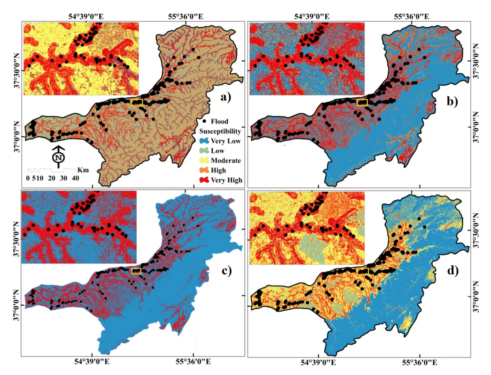
Our flood hazard susceptibility models have been developed using ML ensemble methods. These are capable of forecasting the susceptibility of flooding with the aid of various categorical factors. Flood hazard susceptibility maps (FSMs), based on Jenks’ natural break mechanisms, were divided into five subclasses: very high, high, moderate, low, and very low. The method of Jenks optimization, also called natural break classification, is a process of data segmentation to estimate the optimal value structure of the different classes. This method of classification aims to reduce the average disparity between classes while increasing the disparity from the rest of the class. The method thus eliminates intraclass and maximizes group disparities. A higher index rating represents areas that are particularly vulnerable to flooding, and vice versa. According to the J48 model, 46.63% of the basin area comes under the low flood susceptibility zone, whereas 18.67% and 29.13% of the area are very high and high flood-prone areas, respectively. The FSM generated using MJ48 suggested that 62.81% of the area falls into the very low flood susceptibility zone, whereas 24.6% of the basin is very highly prone to flooding (Table 3). The results generated in the RJ48 FSM suggested that 76.38% of the study basin has a very low flood occurrence probability, whereas 16.23% has a very high chance of flooding. The other categories have a significantly lower percentage of shares in terms of flood probability. Lastly, the RSJ48 ensemble method gives a less skewed result, predicting that 48.72% of the study area is a very low and 9.21% is a very high flood susceptibility zone, respectively (Figure 6). According to this model, 20.98% (Table 3) of the basin area is a moderately flood-prone region, which is the highest of all the models tested.
As per the output of the models, it is clear that the western and northwestern part of the study basin is a highly flood-susceptible region along with a few flanks of the southeastern and northeastern parts. The lowest elevations, slope, CI, SPI, and NDVI are located in these western and south-western parts of the study basin, which is the reason for the high to very high flood susceptibility along these zones. The rivers route water from the uphill areas and converge in this lower elevation region, which creates floods during the high rainfall periods. The natural setting of the region does not allow rapid transmission of flood water, resulting in numerous flood events. Accordingly, combination of geographic, geologic, and meteorological conditions are the main reasons for a higher propensity for flooding along this western part of the study basin.

3.4. Validation of Machine Learning Ensemble Models

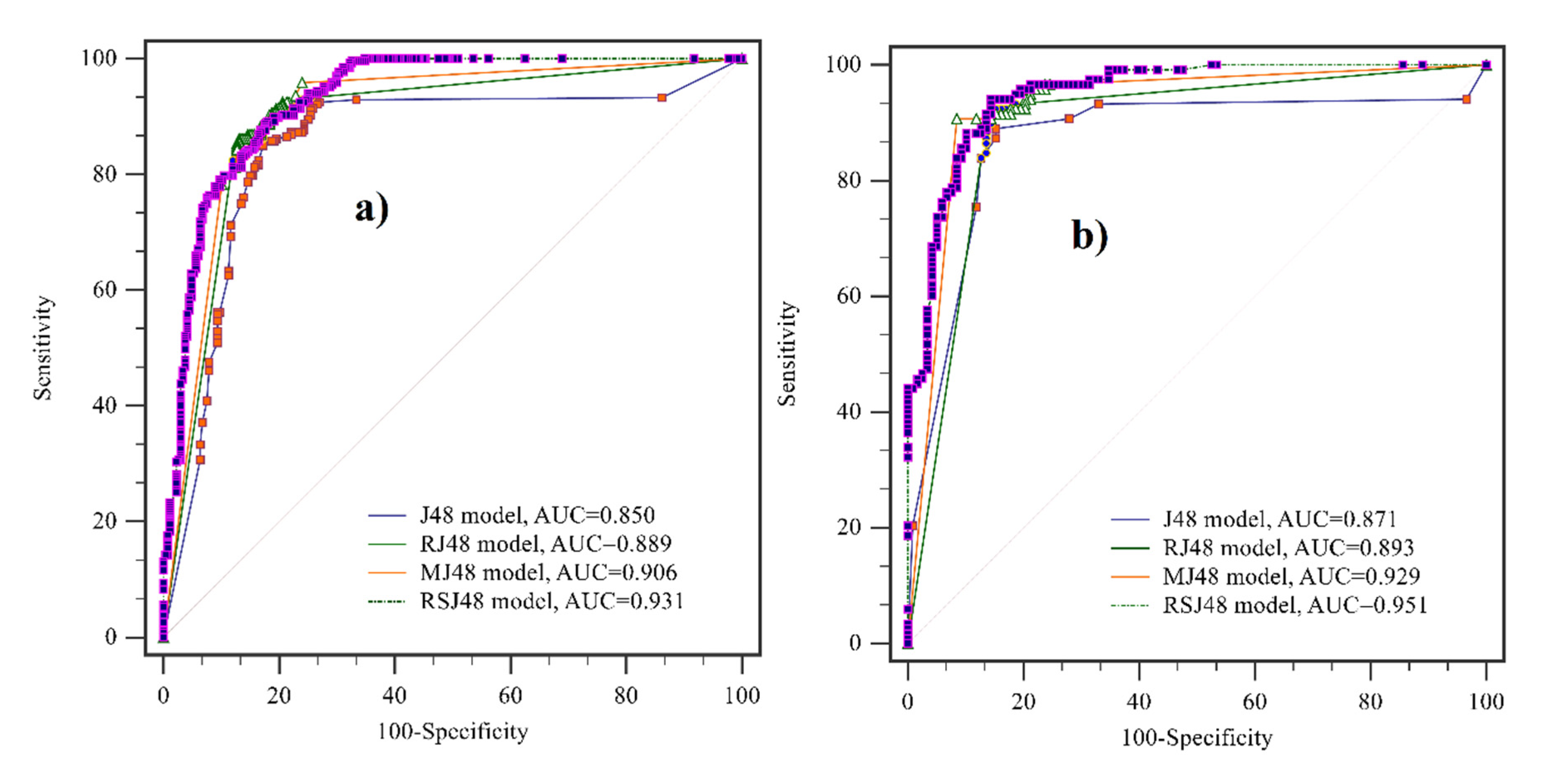
Often a single validation approach is inadequate because of the usage of limited samples to validate model results. In this analysis, the ML models performance was tested using the ROC curve, efficiency, and TSS methods. For the success rate curves of the training sample (70%), the RSJ48 model was more well fitted relative to the others, as the AUC value was the maximum (0.931) followed by MJ48 (0.901), RJ48 (0.889), and J48 (0.850), respectively (Figure 7a). The highest efficiency value was achieved by the RSJ48 model followed by MJ48, RJ48, and J48, respectively (Table 4). Similarly, for the training data the TSS and sensitivity values are highest for the RSJ48. The RMSE values of J48, MJ48, RJ48, and RSJ48 were 0.33, 0.35, 0.39, and 0.30, respectively.
A robust conclusion regarding the accuracy of predictions cannot be reached based on only training datasets. Prediction rate curves denote the predictive capacity of the models for future flood hazard susceptible zones in the study basin. The findings of the prediction rate curve suggest that the RSJ48 model is the most effective as the AUC was maximum (0.951) followed up by MJ48 (0.929). The efficiency values were 0.84, 0.84, 0.85, and 0.86, respectively of the J48, MJ48, RJ48, and RSJ48 models for the validation datasets, whereas TSS values for the J48, MJ48, RJ48, and RSJ48 models were 0.68, 0.70, 0.71, and 0.71, respectively. The sensitivity values for J48, MJ48, RJ48, and RSJ48 were 0.83, 0.80, 0.83, and 0.84, respectively (Table 4). The corresponding respective RMSE values were 0.35, 0.40, 0.34, and 0.33, respectively (Table 4).
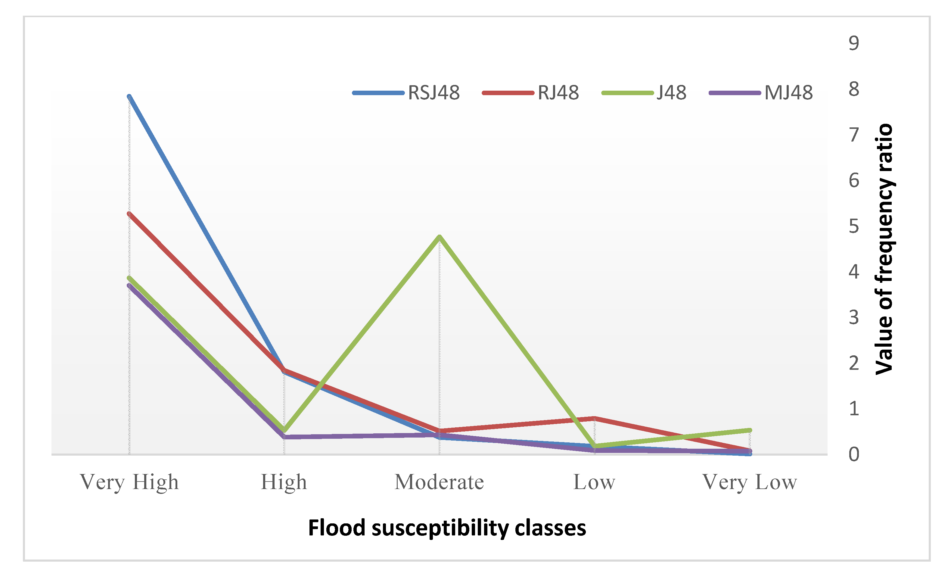
Figure 8 shows the values of FR for the selected models. Sub-class FR values were measured by dividing the amount of flood locations contained in the FS class and the total pixels of a particular FS class and the total number of flood location pixels by the FSM’s total pixel. Here, a higher value of FR for the very high FS class indicates the accuracy of the models and vice-versa. In our study, RSJ48 returned the highest FR value for the very high FS class and the lowest value for the very low FS class. However, other models also returned high FR values for the very high FS class.
On the basis of the above, it may be said that the ML ensemble models show uniform results for both success rate curves and prediction rate curves and that these are reasonably accurate. Therefore, these models can demarcate the flood hazard susceptibility zones in the study basin with higher precision compared to other models used by previous research. The RSJ48 model is better able to accurately map the FS within the study area, according to the AUC of the ROC curve, the efficiency and TSS methods, than the other ensemble methods we evaluated.

3.5. Sensitivity Analysis

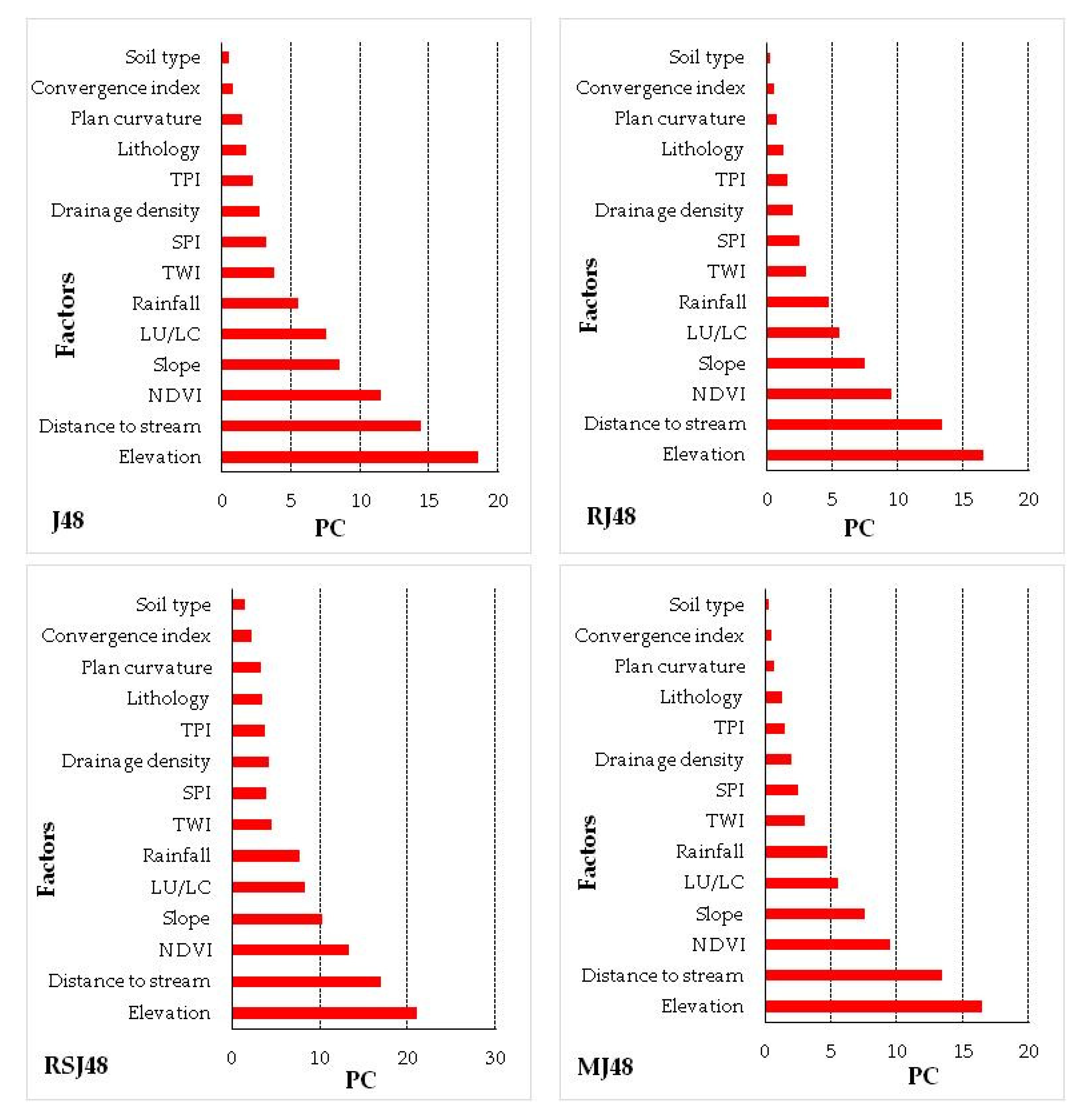
A sensitivity research was conducted to determine the FCF’s impact on the estimation of flood susceptibility. The results were summarized as percentage contribution (PC; Table 5 and Figure 9). Flood susceptibility maps produced by the ensemble ML method had the greatest sensitivity to elevation, followed by distance to the stream, NDVI, slope, LU/LC, rainfall, TWI, SPI, drainage density TPI, lithology, convergence index and soil type (Figure 9). Study of sensitivity may help in understanding the significant geo-environmental factor, which are very relevant for understanding the model structure in question. According to the sensitivity evaluation, in the case of RSJ48, every factor had a greater percentage contribution compared to the other ML models. Therefore, based on the analysis, it can be said that RSJ48 is better than the other models we tested.

4. Discussion

4.1. Model Performance and Comparison

Identification and zonation of flood-prone areas in a watershed are essential for reducing the damage caused by flooding. Until now, several methodologies have been developed by the researchers around the world for FSM [35,108,125], and each of them has drawbacks and advantages. Remote Sensing (RS) and Geographic Information System (GIS) are quite powerful and effective in analyzing multidimensional incidents like flooding that are affected by many controlling factors [35,126,127]. The widely used conventional machine learning models like artificial neural network (ANN), SVM, and Random Forest (RF) are well capable of predicting flood but ensemble of machine learning algorithms with any statistical or other machine learning techniques provide better result than the single method [32,33,37]. The decision tree based methods like ANN, SVM, and RF gives flexibility in nonlinear applications with large database and these are very much effective in flood modeling but whenever any ensemble classifiers are applied with them, the problem of over-fitting as well as prediction error gets reduced significantly. In this study, we developed flood susceptibility models using ML methods (hybrid J48 approaches) with one of three ensemble techniques (Real AdaBoost, Random Subspace, and MultiBoost). Ensemble approaches combine the art of data mining for classification while the J48 is a tree classifier considered to have good performance in forecasting flood susceptibility. Hybrid ML ensemble frameworks have been shown to deliver preferential outcomes for spatial flood estimation [128,129]. The imperative to implement such models and to develop an appropriate framework for risk management of flood hazards derives from the fact that floods are responsible for significant economic loss and destruction of human infrastructure and natural environments [30,31]. The findings of our study revealed that the accuracy of the J48 model (SRC = 0.850, PRC = 0.871, TSS = 72, E = 0.86) was enhanced after the ensemble with all three meta-classifiers. Our findings are rational as the ensemble classifiers reduce overfitting problems in FS modeling to improve the efficiency of base classifiers [128,130]. The used ensemble models in the study were shown better accuracy than the single model used in the flood studies (8, 10, 24, 31). The results of our analysis show that the RSJ48 model (AUC = 0.931, E = 0.89, TSS = 0.78, sensitivity = 0.87, and RMSE = 0.3 for testing dataset and AUC = 0.951, E = 0.86, TSS = 0.71, sensitivity = 0.84, and RMSE = 0.33 for training dataset) has the maximum predictive power, followed by the MJ48 model and the RJ48 model. The explanation for that the Random Subspace ensemble is more effective in minimizing uncertainty and discrimination compared to other ensemble approaches [131,132] and takes samples at different spatial layers from randomly chosen subspaces [58,101]. All of the models used in this research are efficient enough for predicting the flood susceptibility. The main advantage of these methods is that these can handle both the data mean continuous and categorical simultaneously. CRAN RWeka, party, regRSM packages of R studio were used for preparing these models. The RMSE of these models are low and, particularly for RSJ48, is very low. Besides, in terms of execution time and computational resources consumption, the RSJ48 model performs better than the other models used here.

4.2. Factor Contribution Analysis

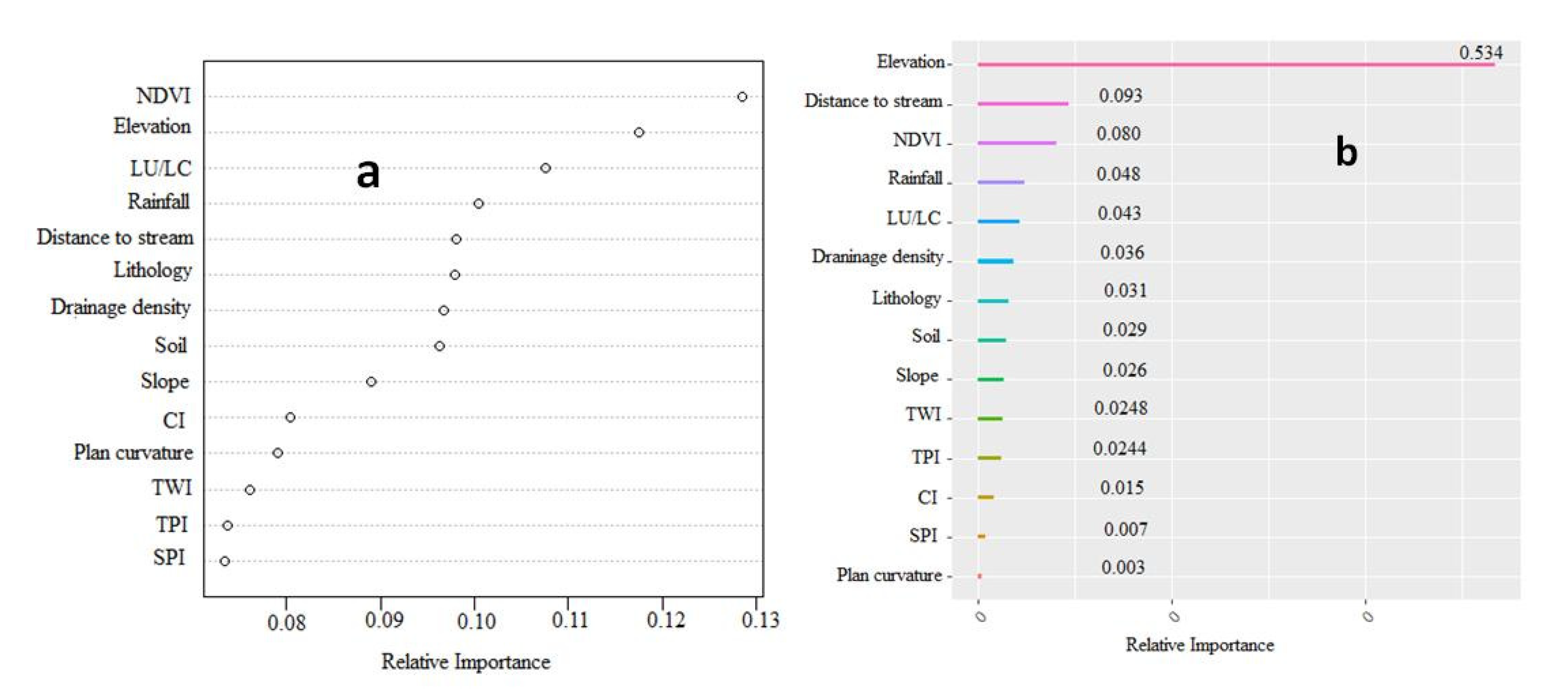
Flood hazard susceptibility delineation depends on the interplay of the FCFs. In this analysis, the Real AdaBoost and boosted regression tree (BRT) were used to calculate the relative merits of the chosen variables. The non-parametric model of ML approaches is BRT, which defines a relationship between dependent and independent variables [133]. This is a key tool for evaluating the relevancy of a particular variable and addressing classification and forecasting problems [134]. Details regarding the BRT are available in the literatures of Breiman et al. [134], Therneau et al. [135] and Friedman et al. [101]. We tested fourteen factors and, based on the results, we can identify the relative importance of the factors for flood susceptibility. According to the Real AdaBoost model, NDVI, elevation, LU/LC, rainfall, and stream distance are the top five most significant flood conditioning factors in descending order, whereas SPI, TPI, and TWI are the least relevant variables (Figure 10). However, using the BRT, elevation was determined to be the most important factor controlling flood hazard susceptibility with the highest importance value of 0.534, preceded by distance to stream (0.093), NDVI (0.080), rainfall (0.048), and LU/LC (0.043). Here, plan curvature (0.003) and SPI (0.007) were the two least important factors for flooding susceptibility.

5. Conclusions

Flooding hazards are very sensitive and devastating issues in the world. Recurring flood events cause a huge loss of human life and damage to properties, which should be mitigated at every possible level. Flash floods are a real threat to the sustainability of our societies. Therefore, the accurate prediction of susceptibility to flood events is necessary to improve management practices in effort to reduce flood damage. This work investigated the application of ML ensemble models for predicting flood hazard susceptibility zones in the study basin, along with the identification of the key controlling variables. The ML models suggested that 9.21% to 18.67% of the study basin has a very high susceptibility to flooding. The meta-classifiers we tested increased the accuracy of the J48 machine learning model. Of the three new ensemble models we tested, RSJ48 has better accuracy. Remote sensing and geographical information system integrating with the ML algorithms are creating great foundations for the management of different natural hazards. However, the present work will provide some guidance to other researchers wanting to apply ML ensemble methods to investigate susceptibility to flooding. More applications of the methods reported herein are, however, needed to assess the full extent of the suitability of our methods beyond the case study.

Supplementary Materials

The following are available online at https://www.mdpi.com/2072-4292/12/20/3423/s1.

Author Contributions

Conceptualization, A.A.; methodology, A.A.; formal analysis, A.A.; W.C.; investigation, A.A.; resources, A.A.; supervision, A.A.; writing—original draft preparation, A.A. S.S., K.M., writing—review and editing, A.A. S.S., K.M., T.B., P.T.T.N., S.S.B.; visualization, A.A.; supervision, A.A., S.S.B.; funding acquisition, T.B. All authors have read and agreed to the published version of the manuscript.

Funding

Open Access was funded by the Austrian Science Fund (FWF) through the Doctoral College GIScience (DK W 1237-N23) at the University of Salzburg.

Acknowledgments

Open Access Funding by the Austrian Science Fund (FWF).

Conflicts of Interest

The authors declare no conflict of interest.

References

  1. Asgharpour, S.E.; Ajdari, B.A. Case Study on Seasonal Floods in Iran, Watershed of Ghotour Chai Basin. Procedia Soc. Behav. Sci. 2011, 19, 556–566. [Google Scholar] [CrossRef] [Green Version]
  2. Keesstra, S.D. Impact of natural reforestation on floodplain sedimentation in the Dragonja basin, SW Slovenia. Earth Surf. Process. Landf. J. Br. Geomorphol. Res. Group 2007, 32, 49–65. [Google Scholar] [CrossRef]
  3. Vinet, F. Geographical analysis of damage due to flash floods in southern France: The cases of 12–13 November 1999 and 8–9 September 2002. Appl. Geogr. 2008, 28, 323–336. [Google Scholar] [CrossRef]
  4. Gharaibeh, A.A.; Zu’bi, A.; Esra’a, M.; Abuhassan, L.B. Amman (City of Waters); Policy, Land Use, and Character Changes. Land 2019, 8, 195. [Google Scholar] [CrossRef] [Green Version]
  5. Adnan, M.S.G.; Dewan, A.; Zannat, K.E.; Abdullah, A.Y.M. The use of watershed geomorphic data in flash flood susceptibility zoning: A case study of the Karnaphuli and Sangu river basins of Bangladesh. Nat. Hazards 2019, 99, 425–448. [Google Scholar] [CrossRef]
  6. Hirabayashi, Y.; Mahendran, R.; Koirala, S.; Konoshima, L.; Yamazaki, D.; Watanabe, S.; Kim, H.; Kanae, S. Global flood risk under climate change. Nat. Clim. Chang. 2013, 3, 816. [Google Scholar] [CrossRef]
  7. CRED; UNISDR. The Human Cost of Weather-Related Disasters, 1995–2015; United Nations: Geneva, Switzerland, 2015.
  8. Casale, R.; Margottini, C. Floods and Landslides, Integrated Risk Assessment, Integrated Risk Assessment; with 30 Tables; Springer Science & Business Media: Berlin, Germany, 1999. [Google Scholar]
  9. Smith, K. Environmental Hazards, Assessing Risk and Reducing Disaster; Routledge: Abingdon, UK, 2013. [Google Scholar]
  10. Paul, G.C.; Saha, S.; Hembram, T.K. Application of the GIS-Based Probabilistic Models for Mapping the Flood Susceptibility in Bansloi Sub-basin of Ganga-Bhagirathi River and Their Comparison. Remote Sens. Earth Syst. Sci. 2019, 15, 120–146. [Google Scholar] [CrossRef]
  11. Adnan, M.S.G.; Talchabhadel, R.; Nakagawa, H.; Hall, J.W. The potential of Tidal River Management for flood alleviation in South Western Bangladesh. Sci. Total Environ. 2020, 731, 138747. [Google Scholar] [CrossRef]
  12. Keesstra, S.D.; Bouma, J.; Wallinga, J.; Tittonell, P.; Smith, P.; Bardgett, R.D. The significance of soils and soil science towards realization of the United Nations Sustainable Development Goals. Soil 2016, 2, 111–128. [Google Scholar] [CrossRef] [Green Version]
  13. Keesstra, S.; Mol, G.; de Leeuw, J.; Okx, J.; de Cleen, M.; Visser, S. Soil-related sustainable development goals: Four concepts to make land degradation neutrality and restoration work. Land 2018, 7, 133. [Google Scholar] [CrossRef] [Green Version]
  14. Visser, S.; Keesstra, S.; Maas, G.; De Cleen, M. Soil as a Basis to Create Enabling Conditions for Transitions Towards Sustainable Land Management as a Key to Achieve the SDGs by 2030. Sustainability 2019, 11, 6792. [Google Scholar] [CrossRef] [Green Version]
  15. Algeria: State Owned Reinsurer Shows Strong Technical Results, Good Investment Returns. Available online: https://www.meinsurancereview.com/News/View-NewsLetterArticle?id=46352&Type=MiddleEast (accessed on 20 September 2019).
  16. Norouzi, G.; Taslimi, M. The impact of flood damages on production of Iran’s agricultural sector. Middle East J. Sci. Res. 2012, 12, 921–926. [Google Scholar]
  17. Jannati, H. History of the Devastating Floods in Iran. Political Studies and Research Institute 593 of Iran, pr 12. 2019. Available online: http//ir-psri.com/?Page=ViewNews&NewsID=6283 (accessed on 20 September 2019).
  18. Safaripour, M.; Monavari, M.; Zare, M.; Abedi, Z.; Gharagozlou, A. Flood Risk Assessment Using GIS (Case Study, Golestan Province, Iran). Pol. J. Environ. Stud. 2012, 21, 1817–1824. [Google Scholar]
  19. Mosavi, A.; Ozturk, P.; Chau, K.W. Flood Prediction Using Machine Learning Models: Literature Review. Water 2018, 10, 1536. [Google Scholar] [CrossRef] [Green Version]
  20. Kauffeldt, A.; Wetterhall, F.; Pappenberger, F.; Salamon, P.; Thielen, J. Technical review of large-scale hydrological models for implementation in operational flood forecasting schemes on continental level. Environ. Model. Softw. 2016, 75, 68–76. [Google Scholar] [CrossRef]
  21. Devia, G.K.; Ganasri, B.P.; Dwarakish, G.S. A Review on Hydrological Models. Aquat. Procedia 2015, 4, 1001–1007. [Google Scholar] [CrossRef]
  22. Chourushi, S.; Lodha, P.; Prakash, I. A Critical Review of Hydrological Modeling Practices for Flood Management. Pramana Res. J. 2019, 9, 352–362. [Google Scholar]
  23. Sanz-Ramos, M.; Amengual, A.; Bladé Castellet, E.; Romero, R.; Roux, H. Flood forecasting using a coupled hydrological and hydraulic model (based on FVM) and highresolution meteorological model. E3S Web Conf. 2018, 40, 06028. [Google Scholar] [CrossRef]
  24. Unduche, F.; Tolossa, H.; Senbeta, D.; Zhu, E. Evaluation of four hydrological models for operational flood forecasting in a Canadian Prairie watershed. Hydrol. Sci. J. 2018, 63, 1133–1149. [Google Scholar] [CrossRef] [Green Version]
  25. Costabile, P.; Macchione, F. Enhancing river model set-up for 2-D dynamic flood modelling. Environ. Model. Softw. 2015, 67, 89–107. [Google Scholar] [CrossRef]
  26. Fawcett, R.; Stone, R.A. Comparison of two seasonal rainfall forecasting systems for Australia. Aust. Meteorol. Oceanogr. J. 2010, 60, 15–24. [Google Scholar] [CrossRef]
  27. Arabameri, A.; Karimi-Sangchini, E.; Chandra Pal, S.; Saha, A.; Chowdhuri, I.; Lee, S.; Tien Bui, D. Novel Credal Decision Tree-Based Ensemble Approaches for Predicting the Landslide Susceptibility. Remote Sens. 2020, 12, 3389. [Google Scholar] [CrossRef]
  28. Ji, J.; Choi, C.; Yu, M.; Yi, J. Comparison of a data-driven model and a physical model for flood forecasting. WIT Trans. Ecol. Environ. 2012, 159, 133–142. [Google Scholar] [CrossRef] [Green Version]
  29. Nampak, H.; Pradhan, B.; Manap, M.A. Application of GIS based data driven evidential belief function model to predict groundwater potential zonation. J. Hydrol. 2014, 513, 283–300. [Google Scholar] [CrossRef]
  30. Tehrany, M.S.; Pradhan, B.; Jebur, M.N. Spatial prediction of flood susceptible areas using rule based decision tree (DT) and a novel ensemble bivariate and multivariate statistical models in GIS. J. Hydrol. 2013, 11, 69–79. [Google Scholar] [CrossRef]
  31. Youssef, A.M.; Pradhan, B.; Sefry, S.A. Flash flood susceptibility assessment in Jeddah city (Kingdom of Saudi Arabia) using bivariate and multivariate statistical models. Environ. Earth Sci. 2016, 75, 12. [Google Scholar] [CrossRef]
  32. Hong, H.; Liu, J.; Bui, D.T.; Pradhan, B.; Acharya, T.D.; Pham, B.T. Landslide susceptibility mapping using J48 decision tree with AdaBoost, bagging and rotation forest ensembles in the Guangchang area (China). Catena 2018, 163, 399–413. [Google Scholar] [CrossRef]
  33. Hong, H.; Tsangaratos, P.; Ilia, I.; Liu, J.; Zhu, A.X.; Chen, W. Application of fuzzy weight of evidence and datamining techniques in construction of flood susceptibility map of Poyang County, China. Sci. Total Environ. 2018, 625, 575–588. [Google Scholar] [CrossRef]
  34. Tien Bui, D.; Pradhan, B.; Nampak, H.; Bui, Q.T.; Tran, Q.A.; Nguyen, Q.P. Hybrid artificial intelligence approach based on neural fuzzy inference model and meta heuristic optimization for flood susceptibility modeling in a high-frequency tropical cyclone area using GIS. J. Hydrol. 2016, 540, 317–330. [Google Scholar] [CrossRef]
  35. Tehrany, M.S.; Pradhan, B.; Jebur, M.N. Flood susceptibility analysis and its verification using a novel ensemble support vector machine and frequency ratio method. Stoch. Environ. Res. Risk Assess. 2015, 29, 1149–1165. [Google Scholar] [CrossRef]
  36. Tehrany, M.S.; Kumar, L. The application of a Dempster–Shafer-based evidential belief function in flood susceptibility mapping and comparison with frequency ratio and logistic regression methods. Environ. Earth Sci. 2018, 77, 490. [Google Scholar] [CrossRef]
  37. Arabameri, A.; Rezaei, K.; Cerdà, A.; Conoscenti, C.; Kalantari, Z. A comparison of statistical methods and multi-criteria decision making to map flood hazard susceptibility in Northern Iran. Sci. Total Environ. 2019, 660, 443–458. [Google Scholar] [CrossRef] [PubMed]
  38. Radmehr, A.; Araghinejad, S. Developing strategies for urban flood management of Tehran city using SMCDM and ANN. J. Comput. Civ. Eng. 2014, 28, 05014006. [Google Scholar] [CrossRef]
  39. Chen, Y.R.; Yeh, C.H.; Yu, B. Integrated application of the analytic hierarchy process and the geographic information system for flood risk assessment and flood plain management in Taiwan. Nat. Hazards 2011, 59, 1261–1276. [Google Scholar] [CrossRef] [Green Version]
  40. Stefanidis, S.; Stathis, D. Assessment of flood hazard based on natural and anthropogenic factors using analytic hierarchy process (AHP). Nat. Hazards 2013, 68, 569–585. [Google Scholar] [CrossRef]
  41. Zou, Q.; Zhou, J.; Zhou, C.; Song, L.; Guo, J. Comprehensive flood risk assessment based on set pair analysis-variable fuzzy sets model and fuzzy AHP. Stoch. Environ. Res. Risk Assess. 2013, 27, 525–546. [Google Scholar] [CrossRef]
  42. Kazakis, N.; Kougias, I.; Patsialis, T. Assessment of flood hazard areas at a regional scale using an index-based approach and Analytical Hierarchy Process, Application in Rhodope–Evros region, Greece. Sci. Total Environ. 2015, 538, 555–563. [Google Scholar] [CrossRef]
  43. Rahmati, O.; Pourghasemi, H.R.; Zeinivand, H. Flood susceptibility mapping using frequency ratio and weights-of-evidence models in the Golastan Province, Iran. Geocarto Int. 2016, 31, 42–70. [Google Scholar] [CrossRef]
  44. Lee, S.; Kim, Y.S.; Oh, H.J. Application of a weights-of-evidence method and GIS to regional groundwater productivity potential mapping. J. Environ. Manag. 2012, 96, 91–105. [Google Scholar] [CrossRef]
  45. Rahmati, O.; Nazari Samani, A.; Mahmoodi, N.; Mahdavi, M. Assessment of the contribution of N-fertilizers to nitrate pollution of groundwater in western Iran (case study, Ghorveh–DehgelanArquifer). Water Qual. Expo. Health 2015, 7, 143–151. [Google Scholar] [CrossRef]
  46. Arabameri, A.; Chen, W.; Blaschke, T.; Tiefenbacher, J.P.; Pradhan, B.; Bui, D.T. Gully Head-Cut Distribution Modeling Using Machine Learning Methods—A Case Study of N.W. Iran. Water 2020, 12, 16. [Google Scholar] [CrossRef] [Green Version]
  47. Arabameri, A.; Cerda, A.; Pradhan, B.; Tiefenbacher, J.P.; Lombardo, L.; Bui, D.T. A methodological comparison of head-cut based gully erosion susceptibility models: Combined use of statistical and artificial intelligence. Geomorphology 2020, 107136. [Google Scholar] [CrossRef]
  48. Arabameri, A.; Lee, S.; Tiefenbacher, J.P.; Ngo, P.T.T. Novel Ensemble of MCDM-Artificial Intelligence Techniques for Groundwater-Potential Mapping in Arid and Semi-Arid Regions (Iran). Remote Sens. 2020, 12, 490. [Google Scholar] [CrossRef] [Green Version]
  49. Arabameri, A.; Blaschke, T.; Pradhan, B.; Pourghasemi, H.R.; Tiefenbacher, J.P.; Bui, D.T. Evaluation of Recent Advanced Soft Computing Techniques for Gully Erosion Susceptibility Mapping: A Comparative Study. Sensors 2020, 20, 335. [Google Scholar] [CrossRef] [Green Version]
  50. Pham, B.T.; Tien Bui, D.; Prakash, I.; Dholakia, M.B. Rotation forest fuzzy rule-based classifier ensemble for spatial prediction of landslides using GIS. Nat. Hazards 2016, 83, 97–127. [Google Scholar] [CrossRef]
  51. Althuwaynee, O.F.; Pradhan, B.; Lee, S. Application of an evidential belief function model in landslide susceptibility mapping. Comput. Geosci. 2012, 44, 120–135. [Google Scholar] [CrossRef]
  52. Chen, W.; Shirzadi, A.; Shahabi, H.; Ahmad, B.B.; Zhang, S.; Hong, H. A novel hybrid artificial intelligence approach based on the rotation forest ensemble and naive Bayes tree classifiers for a landslide susceptibility assessment in Langao County, China. Geomat. Nat. Hazards Risk 2017, 8, 1955–1977. [Google Scholar] [CrossRef] [Green Version]
  53. Tien Bui, D.; Tuan, T.A.; Hoang, N.-D.; Thanh, N.Q.; Nguyen, D.B.; Van Liem, N. Spatial prediction of rainfall-induced landslides for the Lao Cai area (Vietnam) using a hybrid intelligent approach of least squares support vector machines inference model and artificial bee colony optimization. Landslides 2017, 14, 447–458. [Google Scholar] [CrossRef]
  54. Kordestani, M.D.; Naghibi, S.A.; Hashemi, H.; Ahmadi, K.; Kalantar, B.; Pradhan, B. Groundwater potential mapping using a novel data-mining ensemble model. J. Hydrol. 2019, 27, 211–224. [Google Scholar] [CrossRef] [Green Version]
  55. Rahmati, O.; Naghibi, S.A.; Shahabi, H.; Bui, D.T.; Pradhan, B.; Azareh, A.; Melesse, A.M. Groundwater spring potential modelling, Comprising the capability and robustness of three different modeling approaches. J. Hydrol. 2018, 565, 248–261. [Google Scholar] [CrossRef]
  56. Hosseini, F.S.; Choubin, B.; Mosavi, A. Flash-flood hazard assessment using ensembles and Bayesian-based machine learning models: Application of the simulated annealing feature selection method. Sci. Total Environ. 2020, 711, 135161. [Google Scholar] [CrossRef]
  57. Janizadeh, S.; Avand, M.; Jaafari, A. Prediction Success of Machine Learning Methods for Flash Flood Susceptibility Mapping in the Tafresh Watershed, Iran. Sustainability 2019, 11, 5426. [Google Scholar] [CrossRef] [Green Version]
  58. Edwards, P.K.; Duhon, D.; Shergill, S. Real AdaBoost, Boosting for Credit Scorecards and Similarity to WOE Logistic Regression; Scotiabank: Toronto, ON, Canada, 2019; pp. 1323–2017. [Google Scholar]
  59. Tao, D.; Tang, X.; Li, X.; Wu, X. Asymmetric bagging and random subspace for support vector machines-based relevance feedback in image retrieval. IEEE Trans. Pattern Anal. Mach. Intell. 2006, 28, 1088–1099. [Google Scholar] [PubMed] [Green Version]
  60. Nanni, L.; Lumini, A. Random subspace for an improved biohashing for face authentication. Pattern Recogn. Lett. 2008, 29, 295–300. [Google Scholar] [CrossRef]
  61. Zhang, X.; Jia, Y. A linear discriminant analysis framework based on random subspace for face recognition. Pattern Recognit. 2007, 40, 2585–2591. [Google Scholar] [CrossRef]
  62. Zhu, Y.; Liu, J.; Chen, S. Semi-random subspace method for face recognition. Image Vis. Comput. 2009, 27, 1358–1370. [Google Scholar] [CrossRef] [Green Version]
  63. Hong, H.; Liu, J.; Zhu, A.X.; Shahabi, H.; Pham, B.T.; Chen, W.; Pradhan, B.; Bui, D.T. A novel hybrid integration model using support vector machines and random subspace for weather-triggered landslide susceptibility assessment in the Wuning area (China). Environ. Earth Sci. 2017, 76, 652. [Google Scholar] [CrossRef]
  64. Webb, G.I. MultiBoosting, a technique for combining boosting and wagging. Mach. Learn. 2000, 40, 159–196. [Google Scholar] [CrossRef] [Green Version]
  65. IRIMO. Summary Reports of Iran’s Extreme Climatic Events. Ministry of Roads and Urban Development, Iran Meteorological Organization. 2012. Available online: www.cri.ac.ir (accessed on 20 September 2019).
  66. GSI. Geology Survey of Iran. 1997. Available online: http//www.gsi.ir/Main/Lang_en/index.html (accessed on 20 September 2019).
  67. Donya-e-Eqtesad. 2019. Available online: https//www.donya-e-eqtesad.com/fa/tiny/news-5863511460 (accessed on 20 September 2019).
  68. Hasan, M.K.; Kumar, L.; Gopalakrishnan, T. Inundation modelling for Bangladeshi coasts usingdownscaled and bias-corrected temperature. Clim. Risk Manag. 2020, 27, 100207. [Google Scholar] [CrossRef]
  69. Gesch, D.; Oimoen, M.; Zhang, Z.; Meyer, D.; Danielson, J. Validation of the ASTER global digital elevation model version 2 over the conterminous United States. Int. Arch. Photogramm. Remote Sens. Spat. Inf. Sci. 2012, B4, 281–286. [Google Scholar]
  70. Arabameri, A.; Saha, S.; Chen, W.; Roy, J.; Pradhan, B.; Bui, D.T. Flash flood susceptibility modelling using functional tree and hybrid ensemble techniques. J. Hydrol. 2020, 587, 125007. [Google Scholar] [CrossRef]
  71. Arabameri, A.; Pradhan, B.; Bui, D.T. Spatial modelling of gully erosion in the Ardib River Watershed using three statistical-based techniques. Catena 2020, 190, 104545. [Google Scholar] [CrossRef]
  72. Zakerinejad, R.; Maerker, M. Prediction of gully erosion susceptibilities using detailed terrain analysis and maximum entropy modeling: A case study in the Mazayejan Plain, Southwest Iran. Suppl. Geogr. Fis. Din. Quat. 2014, 37, 67–76. [Google Scholar]
  73. Bui, D.T.; Ho, T.C.; Pradhan, B.; Pham, B.T.; Nhu, V.H.; Revhaug, I. GIS-based modeling of rainfall-induced landslides using data mining-based functional trees classifier with AdaBoost, Bagging, and MultiBoost ensemble frameworks. Environ. Earth Sci. 2016, 75, 1101. [Google Scholar]
  74. Khosravi, K.; Pourghasemi, H.R.; Chapi, K.; Bahri, M. Flash flood susceptibility analysis and its mapping using different bivariate models in Iran: A comparison between Shannon’s entropy, statistical index, andweighting factor models. Environ. Monit. Assess. 2016, 188, 656. [Google Scholar] [CrossRef] [PubMed]
  75. Meraj, G.; Romshoo, S.A.; Yousuf, A.R.; Altaf, S.; Altaf, F. Assessing the influence of watershed characteristics on the flood vulnerability of Jhelum basin in Kashmir Himalaya. Nat. Hazards 2015, 77, 153–175. [Google Scholar] [CrossRef]
  76. Khosravi, K.; Nohani, E.; Maroufinia, E.; Pourghasemi, H.R. A GIS-based flood susceptibility assessment and its mapping in Iran, a comparison between frequency ratio and weights-of-evidence bivariate statistical models with multi-criteria decision-making technique. Nat. Hazards 2016, 83, 947–987. [Google Scholar] [CrossRef]
  77. Botzen, W.J.W.; Aerts, J.C.J.H.; van den Bergh, J.C.J.M. Individual preferences for reducing flood risk to near zero through elevation. Mitig. Adapt. Strateg. Glob. Chang. 2012, 2, 229–244. [Google Scholar] [CrossRef] [Green Version]
  78. Kirkby, M.J.; Beven, K.J. A physically based, variable contributing area model of basin hydrology. Hydrol. Sci. Bull. 1979, 24, 43–69. [Google Scholar]
  79. Gokceoglu, C.; Sonmez, H.; Nefeslioglu, H.A.; Duman, T.Y.; Can, T. The 17 March 2005 Kuzulu landslide (Sivas, Turkey) and landslide-susceptibility map of its near vicinity. Eng. Geol. 2005, 81, 65–83. [Google Scholar] [CrossRef]
  80. Riley, S.J.; De Gloria, S.D.; Elliot, R. A terrain ruggedness index that quantifies topographic heterogeneity. Intermt. J. Sci. 1999, 5, 23–27. [Google Scholar]
  81. Gallant, J.C.; Wilson, J.P. Primary topographic attributes. In Terrain Analysis, Principles and Applications; Wilson, J.P., Gallant, J.C., Eds.; Wiley: New York, NY, USA, 2000; pp. 51–85. [Google Scholar]
  82. Weiss, A. Topographic position and landforms analysis. In Proceedings of the Poster Presentation, ESRI User Conference, San Diego, CA, USA, 9 July 2001; Volume 200. [Google Scholar]
  83. Grohmann, C.H.; Riccomini, C. Comparison of roving-window and search-window techniques for characterising landscape morphometry. Comput. Geosci. 2009, 35, 2164–2169. [Google Scholar] [CrossRef] [Green Version]
  84. Moore, I.D.; Grayson, R.B.; Ladson, A.R. Digital terrain modelling: A review of hydrological, geomorphological, and biological applications. Hydrol. Process. 1991, 5, 3–30. [Google Scholar] [CrossRef]
  85. Kiss, R. Determination of drainage network in digital elevation model, utilities and limitations. J. Hung. Geo-Math. 2004, 2, 16–29. [Google Scholar]
  86. Khosravi, K.; Pham, B.T.; Chapi, K.; Shirzadi, A.; Shahabi, H.; Revhaug, I. A comparative assessment of decision trees algorithms for flash flood susceptibility modeling at Haraz watershed, northern Iran. Sci. Total Environ. 2018, 627, 744–755. [Google Scholar] [CrossRef]
  87. Opperman, J.J.; Galloway, G.E.; Fargione, J.; Mount, J.F.; Richter, B.D.; Secchi, S. Sustainable floodplains through large-scale reconnection to rivers. Science 2009, 3265959, 1487–1488. [Google Scholar] [CrossRef]
  88. Boer, E.P.; de Beurs, K.M.; Hartkamp, A.D. Kriging and thin plate splines for mapping climate variables. Int. J. Appl. Earth Obs. Geoinf. 2001, 3, 146–154. [Google Scholar] [CrossRef]
  89. Sajedi-Hosseini, F.; Choubin, B.; Solaimani, K.; Cerdà, A.; Kavian, A. Spatial prediction of soil erosion susceptibility using a fuzzy analytical network process, Application of the fuzzy decision-making trial and evaluation laboratory approach. Land Degrad. Dev. 2018, 29, 3092–3103. [Google Scholar] [CrossRef]
  90. Lo, C.P.; Yeung, A.K.W. Concepts and Techniques of Geographic Information System; Pearson Education Inc.: Hoboken, NJ, USA, 2002. [Google Scholar]
  91. Pradhan, B. Flood susceptible mapping and risk area estimation using logistic regression, GIS and remote sensing. J. Spat. Hydrol. 2010, 9, 1–18. [Google Scholar]
  92. Arabameri, A.; Nalivan, O.A.; Saha, S.; Roy, J.; Pradhan, B.; Tiefenbacher, J.P.; Ngo, P.T.T. Novel Ensemble Approaches of Machine Learning Techniques in Modeling the Gully Erosion Susceptibility. Remote Sens. 2020, 12, 1890. [Google Scholar] [CrossRef]
  93. Arabameri, A.; Chen, W.; Lombardo, L.; Blaschke, T.; Tien Bui, D. Hybrid Computational Intelligence Models for Improvement Gully Erosion Assessment. Remote Sens. 2020, 12, 140. [Google Scholar] [CrossRef] [Green Version]
  94. Arabameri, A.; Chen, W.; Loche, M.; Zhao, X.; Li, Y.; Lombardo, L.; Cerda, A.; Pradhan, B.; Bui, D.T. Comparison of machine learning models for gully erosion susceptibility mapping. Geosci. Front. 2020, 11, 1609–1620. [Google Scholar] [CrossRef]
  95. Roy, J.; Saha, S.; Arabameri, A.; Blaschke, T.; Bui, D.T. A Novel Ensemble Approach for Landslide Susceptibility Mapping (LSM) in Darjeeling and Kalimpong Districts, West Bengal, India. Remote Sens. 2019, 11, 2866. [Google Scholar] [CrossRef] [Green Version]
  96. Arabameri, A.; Cerda, A.; Rodrigo-Comino, J.; Pradhan, B.; Sohrabi, M.; Blaschke, T.; Bui, D.T. Proposing a Novel Predictive Technique for Gully Erosion Susceptibility Mapping in Arid and Semi-arid Regions (Iran). Remote Sens. 2019, 11, 2577. [Google Scholar] [CrossRef] [Green Version]
  97. Gayen, A.; Pourghasemi, H.R.; Saha, S.; Keesstra, S.; Bai, S. Gully erosion susceptibility assessment and management of hazard-prone areas in India using different machine learning algorithms. Sci. Total Environ. 2019, 668, 124–138. [Google Scholar] [CrossRef]
  98. Lee, S.; Pradhan, B. Landslide hazard mapping at Selangor, Malaysia using frequency ratio and logistic regression models. Landslides 2006, 4, 33–41. [Google Scholar] [CrossRef]
  99. Kaur, G.; Chhabra, A. Improved J48 classification algorithm for the prediction of diabetes. Int. J. Comput. Appl. 2014, 98, 13–17. [Google Scholar] [CrossRef]
  100. Witten, H.I.; Frank, E.; Mark, A. Hall Data Mining: Practical Machine Learning Tools and Techniques, 3rd ed.; Morgan Kaufmann: Burlington, MA, USA, 2011; p. 664. [Google Scholar]
  101. Freund, Y.; Schapire, R.E. A decision-theoretic generalization of on-line learning and an application to boosting. J. Comput. Syst. Sci. 1997, 55, 119–139. [Google Scholar] [CrossRef] [Green Version]
  102. Friedman, H.; Hastie, T.; Tibshirani, R. Additive logistic regression, a statistical view of boosting. Ann. Stat. 2000, 28, 337–407. Available online: https//web.stanford.edu/~hastie/Papers/AdditiveLogisticRegression/alr.pdf (accessed on 25 September 2019). [CrossRef]
  103. Ho, T.K. Nearest neighbors in random subspaces. In Joint IAPR International Workshops on Statistical Techniques in Pattern Recognition (SPR) and Structural and Syntactic Pattern Recognition (SSPR); Springer: Berlin/Heidelberg, Germany, 1998; pp. 640–648. [Google Scholar]
  104. Kotsiantis, S. Combining bagging, boosting, rotation forest and random subspace methods. Artif. Intell. Rev. 2011, 35, 223–240. [Google Scholar] [CrossRef]
  105. Kuncheva, L.I.; Rodrı’guez, J.J.; Plumpton, C.O.; Linden, D.E.; Johnston, S.J. Random subspace ensembles for fMRI classification. IEEE Trans. Med. Imaging 2010, 29, 531–542. [Google Scholar] [CrossRef]
  106. Mielniczuk, J.; Teisseyre, P. Using random subspace method for prediction and variable importance assessment in linear regression. Comput. Stat. Data Anal. 2014, 71, 725–742. [Google Scholar] [CrossRef]
  107. Sun, S.; Zhang, C. The selective random subspace predictor for traffic flow forecasting. IEEE Trans. Intell. Transp. Syst. 2007, 8, 367–373. [Google Scholar] [CrossRef]
  108. Chen, W.; Zhao, X.; Tsangaratos, P.; Shahabi, H.; Ilia, I.; Xue, W.; Wang, X.; Ahmad, B.B. Evaluating the usage of tree-based ensemble methods in groundwater spring potential mapping. J. Hydrol. 2020, 583, 124602. [Google Scholar] [CrossRef]
  109. Li, Y.; Chen, W. Landslide susceptibility evaluation using hybrid integration of evidential belief function and machine learning techniques. Water 2020, 12, 113. [Google Scholar] [CrossRef] [Green Version]
  110. Wang, G.; Lei, X.; Chen, W.; Shahabi, H.; Shirzadi, A. Hybrid computational intelligence methods for landslide susceptibility mapping. Symmetry 2020, 12, 325. [Google Scholar] [CrossRef] [Green Version]
  111. Lei, X.; Chen, W.; Pham, B.T. Performance evaluation of gis-based artificial intelligence approaches for landslide susceptibility modeling and spatial patterns analysis. ISPRS Int. J. Geo-Inform. 2020, 9, 443. [Google Scholar] [CrossRef]
  112. Chen, X.; Chen, W. Gis-based landslide susceptibility assessment using optimized hybrid machine learning methods. CATENA 2021, 196, 104833. [Google Scholar] [CrossRef]
  113. Zhao, X.; Chen, W. Gis-based evaluation of landslide susceptibility models using certainty factors and functional trees-based ensemble techniques. Appl. Sci. 2020, 10, 16. [Google Scholar] [CrossRef] [Green Version]
  114. Chen, W.; Li, Y. Gis-based evaluation of landslide susceptibility using hybrid computational intelligence models. CATENA 2020, 195, 104777. [Google Scholar] [CrossRef]
  115. Chen, W.; Chen, X.; Peng, J.; Panahi, M.; Lee, S. Landslide susceptibility modeling based on anfis with teaching-learning-based optimization and satin bowerbird optimizer. Geosci. Front. 2021, 12, 93–107. [Google Scholar] [CrossRef]
  116. Fukuda, S.; De Baets, B.; Waegeman, W.; Verwaeren, J.; Mouton, A.M. Habitat prediction and knowledge extraction for spawning European grayling (Thymallusthymallus L.) using a broad range of species distribution models. Environ. Modell. Softw. 2013, 47, 1–6. [Google Scholar] [CrossRef]
  117. Saltelli, A.; Chan, K.; Scott, E.M. Sensitivity Analysis; Wiley: New York, NY, USA, 2000. [Google Scholar]
  118. Crosetto, M.; Tarantola, S. Uncertainty and sensitivity analysis: Tools for GISbased model implementation. Int. J. Geogr. Inf. Sci. 2001, 15, 415–437. [Google Scholar] [CrossRef]
  119. Ferretti, F.; Saltelli, A.; Tarantola, S. Trends in sensitivity analysis practice in the last decade. Sci. Total Environ. 2016, 568, 666–670. [Google Scholar] [CrossRef] [PubMed]
  120. Chen, Y.; Yu, J.; Khan, S. Spatial sensitivity analysis of multi-criteria weights in GISbased land suitability evaluation. Environ. Model. Softw. 2010, 25, 1582–1591. [Google Scholar] [CrossRef]
  121. Lodwick, W.A.; Monson, W.; Svoboda, L. Attribute error and sensitivity analysis of map operations in geographical information systems: Suitability analysis. Int. J. Geogr. Inf. Syst. 1990, 4, 413–428. [Google Scholar] [CrossRef]
  122. Oh, H.J.; Kim, Y.S.; Choi, J.K.; Park, E.; Lee, S. GIS mapping of regional probabilistic groundwater potential in the area of Pohang City, Korea. J. Hydrol. 2011, 399, 158–172. [Google Scholar] [CrossRef]
  123. Fenta, A.A.; Kifle, A.; Gebreyohannes, T.; Hailu, G. Spatial analysis of groundwater potential using remote sensing and GIS-based multi-criteria evaluation in Raya Valley, northern Ethiopia. Hydrogeol. J. 2015, 23, 195–206. [Google Scholar] [CrossRef]
  124. Convertino, M.; Muñoz-Carpena, R.; Chu-Agor, M.L.; Kiker, G.L.; Linkov, I. Untangling drivers of species distributions: Global sensitivity and uncertainty analyses of MAXENT. Environ. Model. Softw. 2014, 51, 296–309. [Google Scholar] [CrossRef]
  125. Park, N.W. Using maximum entropy modeling for landslide susceptibility mapping with multiple geoenvironmental data sets. Environ. Earth Sci. 2015, 73, 937–949. [Google Scholar] [CrossRef]
  126. Arabameri, A.; Saha, S.; Roy, J.; Chen, W.; Blaschke, T.; Tien Bui, D. Landslide Susceptibility Evaluation and Management Using Different Machine Learning Methods in The Gallicash River Watershed, Iran. Remote Sens. 2020, 12, 475. [Google Scholar] [CrossRef] [Green Version]
  127. Arabameri, A.; Pradhan, B.; Lombardo, L. Comparative assessment using boosted regression trees, binary logistic regression, frequency ratio and numerical risk factor for gully erosion susceptibility modelling. Catena 2019, 183, 104223. [Google Scholar] [CrossRef]
  128. Pham, B.T.; Bui, D.T.; Prakash, I.; Dholakia, M.B. Hybrid integration of Multilayer Perceptron Neural Networks and machine learning ensembles for landslide susceptibility assessment at Himalayan area (India) using GIS. Catena 2017, 149, 52–63. [Google Scholar] [CrossRef]
  129. Tien Bui, D.; Tien Ho, C.; Revhaug, I.; Pradhan, B.; Duy Nguyen, B. Landslide susceptibility mapping along the national road 32 of Vietnam using GIS-based j48 decision tree classifier and its ensembles. In Cartography from Pole to Pole; Buchroithner, M., Prechtel, N., Burghardt, D., Eds.; Springer: Berlin/Heidelberg, Germany, 2014; pp. 303–317. [Google Scholar]
  130. Kuncheva, L.I. Combining Pattern Classifiers Methods and Algorithms; Wiley: Chichester, UK, 2004. [Google Scholar]
  131. Onan, A. On the performance of ensemble learning for automated diagnosis of breast cancer. Artif. Intell. Perspect. Appl. 2015, 347, 119–129. [Google Scholar]
  132. Robinzonov, N. Advances in Boosting of Temporal and Spatial Models. Ludwig-Maximilians-Universitat München. 2013. Available online: http://edoc.ub.uni-muenchen.de/15338/ (accessed on 20 September 2019).
  133. Aertsen, W.; Kint, V.; Van Orshoven, J. Evaluation of modelling techniques for forest site productivity prediction in contrasting ecoregions using stochastic multicriteria acceptability analysis (SMAA). Environ. Model. Softw. 2011, 26, 929–937. [Google Scholar] [CrossRef] [Green Version]
  134. Breiman, L. Arcing Classifiers. Ann. Stat. 1998, 26, 801–849. [Google Scholar] [CrossRef]
  135. Therneau, T.M.; Atkinson, B.; Ripley, B. RPART: Recursive Partitioning and Regression Trees. R Package Version 2014, 4, 1–8. Available online: http://CRAN.R-project.org/package=rpart (accessed on 20 September 2019).
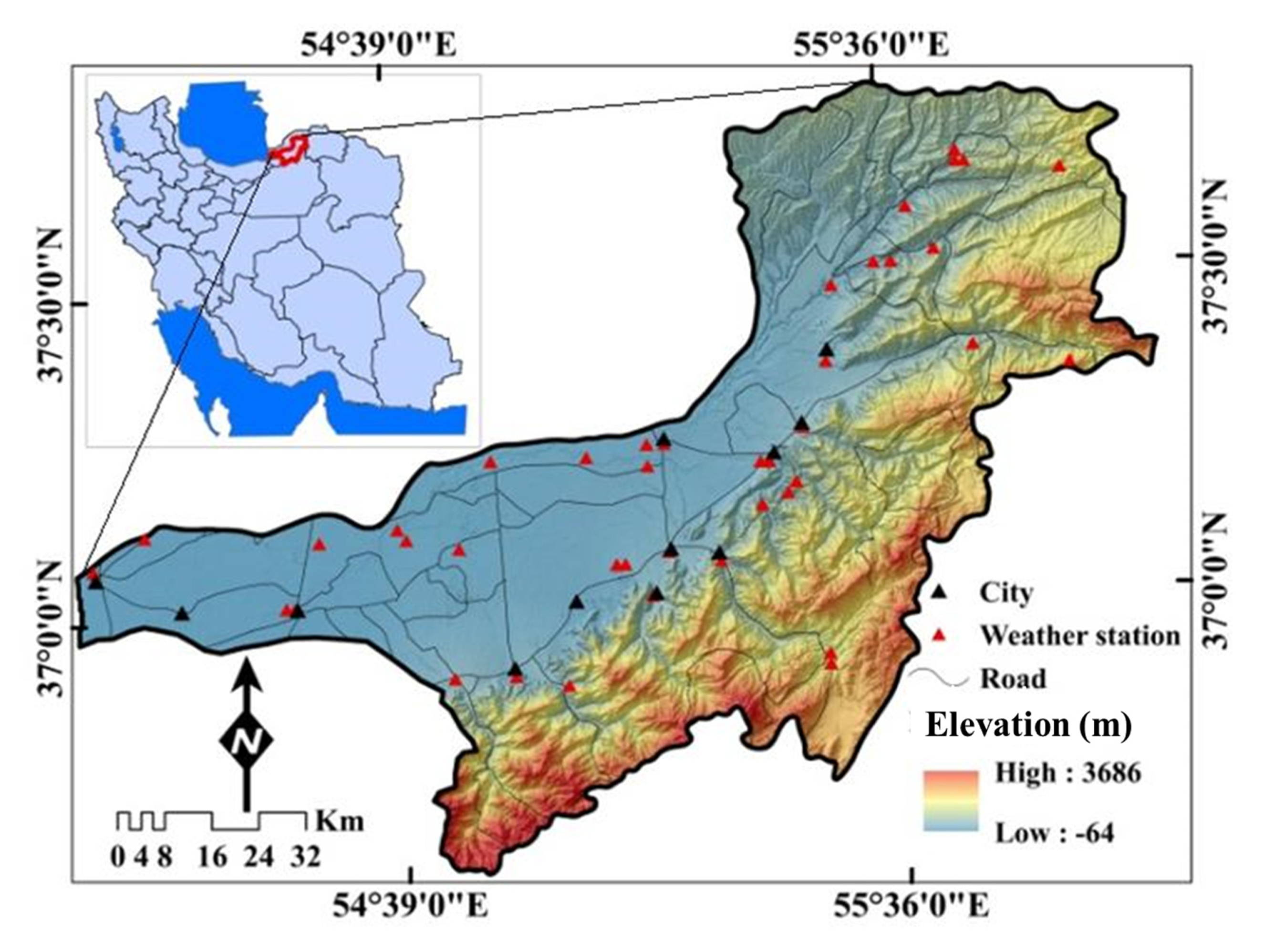
Figure 1. Location of the study area in Iran.
Remotesensing 12 03423 g001
Figure 2. Flowchart showing the methodology of the present work.
Remotesensing 12 03423 g002
Figure 3. Flood inventory map (a) flooded area in the city of Aqqala (b).
Remotesensing 12 03423 g003
Figure 4. InSAR data-processing procedure for DEM production.
Remotesensing 12 03423 g004
Figure 5. Flash flood conditioning factors, (a) slope (b) elevation, (c) plan curvature, (d) topographic wetness index (TWI), (e) topographic position index (TPI), (f) convergence index (CI), (g) stream power index (SPI), (h) distance to stream, (i) drainage density), (j) rainfall, (k) lithology, (l) soil type, (m) land use/land cover (LU/LC), (n) normalized difference vegetation index (NDVI).
Remotesensing 12 03423 g005aRemotesensing 12 03423 g005b
Figure 6. Flood susceptibility mapping, (a) J48 model, (b) MultiBoosting J48 (MJ48) model, (c) real AdaBoost J48 (RJ48) model, (d) Random Subspace J48 (RSJ48) model.
Remotesensing 12 03423 g006
Figure 7. Receiver operating characteristic (ROC) curves representing the accuracy of the flood susceptibility models (a) training dataset (success rate curve), (b) validation dataset (prediction rate curve).
Remotesensing 12 03423 g007
Figure 8. Trend of the frequency ratio (FR) in different models.
Remotesensing 12 03423 g008
Figure 9. Sensitivity analysis results from the percentage of contribution (PC) of each flood conditioning factor (FCF) in different models.
Remotesensing 12 03423 g009
Figure 10. Relative importance of flood conditioning factors using (a) AdaBoost model (b) boosted regression tree (BRT).
Remotesensing 12 03423 g010
Table 1. Multicollinearity test among flood conditioning factors.
FactorsCollinearity StatisticsFactorsCollinearity Statistics
VIFVIF
Land Use/Land Cover (LU/LC)1.330Distance to stream1.405
Soil type2.070Slope1.33
Elevation4.677TWI6.876
NDVI1.025Plan curvature 2.116
Lithology3.864TPI3.246
CI1.218Drainage density1.521
Rainfall1.523SPI4.21
Table 2. Spatial relationship between conditioning factors and floods by frequency ratio model.
FactorClassPixels in DomainFlood PixelsFR
No%No%
Elevation (m)<2874,346,42441.0526699.632.43
287–7842,168,21420.4810.370.02
784–13311,878,66717.74000
1331–19301,595,86815.07000
>1930599,2355.66000
Slope (°)<5.84,572,70943.2124591.762.12
5.8–14.21,907,63218.03217.870.44
14.2–22.61,985,05718.76000
22.6–32.51,468,31113.88000
>32.5648,3436.1310.370.06
plan curvature (100/m)Concave4,792,52845.2912747.571.05
Flat966,8519.142810.491.15
Convex4,822,67445.5711241.950.92
CI (100/m)<−52.9566,7395.422810.491.94
−52.9–−16.071,913,69318.296323.601.29
−16.07–14.55,483,51652.429736.330.69
14.5–50.52,040,04819.507026.221.34
>50.5456,9894.3793.370.77
SPI<8.872,478,65023.6411844.531.88
8.87–10.913,180,54730.338833.211.09
10.91–12.83,156,93130.104115.470.51
12.8–15.71,367,21513.0493.400.26
>15.7303,8412.9093.401.17
TPI<−10.98428,5834.0520.750.18
−10.98–−3.711,287,28912.1672.620.22
−3.71–2.346,565,37862.0424089.891.45
2.34–9.621,761,34916.64186.740.41
>9.62539,4525.10000
TWI<5.074,230,75639.98259.360.23
5.07–7.494047,82438.2515256.931.49
7.49–11.081,859,41717.577427.721.58
>11.08444,0554.20165.991.43
Drainage density (km/km2)<0.332,292,94621.672910.860.50
0.33–0.513,948,80437.329134.080.91
0.51–0.72,702,06825.538632.211.26
>0.71,638,25315.486122.851.48
Dis to stream (m)<1001,092,47210.329836.703.56
100–200930,6588.796423.972.73
200–300947,9408.963312.361.38
300–4007774287.35186.740.92
>4006,833,57364.585420.220.31
Rainfall (mm)<419.72,055,06819.446423.971.23
419.7–547.82,772,85026.2315156.552.16
547.8–682.62,365,87322.38269.740.44
682.6–820.61,890,89117.88269.740.54
>820.61,488,16914.08000
LU/LCForest3,185,82030.1310.370.01
Agriculture4,003,02437.8620074.911.98
Residential94,5510.892810.4911.73
Orchard171,8491.63000
Bare land89960.09000
Dry farming966,2379.1451.870.20
Rangeland1,954,19718.4841.500.08
Wood land139,0291.31000
Water/Wetland50,2320.482910.8622.86
LithologyCm, Cl491,6824.64000
Dp, DCkh593,5735.61000
Ekh, E1m74,8100.71000
Jsc, Jd, Jl, Jmz, Jch1,339,79712.65000
Kat, Ksn, Ksr, Ku, Kad-ab, Kl, K, Ktr743,5457.02000
Murm, Murmg90,5370.86000
PlQc, Pz, pC-C, Pr, Pz1a.bv, Pd, pCmt2, Plc, P576,3005.44000
Qsw, Qft2, Qm, Qft1, Qs, d, Qal605726157.212671001.75
TRe, TRe2, TRJs620,2055.86000
NDVI< 0.2016,200,34958.7723487.641.49
0.201–0.3691,538,52014.583011.240.77
> 0.3692,812,21326.6531.120.04
Soil typeRock Outcrops/Entisols1,453,17013.7310.370.03
Rock Outcrops/Inceptisols229,9332.17000
Salt Flats22,3310.21000
Alfisols1,792,75416.94000
Aridisols910,8118.615018.732.18
Inceptisols1,262,79311.93000
Mollisols4,908,83346.3921680.901.74
Table 3. Percentage of area under susceptibility classes in different machine learning models.
Flood Susceptibility ClassesJ48MJ48RJ48RSJ48
Very high18.67%24.60%16.239.21%
High 29.13%4.13%2.56%9.54%
Moderate 0.16%5.45%1.53%20.98%
Low 46.63%3.02%3.31%11.55%
Very low5.39%62.81%76.38%48.72%
Table 4. Values of efficiency (E), true skill statistic (TSS), sensitivity, and root mean square error (RMSE).
CriteriaValidation DatasetTraining Dataset
J48MJ48RJ48RSJ48J48MJ48RJ48RSJ48
TN1009590101221206217221
FP1594940232831
FN1823281746615046
TP103109114109227244239236
TPR0.850.830.800.870.830.800.830.84
FPR0.130.090.040.080.150.100.110.12
Efficiency0.860.860.860.890.840.840.850.86
TSS0.720.740.760.780.680.700.710.71
Sensitivity0.850.830.800.870.830.800.830.84
RMSE0.330.350.390.30.350.40.340.33
AUC0.8710.9290.8930.9510.8500.8890.9060.931
Table 5. Sensitivity analysis results from the percentage of contribution (PC) of each conditioning factor in different models.
Models
Factors
J48RJ48RSJ48MJ48
Elevation18.516.52116.5
Distance to stream14.413.416.913.4
NDVI11.59.513.259.5
Slope8.57.510.257.5
LU/LC7.55.58.255.5
Rainfall5.54.757.754.75
TWI3.7534.53
SPI3.22.453.952.45
Drainage density2.71.954.21.95
TPI2.251.53.751.5
Lithology1.751.253.51.25
Plan curvature1.450.73.250.7
Convergence index0.750.52.250.5
Soil type0.50.251.50.25
Publisher’s Note: MDPI stays neutral with regard to jurisdictional claims in published maps and institutional affiliations.