Snow Depth Variations in Svalbard Derived from GNSS Interferometric Reflectometry

 , ,
, ,  ,
,
Abstract
1. Introduction
2. Data and Methods
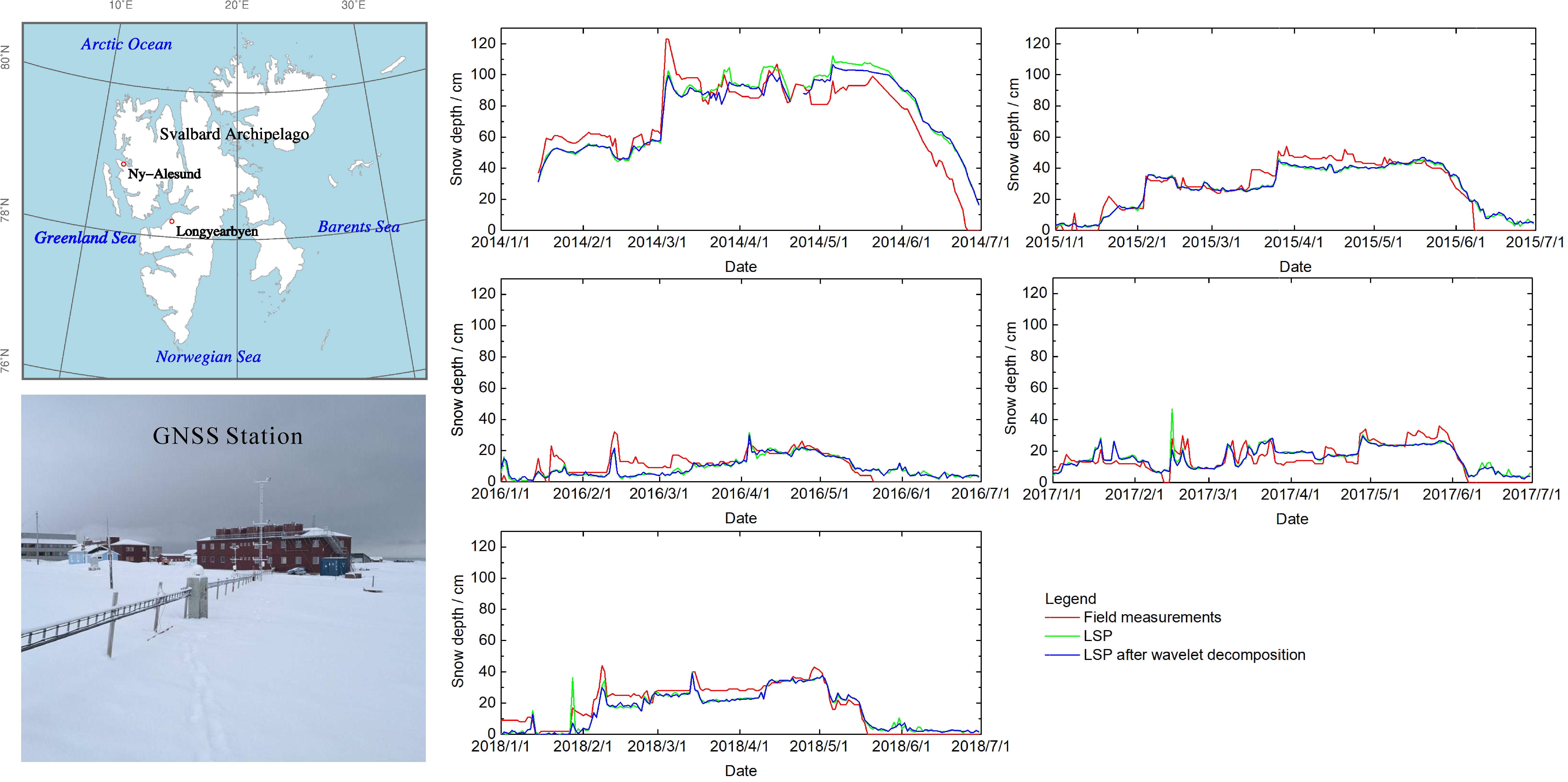
2.1. Data
2.2. Method
2.2.1. Approach Based on LSP Spectral Analysis
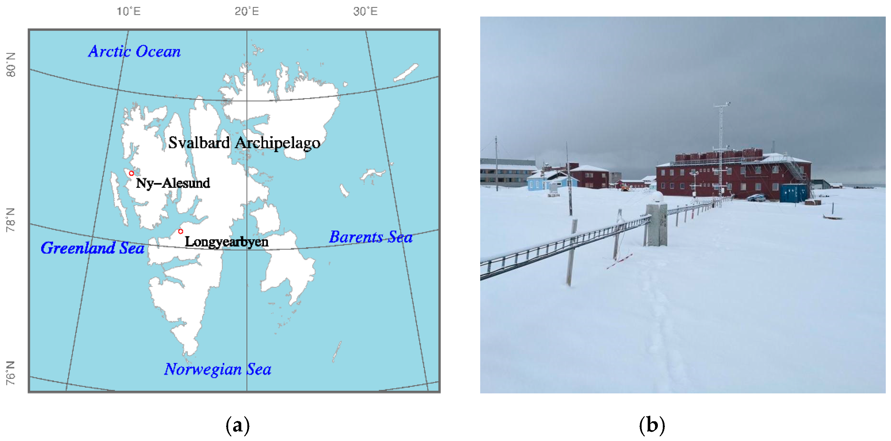
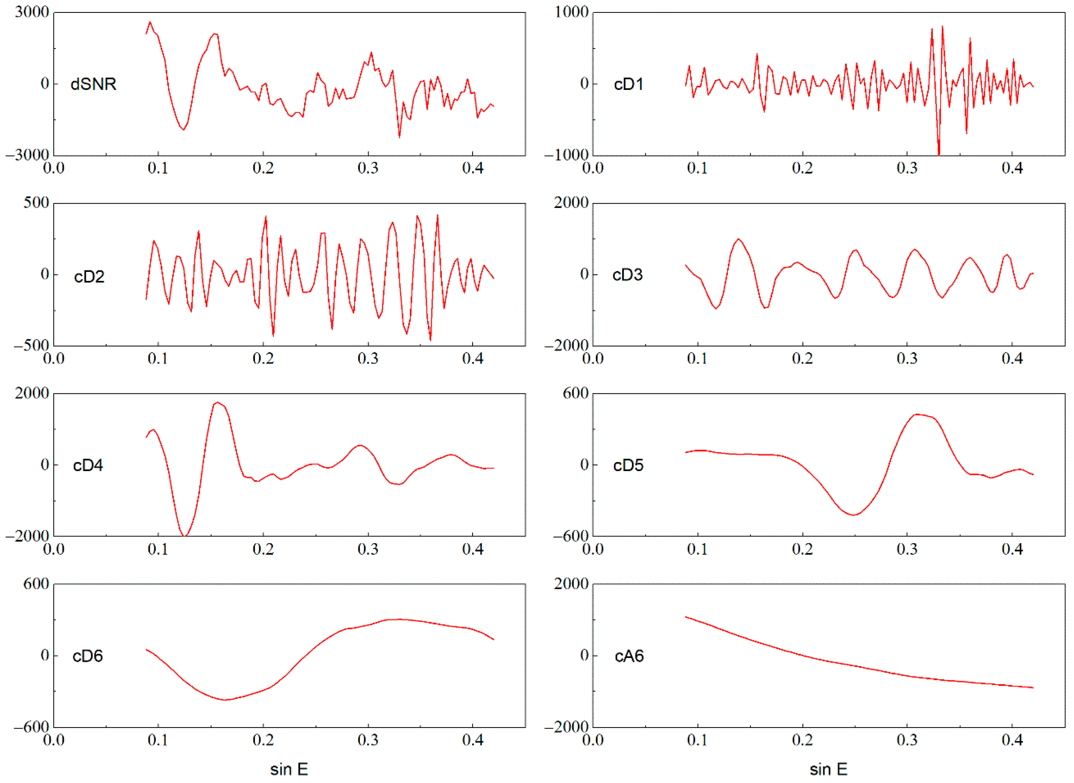
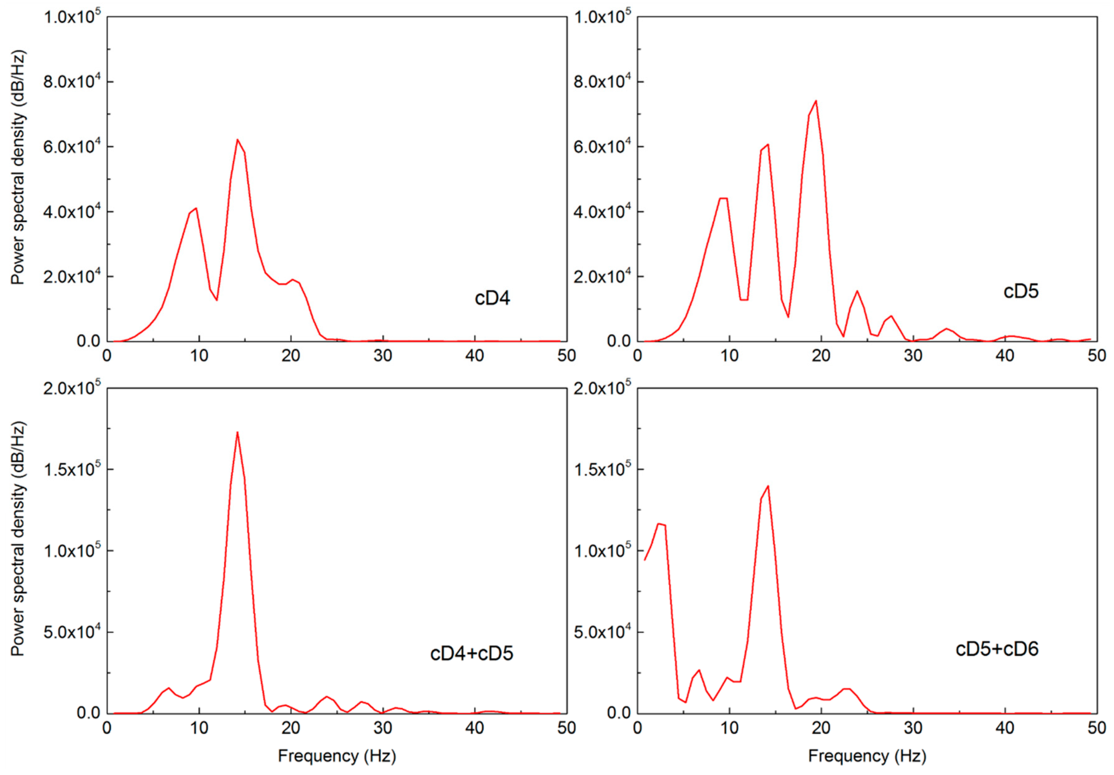
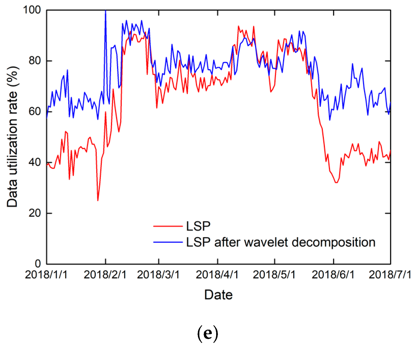
2.2.2. Improved Approach Based on Wavelet Analysis
3. Results and Discussion
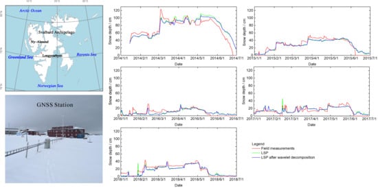
3.1. Daily Averaged Snow Depths over 5 Years
3.2. Performance of the Improved Approach
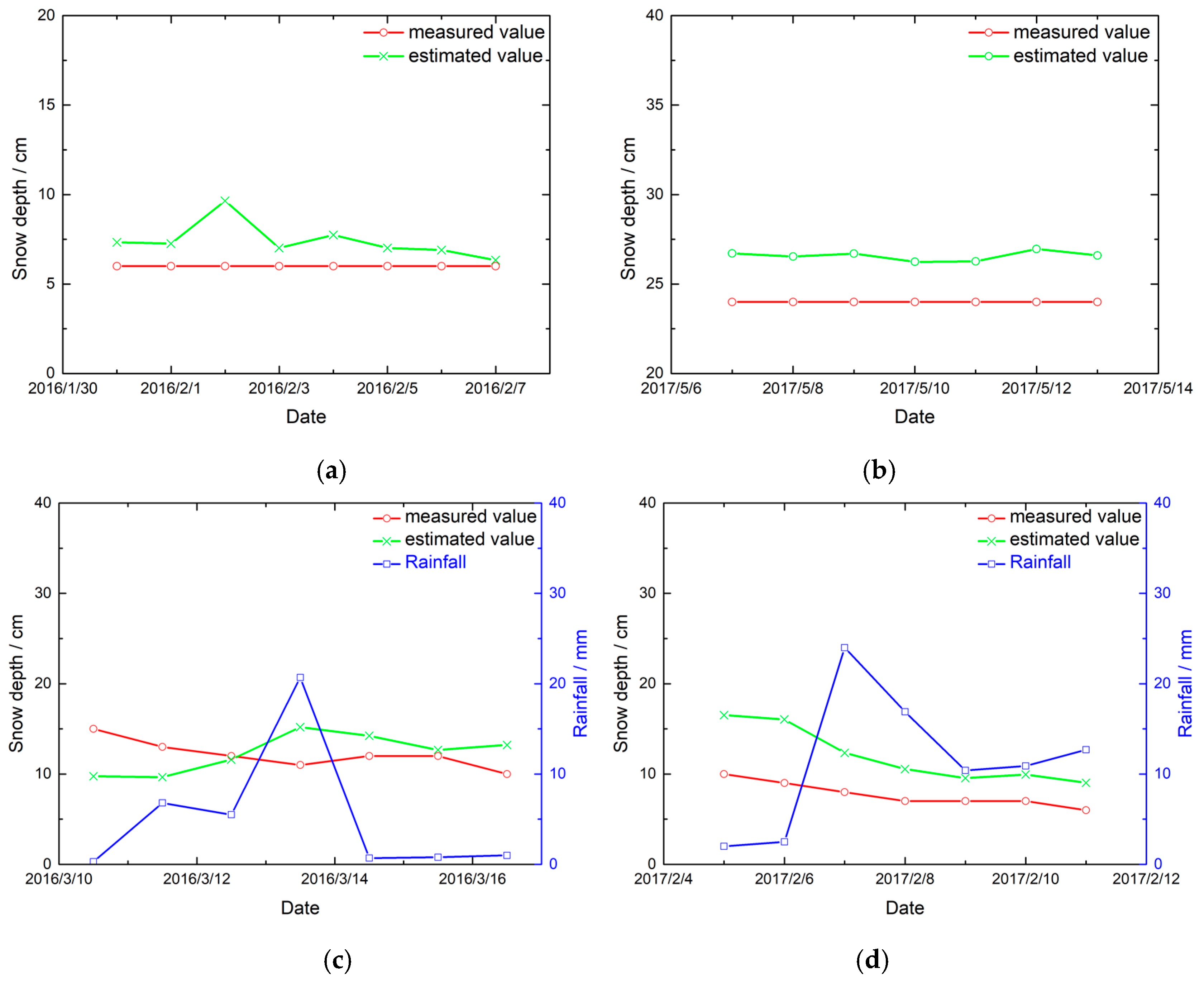
3.3. Effects of Snow-Surface Characteristics on Estimated Snow Depth
3.4. Effects of Rainfall on Estimated Snow Depth
4. Conclusions
Author Contributions
Funding
Acknowledgments
Conflicts of Interest
References
- Box, J.E.; Colgan, W.T.; Christensen, T.R.; Schmidt, N.M.; Lund, M.; Parmentier, F.-J.W.; Brown, R.; Bhatt, U.S.; Euskirchen, E.S.; Romanovsky, V.E.; et al. Key indicators of Arctic climate change: 1971–2017. Environ. Res. Lett. 2019, 14, 045010. [Google Scholar] [CrossRef]
- Ai, S.; Ding, X.; An, J.; Lin, G.; Wang, Z.; Yan, M. Discovery of the Fastest Ice Flow along the Central Flow Line of Austre Lovénbreen, a Poly-thermal Valley Glacier in Svalbard. Remote Sens. 2019, 11, 1488. [Google Scholar] [CrossRef]
- Bruland, O.; Sand, K.; Killingtveit, Å. Snow Distribution at a High Arctic Site at Svalbard. Hydrol. Res. 2001, 32, 1–12. [Google Scholar] [CrossRef]
- Bokhorst, S.; Pedersen, S.H.; Brucker, L.; Anisimov, O.; Bjerke, J.W.; Brown, R.D.; Ehrich, D.; Essery, R.L.H.; Heilig, A.; Ingvander, S.; et al. Changing Arctic snow cover: A review of recent developments and assessment of future needs for observations, modelling, and impacts. Ambio 2016, 45, 516–537. [Google Scholar] [CrossRef] [PubMed]
- Zhu, Y.; Shen, F. Snow Depth Determination Based on GNSS-IR. In Proceedings of the China Satellite Navigation Conference (CSNC), Beijing, China, 22–25 May 2019; pp. 98–105. [Google Scholar]
- Botteron, C.; Dawes, N.; Leclère, J.; Skaloud, J.; Weijs, S.V.; Farine, P.-A. Soil Moisture & Snow Properties Determination with GNSS in Alpine Environments: Challenges, Status, and Perspectives. Remote Sens. 2013, 5, 3516–3543. [Google Scholar]
- Komjathy, A.; Zavorotny, V.; Axelrad, P.; Born, G.; Garrison, J. Gps Signal Scattering From Sea Surface: Comparison Between Experimental Data And Theoretical Model. In Proceedings of the Fifth International Conference on Remote Sensing for Mar. and Coastal Environments, San Diego, CA, USA, 5–7 October 1998. [Google Scholar]
- Zavorotny, V.; Larson, K.; Braun, J.; Small, E.; Gutmann, E.; Bilich, A. A Physical Model for GPS Multipath Caused by Land Reflections: Toward Bare Soil Moisture Retrievals. IEEE J. Sel. Top. Appl. Earth Obs. Remote Sens. 2010, 3, 100–110. [Google Scholar] [CrossRef]
- Boniface, K.; Walpersdorf, A.; Guyomarc’h, G.; Deliot, Y.; Karbou, F.; Vionnet, V.; Nievinski, F. GNSS reflectometry measurement of snow depth and soil moisture in the French Alps. In Proceedings of the 2015 IEEE International Geoscience and Remote Sensing Symposium (IGARSS), Milan, Italy, 26–31 July 2015; pp. 5205–5207. [Google Scholar]
- Jacobson, M. Dielectric-Covered Ground Reflectors in GPS Multipath Reception—Theory and Measurement. Geosci. Remote Sens. Lett. IEEE 2008, 5, 396–399. [Google Scholar] [CrossRef]
- Chen, Q.; Won, D.; Akos, D.M. Snow depth sensing using the GPS L2C signal with a dipole antenna. EURASIP J. Adv. Signal Process. 2014, 2014, 106. [Google Scholar] [CrossRef]
- Siegfried, M.R.; Medley, B.; Larson, K.M.; Fricker, H.A.; Tulaczyk, S. Snow accumulation variability on a West Antarctic ice stream observed with GPS reflectometry, 2007–2017. Geophys. Res. Lett. 2017, 44, 7808–7816. [Google Scholar] [CrossRef]
- Vey, S.; Guntner, A.; Wickert, J.; Blume, T.; Thoss, H.; Ramatschi, M. Monitoring Snow Depth by GNSS Reflectometry in Built-up Areas: A Case Study for Wettzell, Germany. IEEE J. Sel. Top. Appl. Earth Obs. Remote Sens. 2016, 9, 4809–4816. [Google Scholar] [CrossRef]
- Larson, K.M.; Gutmann, E.D.; Zavorotny, V.U.; Braun, J.J.; Williams, M.W.; Nievinski, F.G. Can we measure snow depth with GPS receivers? Geophys. Res. Lett. 2009, 36. [Google Scholar] [CrossRef]
- Larson, K.M.; Small, E.E. Estimation of Snow Depth Using L1 GPS Signal-to-Noise Ratio Data. IEEE J. Sel. Top. Appl. Earth Obs. Remote Sens. 2016, 9, 4802–4808. [Google Scholar] [CrossRef]
- Jacobson, M. Inferring Snow Water Equivalent for a Snow-Covered Ground Reflector Using GPS Multipath Signals. Remote Sens. 2010, 2, 2426–2441. [Google Scholar] [CrossRef]
- Larson, K.M.; Nievinski, F.G. GPS snow sensing: Results from the EarthScope Plate Boundary Observatory. GPS Solut. 2013, 17, 41–52. [Google Scholar] [CrossRef]
- Nievinski, F.G.; Larson, K.M. Inverse Modeling of GPS Multipath for Snow Depth Estimation-Part I: Formulation and Simulations. IEEE Trans. Geosci. Remote Sens. 2014, 52, 6555–6563. [Google Scholar] [CrossRef]
- Tabibi, S.; Geremia-Nievinski, F.; van Dam, T. Statistical Comparison and Combination of GPS, GLONASS, and Multi-GNSS Multipath Reflectometry Applied to Snow Depth Retrieval. IEEE Trans. Geosci. Remote Sens. 2017, 55, 3773–3785. [Google Scholar] [CrossRef]
- Wang, Z.; Liu, Z.; An, J.; Lin, G. Snow depth detection and error analysis derived from SNR of GPS and BDS. Acta Geod. Cartogr. Sin. 2018, 47, 8–16. [Google Scholar]
- Durand, M.; Rivera, A.; Geremia-Nievinski, F.; Lenzano, M.G.; Monico, J.F.G.; Paredes, P.; Lenzano, L. GPS reflectometry study detecting snow height changes in the Southern Patagonia Icefield. Cold Reg. Sci. Technol. 2019, 166, 102840. [Google Scholar] [CrossRef]
- Wei, H.; He, X.; Feng, Y.; Jin, S.; Shen, F. Snow Depth Estimation on Slopes Using GPS-Interferometric Reflectometry. Sensors 2019, 19, 4994. [Google Scholar] [CrossRef]
- Ozeki, M.; Heki, K. GPS snow depth meter with geometry-free linear combinations of carrier phases. J. Geod. 2012, 86, 209–219. [Google Scholar] [CrossRef]
- Jin, S.; Najibi, N. Sensing snow height and surface temperature variations in Greenland from GPS reflected signals. Adv. Space Res. 2014, 53, 1623–1633. [Google Scholar] [CrossRef]
- Yu, K.; Wang, S.; Li, Y.; Chang, X.; Li, J. Snow Depth Estimation with GNSS-R Dual Receiver Observation. Remote Sens. 2019, 11, 2056. [Google Scholar] [CrossRef]
- Lomb, N.R. Least-squares frequency analysis of unequally spaced data. Astrophys. Space Sci. 1976, 39, 447–462. [Google Scholar] [CrossRef]
- Scargle, J.D. Studies in astronomical time series analysis. II—Statistical aspects of spectral analysis of unevenly spaced data. Astrophys. J. 1982, 263, 835. [Google Scholar] [CrossRef]
- Wang, X.; Zhang, Q.; Zhang, S. Water levels measured with SNR using wavelet decomposition and Lomb–Scargle periodogram. GPS Solut. 2018, 22. [Google Scholar] [CrossRef]
- Bilich, A.; Larson, K.M. Mapping the GPS multipath environment using the signal-to-noise ratio (SNR). Radio Sci. 2007, 42, RS6003. [Google Scholar] [CrossRef]
- Grossmann, A.J. Decomposition of Hardy Functions into Square Integrable Wavelets of Constant Shape. Soc. Ind. Appl. Math. 1984, 4, 723–736. [Google Scholar] [CrossRef]
- Mallat, S.G. A Theory for Multiresolution Signal Decomposition: The Wavelet Representation. IEEE Trans. Pattern Anal. Mach. Intell. 1989, 11, 674–693. [Google Scholar] [CrossRef]
- Daubechies, I. Ten Lectures on Wavelets; Society for Industrial and Applied Mathematics: Philadelphia, PA, USA, 1992. [Google Scholar]
- Gutmann, E.D.; Larson, K.M.; Williams, M.W.; Nievinski, F.G.; Zavorotny, V. Snow measurement by GPS interferometric reflectometry: An evaluation at Niwot Ridge, Colorado. Hydrol. Process. 2012, 26, 2951–2961. [Google Scholar] [CrossRef]
- Armstrong, J.S.; Collopy, F. Error measures for generalizing about forecasting methods: Empirical comparisons. Int. J. Forecast. 1992, 8, 69–80. [Google Scholar] [CrossRef]
- Willmott, C.J.; Matsuura, K. On the use of dimensioned measures of error to evaluate the performance of spatial interpolators. Int. J. Geogr. Inf. Sci. 2006, 20, 89–102. [Google Scholar] [CrossRef]
- Shiffler, R.E.; Harsha, P.D. Upper and Lower Bounds for the Sample Standard Deviation. Teach. Stat. 1980, 2, 84–86. [Google Scholar] [CrossRef]
- Henkel, P.; Koch, F.; Appel, F.; Bach, H.; Prasch, M.; Schmid, L.; Schweizer, J.; Mauser, W. Snow Water Equivalent of Dry Snow Derived From GNSS Carrier Phases. IEEE Trans. Geosci. Remote Sens. 2018, 56, 3561–3572. [Google Scholar] [CrossRef]
- Najibi, N.; Jin, S.; Wu, X. Validating the Variability of Snow Accumulation and Melting From GPS-Reflected Signals: Forward Modeling. IEEE Trans. Antennas Propag. 2015, 63, 2646–2654. [Google Scholar] [CrossRef]
- Koch, F.; Henkel, P.; Appel, F.; Schmid, L.; Bach, H.; Lamm, M.; Prasch, M.; Schweizer, J.; Mauser, W. Retrieval of Snow Water Equivalent, Liquid Water Content, and Snow Height of Dry and Wet Snow by Combining GPS Signal Attenuation and Time Delay. Water Resour. Res. 2019, 55, 4465–4487. [Google Scholar] [CrossRef]
Publisher’s Note: MDPI stays neutral with regard to jurisdictional claims in published maps and institutional affiliations. |


| Year | STD (cm) | MAE (cm) | RMSE (cm) | |||
|---|---|---|---|---|---|---|
| LSP | LSP after Wavelet Decomposition | LSP | LSP after Wavelet Decomposition | LSP | LSP after Wavelet Decomposition | |
| 2014 | 8.42 | 7.90 | 11.32 | 10.88 | 15.54 | 15.32 |
| 2015 | 6.08 | 6.14 | 4.26 | 4.34 | 5.52 | 5.62 |
| 2016 | 7.03 | 7.12 | 4.06 | 4.07 | 5.41 | 5.44 |
| 2017 | 6.74 | 6.32 | 4.30 | 4.14 | 5.46 | 5.12 |
| 2018 | 7.37 | 6.51 | 4.69 | 4.44 | 5.67 | 5.34 |
| mean | 7.13 | 6.80 | 5.72 | 5.57 | 7.52 | 7.37 |
| 2014 | 2015 | 2016 | 2017 | 2018 | Mean | |
|---|---|---|---|---|---|---|
| LSP | 78.66% | 81.80% | 57.94% | 78.77% | 63.72% | 72.18% |
| LSP after wavelet decomposition | 83.74% | 85.05% | 75.59% | 84.68% | 75.60% | 80.94% |
| Year | Snow-Accumulation Stage | Snow-Ablation Stage | Snow-Stabilization Stage | ||||
|---|---|---|---|---|---|---|---|
| LSP | LSP after Wavelet Decomposition | LSP | LSP after Wavelet Decomposition | LSP | LSP after Wavelet Decomposition | ||
| MAE (cm) | 2014 | 7.06 | 4.66 | 9.85 | 9.05 | 4.98 | 4.97 |
| 2015 | 3.76 | 3.95 | 3.54 | 3.25 | 3.86 | 3.25 | |
| 2016 | 6.13 | 5.78 | 5.67 | 4.85 | 2.74 | 2.63 | |
| 2017 | 6.31 | 4.65 | 4.20 | 3.77 | 4.73 | 4.33 | |
| 2018 | 6.23 | 4.82 | 5.12 | 4.65 | 2.36 | 2.35 | |
| mean | 5.90 | 4.77 | 5.68 | 5.11 | 3.73 | 3.51 | |
| RMSE (cm) | 2014 | 8.58 | 5.70 | 11.18 | 10.37 | 5.34 | 5.17 |
| 2015 | 5.30 | 5.31 | 4.31 | 4.03 | 3.93 | 3.38 | |
| 2016 | 8.51 | 8.03 | 7.54 | 7.11 | 3.69 | 3.49 | |
| 2017 | 8.64 | 5.04 | 6.43 | 4.99 | 5.06 | 4.03 | |
| 2018 | 8.40 | 5.93 | 5.69 | 5.18 | 2.77 | 2.83 | |
| mean | 7.89 | 6.00 | 7.03 | 6.34 | 4.16 | 3.78 | |
| Year | MAE (cm) | RMSE (cm) | ||
|---|---|---|---|---|
| No Rainfall | Rainfall | No Rainfall | Rainfall | |
| 2014 | 4.45 | 11.81 | 4.41 | 11.66 |
| 2015 | 1.32 | 4.41 | 1.43 | 4.22 |
| 2016 | 1.40 | 2.76 | 1.68 | 3.21 |
| 2017 | 2.57 | 4.29 | 2.58 | 4.60 |
| 2018 | 0.71 | 4.16 | 0.81 | 4.31 |
| mean | 2.19 | 5.63 | 2.08 | 5.46 |
© 2020 by the authors. Licensee MDPI, Basel, Switzerland. This article is an open access article distributed under the terms and conditions of the Creative Commons Attribution (CC BY) license (http://creativecommons.org/licenses/by/4.0/).
Share and Cite
An, J.; Deng, P.; Zhang, B.; Liu, J.; Ai, S.; Wang, Z.; Yu, Q. Snow Depth Variations in Svalbard Derived from GNSS Interferometric Reflectometry. Remote Sens. 2020, 12, 3352. https://doi.org/10.3390/rs12203352
An J, Deng P, Zhang B, Liu J, Ai S, Wang Z, Yu Q. Snow Depth Variations in Svalbard Derived from GNSS Interferometric Reflectometry. Remote Sensing. 2020; 12(20):3352. https://doi.org/10.3390/rs12203352
Chicago/Turabian StyleAn, Jiachun, Pan Deng, Baojun Zhang, Jingbin Liu, Songtao Ai, Zemin Wang, and Qiuze Yu. 2020. "Snow Depth Variations in Svalbard Derived from GNSS Interferometric Reflectometry" Remote Sensing 12, no. 20: 3352. https://doi.org/10.3390/rs12203352
APA StyleAn, J., Deng, P., Zhang, B., Liu, J., Ai, S., Wang, Z., & Yu, Q. (2020). Snow Depth Variations in Svalbard Derived from GNSS Interferometric Reflectometry. Remote Sensing, 12(20), 3352. https://doi.org/10.3390/rs12203352