Exploring the Impact of Various Spectral Indices on Land Cover Change Detection Using Change Vector Analysis: A Case Study of Crete Island, Greece

Abstract

The main objective of this study was to explore the impact of various spectral indices on the performance of change vector analysis (CVA) for detecting the land cover changes on the island of Crete, Greece, between the last two decades (1999–2009 and 2009–2019). A set of such indices, namely, normalized difference vegetation index (NDVI), soil adjusted vegetation index (SAVI), albedo, bare soil index (BSI), tasseled cap greenness (TCG), and tasseled cap brightness (TCB), representing both the vegetation and soil conditions of the study area, were estimated on Landsat satellite images captured in 1999, 2009, and 2019. Change vector analysis was then applied for five different index combinations resulting to the relative change outputs. The evaluation of these outputs was performed towards detailed land cover maps produced by supervised classification of the aforementioned images. The results from the two examined periods revealed that the five index combinations provided promising performance results in terms of kappa index (with a range of 0.60–0.69) and overall accuracy (with a range of 0.86–0.96). Moreover, among the different combinations, the use of NDVI and albedo were found to provide superior results against the other combinations.

1. Introduction

Land cover plays a significant role in the terrestrial ecosystem biodiversity, water resources, climate system, and socio-economic sectors. The term “land cover” originally referred to the distribution and type of vegetation (e.g., cropland, forests) that covered a land’s surface [1]. However, nowadays, it is considered to describe the general biophysical state of the surface also providing information about other aspects of the land such as soils and water [1].

Changes in land cover caused by several natural and anthropogenic forces and represented by relative biophysical changes to the land surface have noticeable impacts on the quality of environmental and ecological systems. Therefore, land cover changes can constitute the main indicators of environmental/ecological change at different spatial and temporal scales. The detection and evaluation of these spatio-temporal changes has become a major priority for researchers and policy makers around the world over the last few decades [2].

In order to study land cover changes in a given region, it is necessary to have information that reflects its status at different times. Satellite remote sensing—most of the times, in combination with geographic information systems (GIS)—has been recognized as a powerful and cost-effective tool which can provide valuable multi-temporal information for detecting such changes. Due to the ability of satellites to cover, continuously and repeatedly, vast and inaccessible areas as well as the advancements in the quality (spatial resolution) of output imagery data, remote sensing-based techniques have been widely applied in numerous studies focusing on land cover change detection [3,4,5]. In terms of remote sensing, change detection is defined as the process in which temporal differences in the state of an object or phenomenon are identified [6]. Considering the imagery data processing approach, the change detection techniques can be divided into two main categories: (a) based on spectral classification of satellite images for each date; and (b) based on metric difference among satellite images of different dates or data products derived from their transformation.

The biophysical properties of land surface are mainly expressed as coverages by vegetation or bare soil. These properties can be measured by transformation-based data products such as vegetation and soil indices. Based on the degree of absorption/reflectance from the land surface in the different portions of electromagnetic spectrum (satellite bands), the indices represent the vegetation and soil conditions, respectively, for a given region, using a defined value range. The relationship between spectral indices and land cover change detection is well established resulting from their common examination in this kind of analyses [7,8,9].

Concerning the recent (within last decade) literature, several studies have focused on land cover change detection for various geographical settings in Greece, using remotely sensed techniques and data. It is worth mentioning that, in these studies, classification-based techniques have been selected to be applied. Among others, Dawson et al. [10] assessed the land cover of the Itanos area on the island of Crete and then detected its changes for the period 2013–2016. They carried out object-based image analysis to classify the land cover on high spatial resolution satellite imagery. Xystrakis et al. [11] mapped the land cover changes for different time intervals of the period 1945–2009 in Aetoloakarnania prefecture, central Greece. Also, in this case, an object-based image analysis allowed the multi-temporal classification of the land cover and, consecutively, the detection of changes for each time interval. Symeonakis [12] identified the land cover changes on the island of Lesvos for the period 1995–2007 by the classification of satellite imagery data. Furthermore, in a study by Kolios and Stylios [13], the land cover changes in the Preveza region for the period 2000–2009 were detected, examining several remotely sensed data along with the implementation of different traditional and modern classification techniques. Mallinis et al. [14] mapped land cover changes in Nestos delta (“Natura 2000” habitat site in northern Greece) by exploiting high spatial resolution satellite images. Maps created for separate time intervals over a total period of about 65 years contributed to the change detection.

The main purpose of this study was to explore the effect of various spectral indices on the implementation of a metric difference-based technique, known as change vector analysis (CVA), for detecting the land cover changes on the total extent of Crete Island during the decades 1999–2009 and 2009–2019. These indices were derived from satellite images from 1999, 2009, and 2019. Change vector analysis produced change results for each of the examined time periods presenting the magnitude and type of changes, respectively, based on five different index combinations. The most appropriate index combination for detecting the land cover changes in the study area was determined by an evaluation process resulting to the estimation of accuracy statistics (kappa index and overall accuracy).

2. Materials and Methods

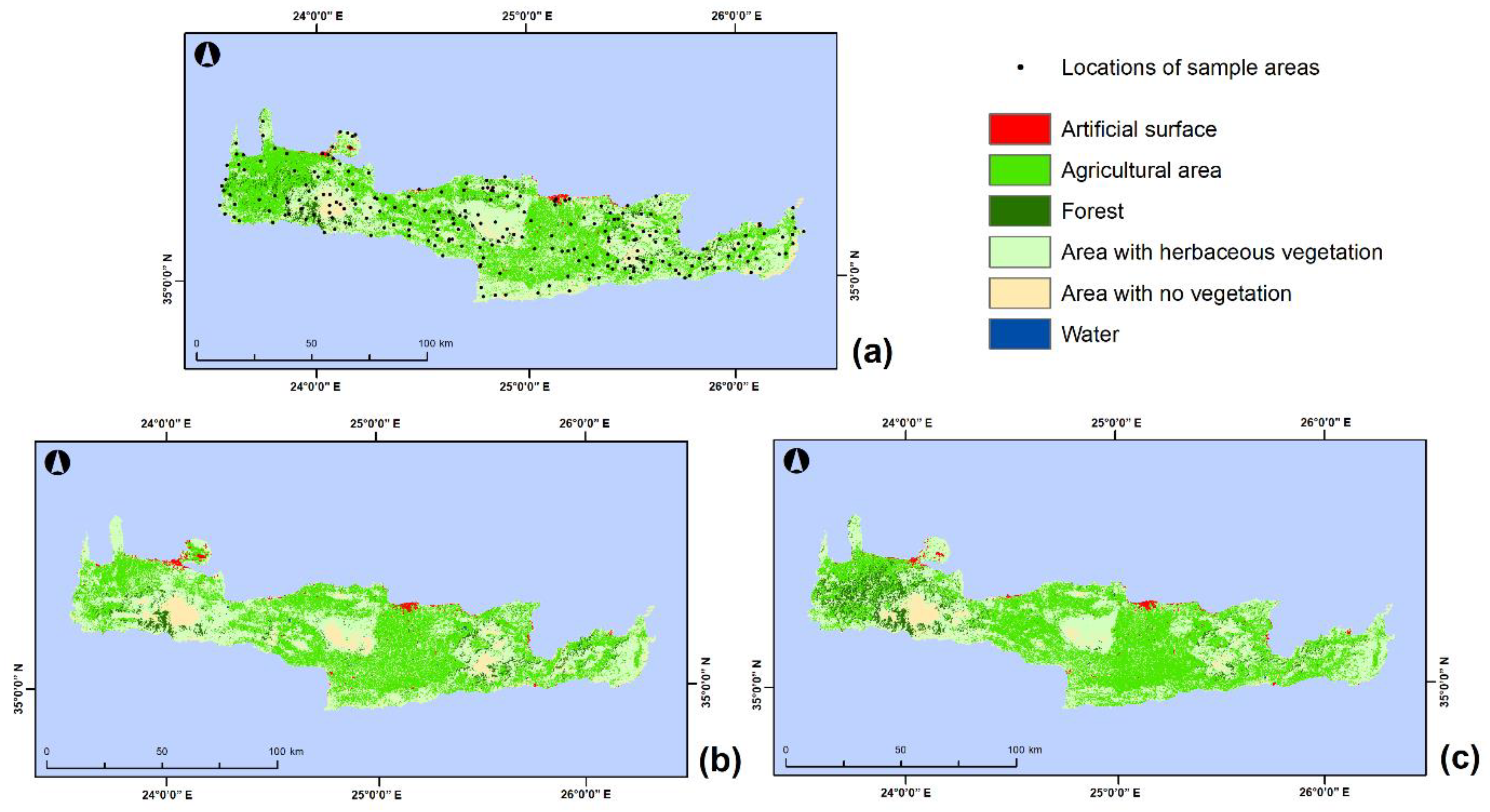
2.1. Study Area

The island of Crete is located in the southern part of Greece (Figure 1), having a distance of 160 km from the Greek mainland. It separates the Aegean Sea from the Libyan Sea and is surrounded by numerous smaller islands including Gavdos, the southernmost Greek and European border. With an extent of 8257 km² (about 6% of the total area of Greece), length of 260 km, and width ranging from 12 km to 57 km, Crete constitutes the largest Greek island and the fifth largest in the Mediterranean region. Administratively, it is divided into four prefectures from west to east: Chania, Rethymno, Heraklion, and Lasithi (Figure 1). According to the official 2011 census [15] held by the Hellenic Statistical Authority (ELSTAT), Crete is the most populated Greek island with 623,065 inhabitants (5.8% of the total population of Greece). As a result of significant increase in urban and touristic activities over the last two decades, the majority of them are concentrated in coastal areas [16].

The topography of Crete follows the typical Greek landscape consisting mainly of mountainous terrain (with a mean elevation at 460 m). A great number of landforms (caves, plateaus, etc.) have developed among its mountains. The variable morphology as well as the position of the island between the Mediterranean and North African climatic zones have played an important role in its climate. In general, it is considered mild with warm and dry summers and slightly cold and humid winters. The average temperature is 10 ℃ in the winter season and 30 ℃ in the summer season. The mean annual precipitation is estimated to be 750 mm, presenting strong spatial and temporal differences. Specifically, more than 40% occurs in the winter months ranging from 440 mm in the east to 2188 mm in the west [17].

Geologically, the island is composed of pre-Alpine and Alpine carbonate rocks, and Neogene and Quaternary (alluvial) sediments. The carbonate rocks, such as limestones, marbles, and dolomites, constitute the dominant geological formations covering more than 30% of the total area. Since these formations expedite water penetration, the region is characterized by limited surface waters.

Grasslands and permanent crops of olives, vines, and citrus cover most of the study area. Heterogeneous croplands or fields mixed with natural vegetation also make their appearance over a significant part of the island. The extensive agricultural activity has caused a strong dependence of the island on groundwater sources [18].

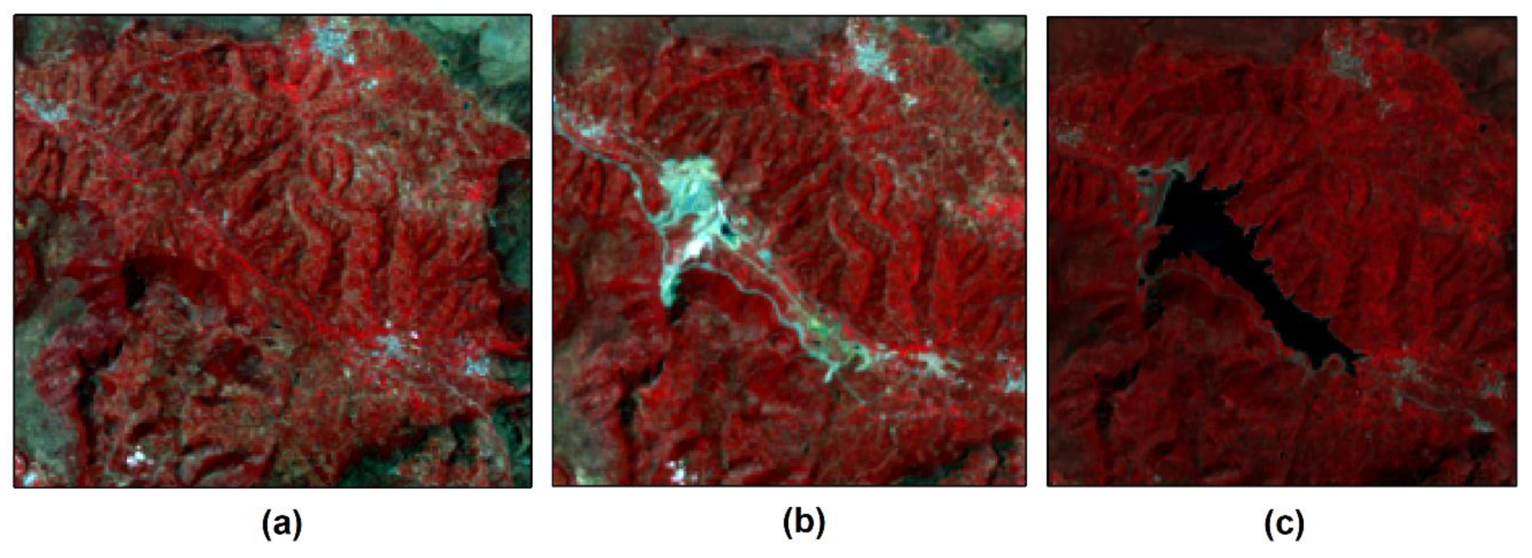
2.2. Satellite Imagery Data

Considering the relation between the examined time period of 1999–2019 and the temporal availability of data, Landsat satellite images were selected to be analyzed in this study. In particular, multispectral imagery data acquired from the Landsat 5 thematic mapper (TM) in May 1999, Landsat 7 enhanced thematic mapper plus (ETM+) in May 2009, and Landsat 8 operational land imager (OLI) in May 2019 were used. The acquisition date selection mainly depended on the need for acquiring images: (a) from the peak of the vegetation growing season (from May to June) and (b) with no influence by cloud cover limitations. Due to the size of the study area, three image tiles with a spatial resolution of 30 m were provided by the United States Geological Survey (USGS) [19] for each date in order to build a cloudless image covering the total extent.

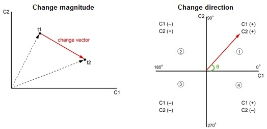
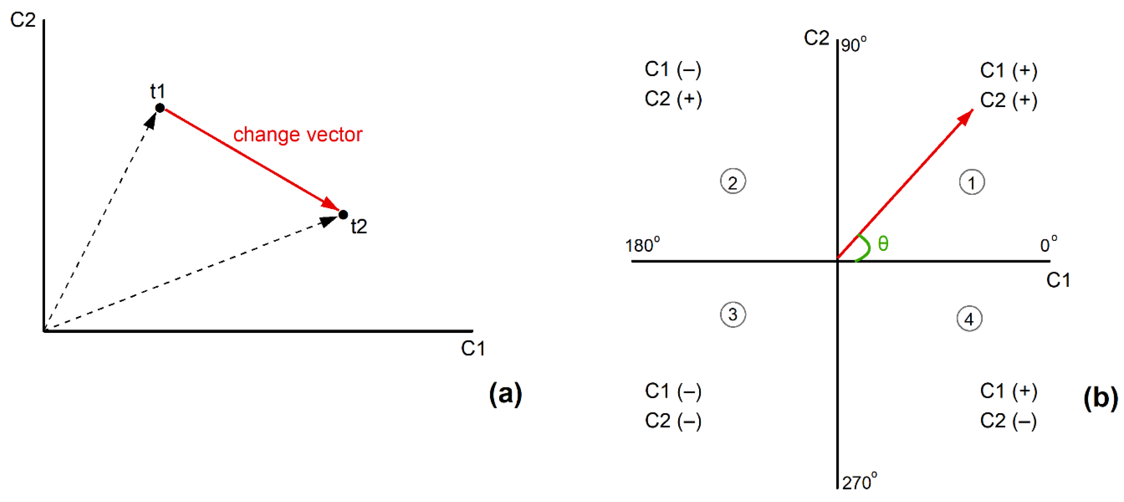
2.3. Change Vector Analysis

Change vector analysis, which has been widely used to study the spatio-temporal dynamics of land cover [20,21,22], is a change detection technique which presents the change as a vector in a multi-dimensional space. By examining the metric difference of input components that can be either original satellite (band) images or transformed data products of different dates, CVA enables pixel-by-pixel mapping of the magnitude and direction of the changes among the selected dates. The number of dimensions of the space is defined by the number (n) of components. In the case of using two components, the relative two-dimensional space can be represented by a Cartesian coordinate system with two axes (Figure 2). The change vector is formed by two points corresponding to the same pixel at two different dates [20]. The start point and finish point are considered to be the locations of pixel (with pixel values as coordinates) in the space of two components at these two dates.

The magnitude (ΔM) of the change between date 1 (t1) and date 2 (t2) is based on the length of change vector (Figure 2a) and is computed by the Euclidean distance as follows:

$$\Delta M = \sqrt{{\left({C1}_{t2} –{C1}_{t1}\right)}^2 + {\left({C2}_{t2 }–{C2}_{t1}\right)}^2}$$

(1)

where C1_t1 and C1_t2 are the pixel values in component 1 at dates 1 and 2, respectively, and C2_t1 and C2_t2 are the pixel values in component 2 at dates 1 and 2, respectively. A threshold, usually in terms of standard deviations, is defined for the magnitude values to distinguish between changed and unchanged parts of the study area [21].

The direction of the change is based on the angle (θ) of change vector (Figure 2b) indicating the type of change from one date to the other. The angle defines the quadrant and can be derived from Equation (2):

$$tan\theta =\frac{{C1}_{t2} –{C1}_{t1}}{{C2}_{t2} –{C2}_{t1}}$$

(2)

where tanθ is the tangent of angle θ. Since the number of quadrants is equal to 2n, the direction of the change is categorized as four quadrants (Figure 2b). The first quadrant (0°–90°) and the third quadrant (180°–270°) indicate an increase and decrease in both components, respectively. The second quadrant (90°–180°) and the fourth quadrant (270°–360°) indicate that one of the components increased and the other one decreased.

2.4. Land Cover Change Detection

2.4.1. Imagery Data Pre-Processing

The imagery data pre-processing was performed in ENVI (version 5.1) software and included the atmospheric and radiometric corrections as well as the mosaicking of the obtained Landsat image tiles. When using imagery data from different satellite sensors, acquired at different dates, the atmospheric and radiometric corrections are prerequisite for creating high-quality data that are less or not affected by atmospheric differences and variations due to the solar irradiance. Based on dark object subtraction approach [23] and radiometric rescaling coefficients [24], the result was the conversion of the pixel values of Landsat image tiles from original digital numbers into top-of-atmosphere (TOA) reflectance values. The corrected image tiles of each date were then mosaicked (as it was abovementioned) in order to build a full image covering the total extent of the study area.

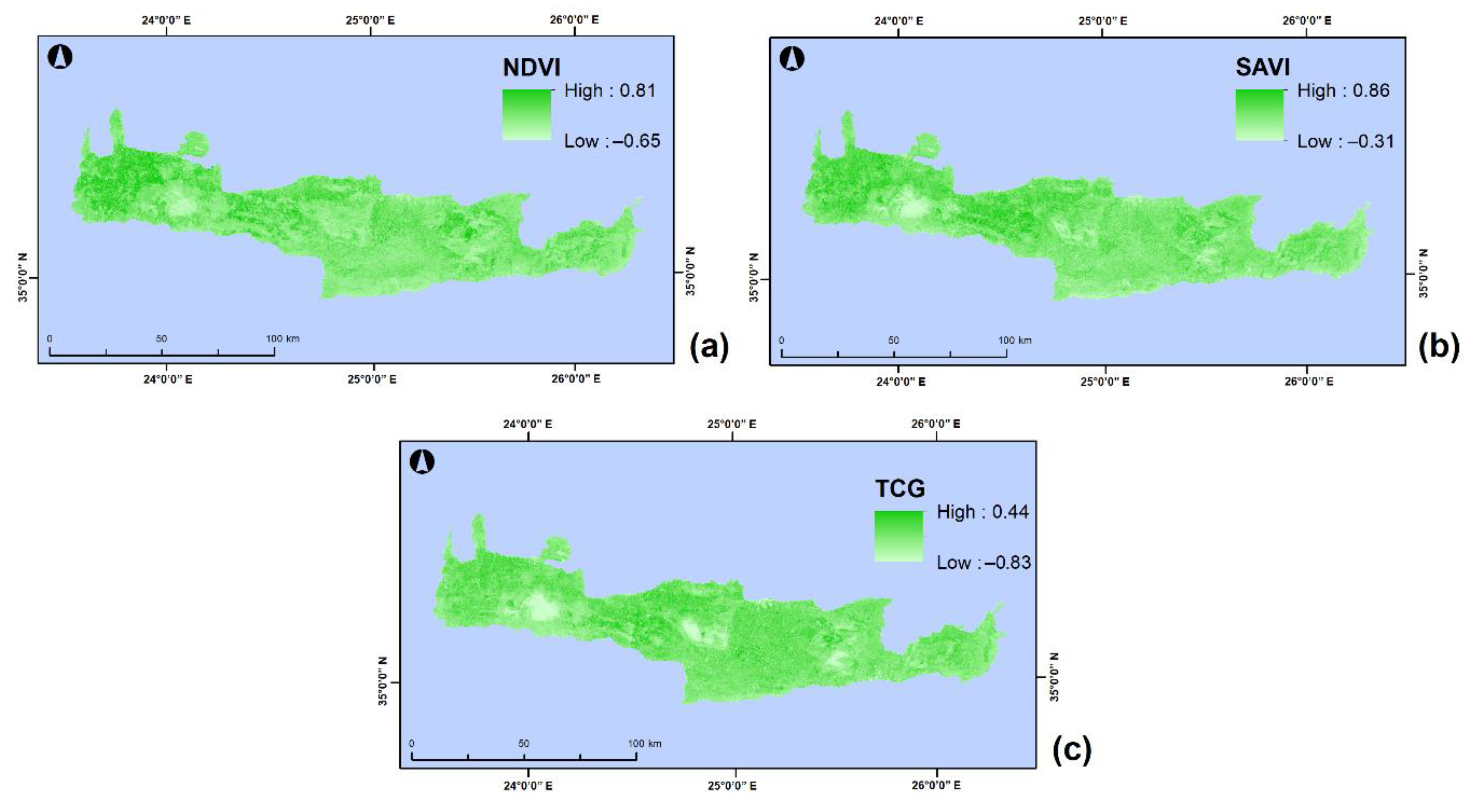
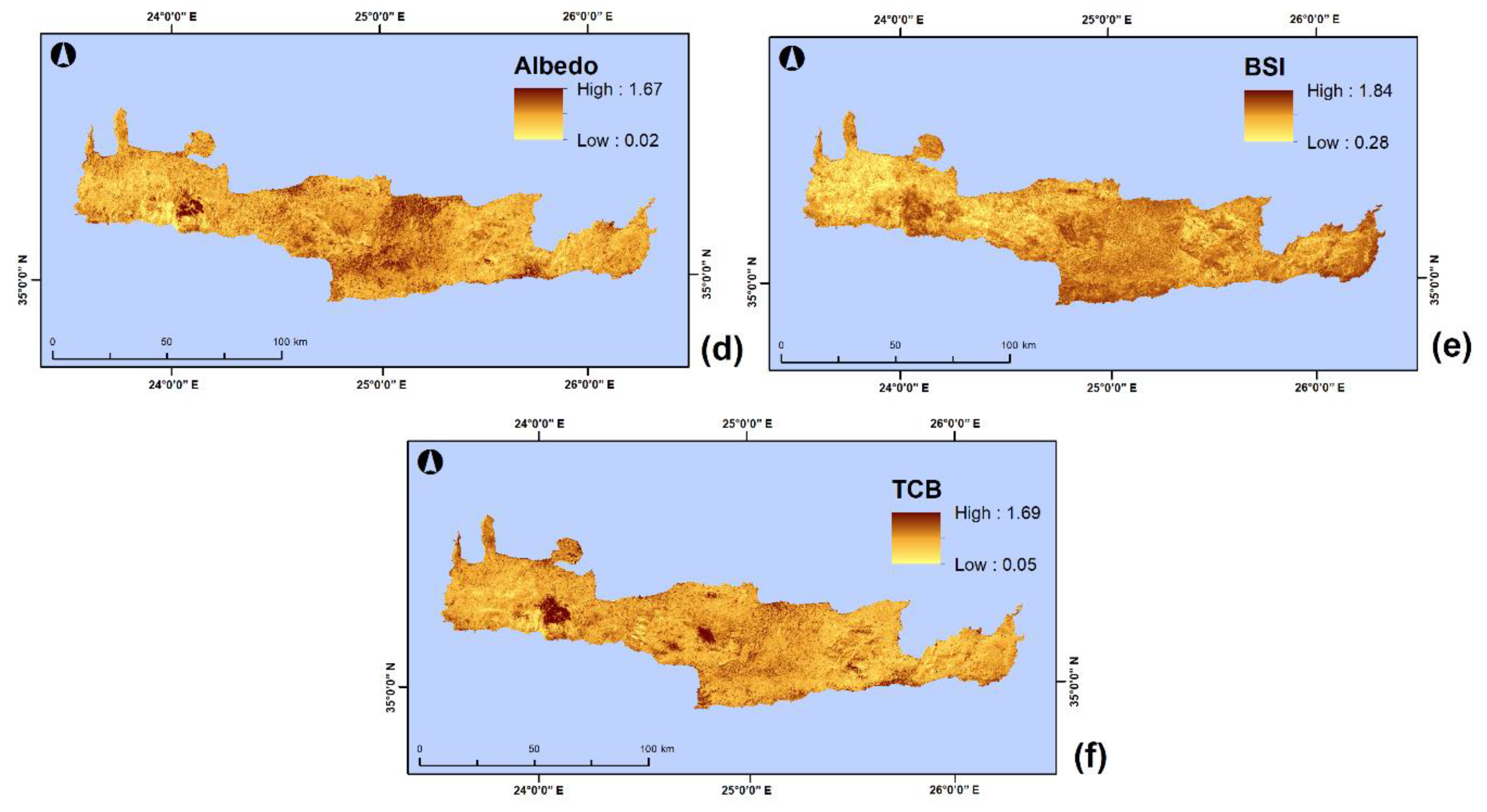
2.4.2. Preparation of Spectral Indices

The biophysical properties of a given region can be assessed by several spectral indices which are developed after processing of satellite imagery data. These indices are subdivided into two main types representing: (a) the vegetation conditions and (b) the soil conditions of the region. In total, six spectral indices were considered in this study including three vegetation indices, namely, normalized difference vegetation index (NDVI), soil adjusted vegetation index (SAVI), tasseled cap greenness (TCG), and three soil indices, namely, albedo, bare soil index (BSI), and tasseled cap brightness (TCB).

The NDVI is the most known and widely used index for vegetation density [25]. Among several relative parameters, it can be highly linked to the quantity of chlorophyll concentrated in leaves and the biomass productivity variations. The NDVI is calculated by the following Equation (3) [21]:

$$NDVI=\frac{{\rho }_{NIR}–{\rho }_{\mathit{RED}}}{{\rho }_{\mathit{NIR}}{+ \rho }_{\mathit{RED}}}$$

(3)

where ρ_NIR and ρ_RED are the reflectance values at the near-infrared and red visible bands, respectively, of the Landsat imagery data. The resulting values are bounded by a range between −1 and 1, indicating a lack of vegetation or dense vegetation, respectively.

The SAVI minimizes the soil influence on vegetation quantification by introducing a soil adjustment factor. It is computed in a range between –1 and 1 by the Equation (4) [26]:

$$\mathit{SAVI} =\left(\frac{{\rho }_{\mathit{NIR}}–{\rho }_{\mathit{RED}}}{{\rho }_{\mathit{NIR}}{+ \rho }_{\mathit{RED}}+ L}\right)\times \left(1 + L\right)$$

(4)

where L is the soil adjustment factor, commonly set at a 0.5 value.

Albedo reflects soil conditions, including soil moisture and soil exposure, based on the quantity of radiation energy absorbed by the land surface. It is estimated as follows [27]:

$$\mathit{Albedo} = 0.356{\rho }_{\mathit{BLUE}} + 0.130{\rho }_{\mathit{RED}} + 0.373{\rho }_{\mathit{NIR}} + 0.085{\rho }_{\mathit{SWIR}1}+ 0.072{\rho }_{\mathit{SWIR}2}–0.0018$$

(5)

where ρ_BLUE, ρ_SWIR1 and ρ_SWIR2 are the reflectance values at the blue visible, short-wave infrared 1, and short-wave infrared 2 bands, respectively, of the Landsat imagery data. In this study, albedo was estimated in a normalized form according to Reference [28]. The resulting values are bounded by a range between 0 and 2 indicating vegetation cover or barren land, respectively.

The BSI is mainly used to highlight the difference between agricultural and non-agricultural land due to the fact of its enhanced ability to identify bare soil and fallow lands. It is derived in a range between 0 and 2 from the equation [22]:

$$\mathit{BSI} =\left(\frac{\left({\rho }_{\mathit{RED}}{ + \rho }_{\mathit{SWIR}1}\right) –\left({\rho }_{\mathit{NIR}}{+ \rho }_{\mathit{BLUE}}\right)}{\left({\rho }_{\mathit{RED}}{ + \rho }_{\mathit{SWIR}1}\right) + \left({\rho }_{\mathit{NIR}}{+ \rho }_{\mathit{BLUE}}\right)}\right)+ 1$$

(6)

Tasseled cap (TC) is the transformation of imagery data into a number of components allowing better separability between vegetation and bare soil. Among the components, brightness and greenness are considered the most noticeable in terms of land cover. The TCG (with a range between –1 and 1) and TCB (with a range between 0 and 2) are defined on the basis of soil and vegetation, respectively, reflectance variations. Their TC transformation-based creation is achieved using fixed coefficients [29,30,31] in equations similar to Equation (5). As it is shown in

Table 1. Coefficients for tasseled cap greenness and brightness.

Satellite Sensor	Index	Bands
		BLUE	GREEN	RED	NEAR-INFRARED (NIR)	SHORT-WAVE INFRARED 1 (SWIR1)	SHORT-WAVE INFRARED 2 (SWIR2)
Landsat 5 TM	Greenness	–0.2848	–0.2435	–0.5436	0.7243	0.0840	–0.1800
	Brightness	0.3037	0.2793	0.4743	0.5585	0.5082	0.1863
Landsat 7 ETM+	Greenness	–0.3344	–0.3544	–0.4556	0.6966	–0.0242	–0.263
	Brightness	0.3561	0.3972	0.3904	0.6966	0.2286	0.1596
Landsat 8 OLI	Greenness	–0.2941	–0.243	–0.5424	0.7276	0.0713	–0.1608
	Brightness	0.3029	0.2786	0.4733	0.5599	0.5080	0.1872

, these coefficients are different for each of the Landsat sensors (TM, ETM+, and OLI) and corresponding bands.

By executing all the aforementioned equations in ArcGIS (version 10.6) software, the relative spectral indices were obtained for 1999, 2009, and 2019. An overview of these indices is presented for selected dates in Figure 3.

2.4.3. Implementation of CVA

In the present study, CVA was selected to be implemented for land cover change detection using five different combinations of the above spectral indices. In each implementation, a vegetation index as component 1 (C1) and a soil index as component 2 (C2) were considered resulting to the following combinations: NDVI–albedo, NDVI–BSI, SAVI–albedo, SAVI–BSI and TCG–TCB. This selection for the number of components led to the formation of a two-dimensional space and four directional quadrants as schematically described by Cartesian coordinate system in Figure 2.

By using Equation (1) in ArcGIS software, the magnitude of land cover changes in the study area was estimated for each of the examined index combinations and time periods. One standard deviation from the mean was determined as threshold to distinguish between change and no change [21,32]. In a similar manner, the level of change was determined as low and high, respectively. The change magnitude outputs for the periods of 1999–2009 and 2009–2019 are presented as maps categorized into three categories: “no change”, “low level change”, and “high level change”.

By using Equation (2), the change direction was then defined according to the angles of change vectors. Each of the four quadrants is related to a category representing the type of land cover changes in the study area. Therefore, the first category with an increase in both spectral indices represents biomass variation or moisture reduction. This category indicates areas with variations in the amount of biomass that can be associated with changes in agricultural areas such as crop substitution or different phenological stages in the agricultural cycle [20]. The second category with a decrease in the vegetation index and an increase in the soil index represents bare soil expansion, i.e., areas with land degradation. The third category with a decrease in both spectral indices represents water body or moisture increase. The fourth category with an increase in the vegetation index and a decrease in the soil index represents vegetation regrowth, i.e., areas with land improvement. By taking into consideration also the information from the change magnitude about the unchanged part of the study area, the final change direction outputs for the periods of 1999–2009 and 2009–2019 were produced. They are presented as maps categorized into the relative five categories: “no change”, “water body/moisture increase”, “vegetation regrowth”, “biomass variation/moisture reduction”, and “bare soil expansion”.

3. Results

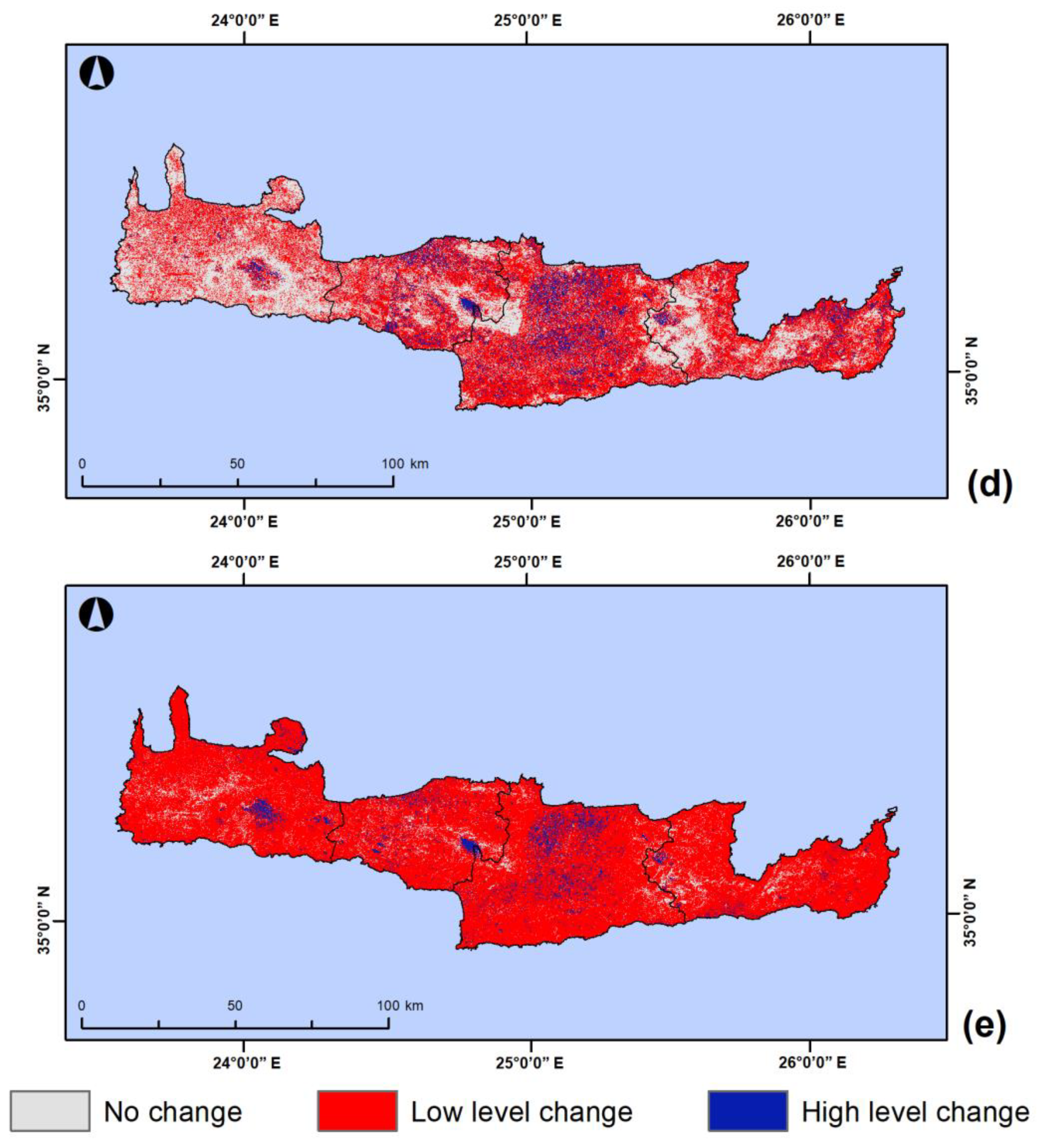
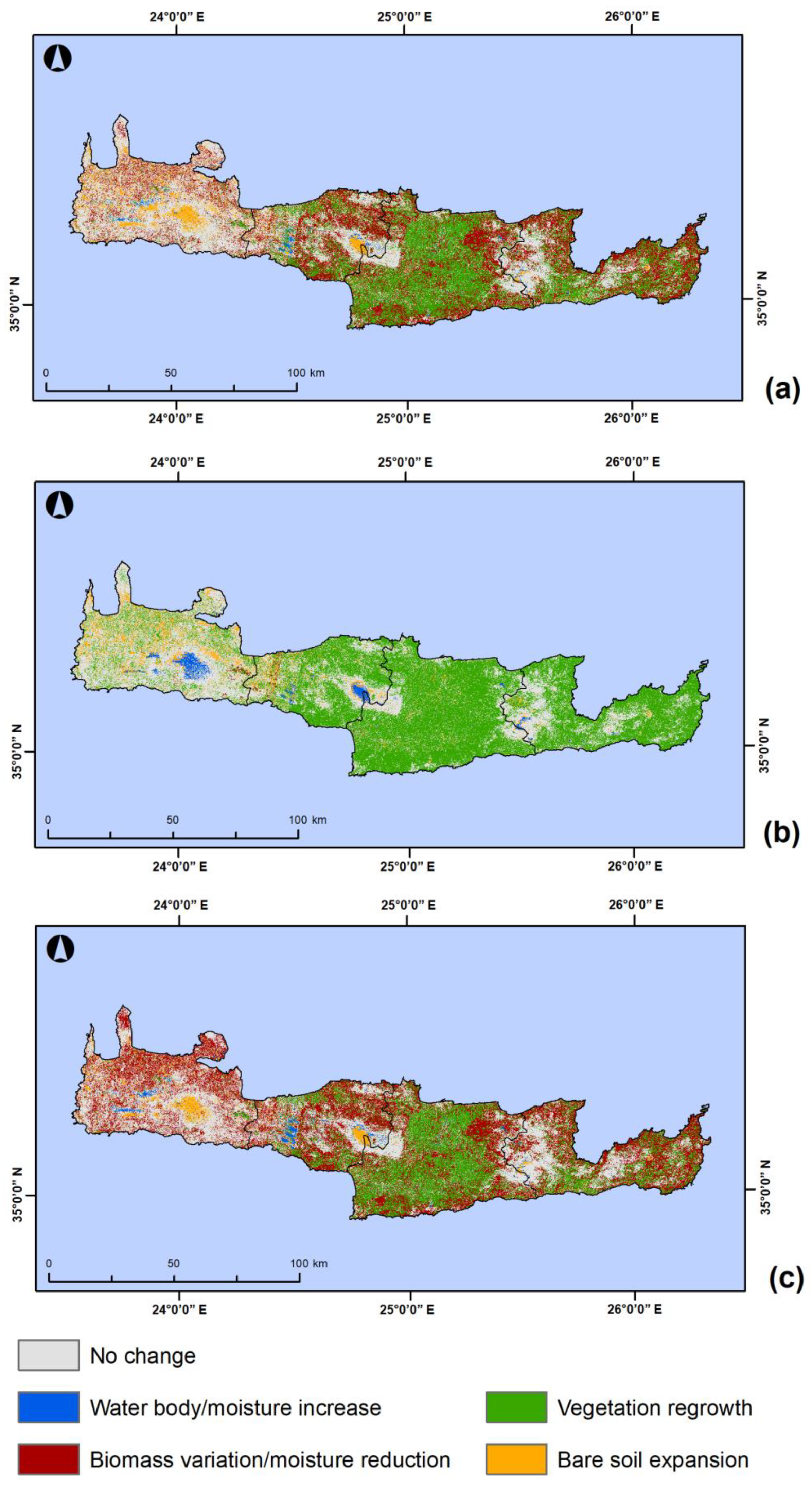
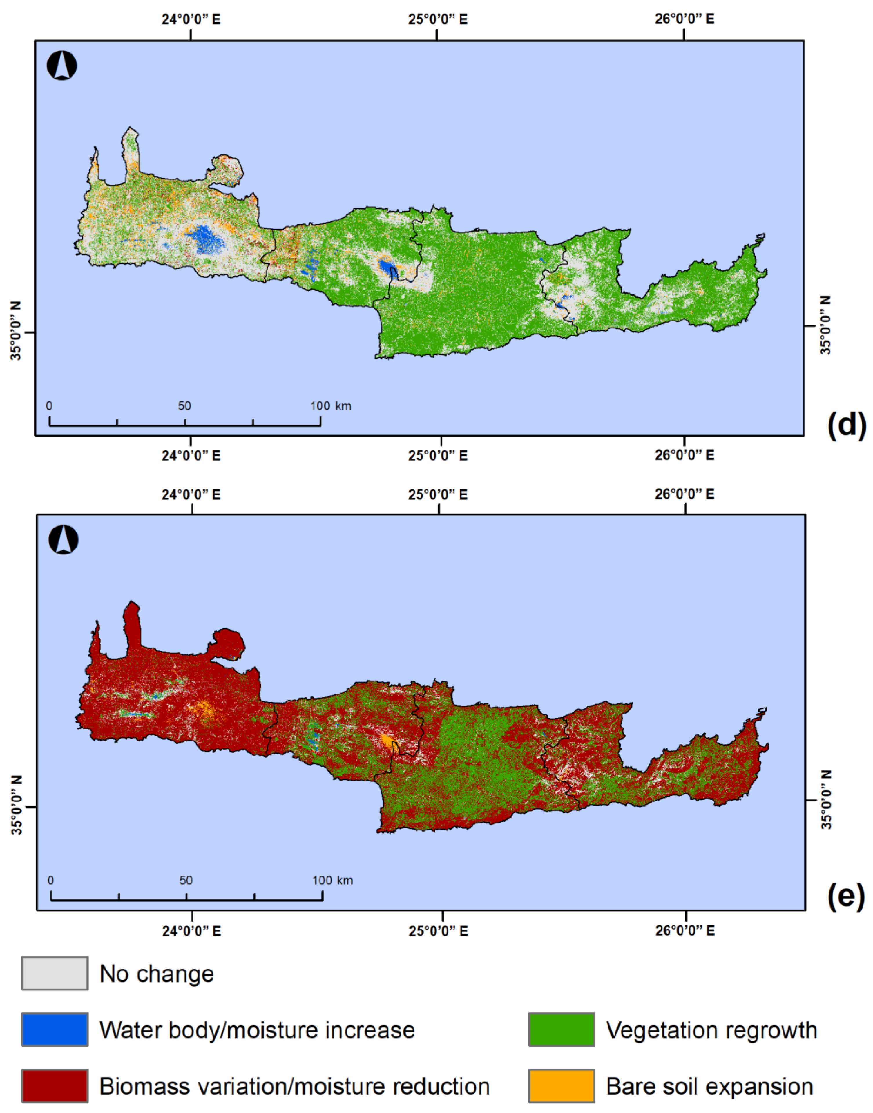
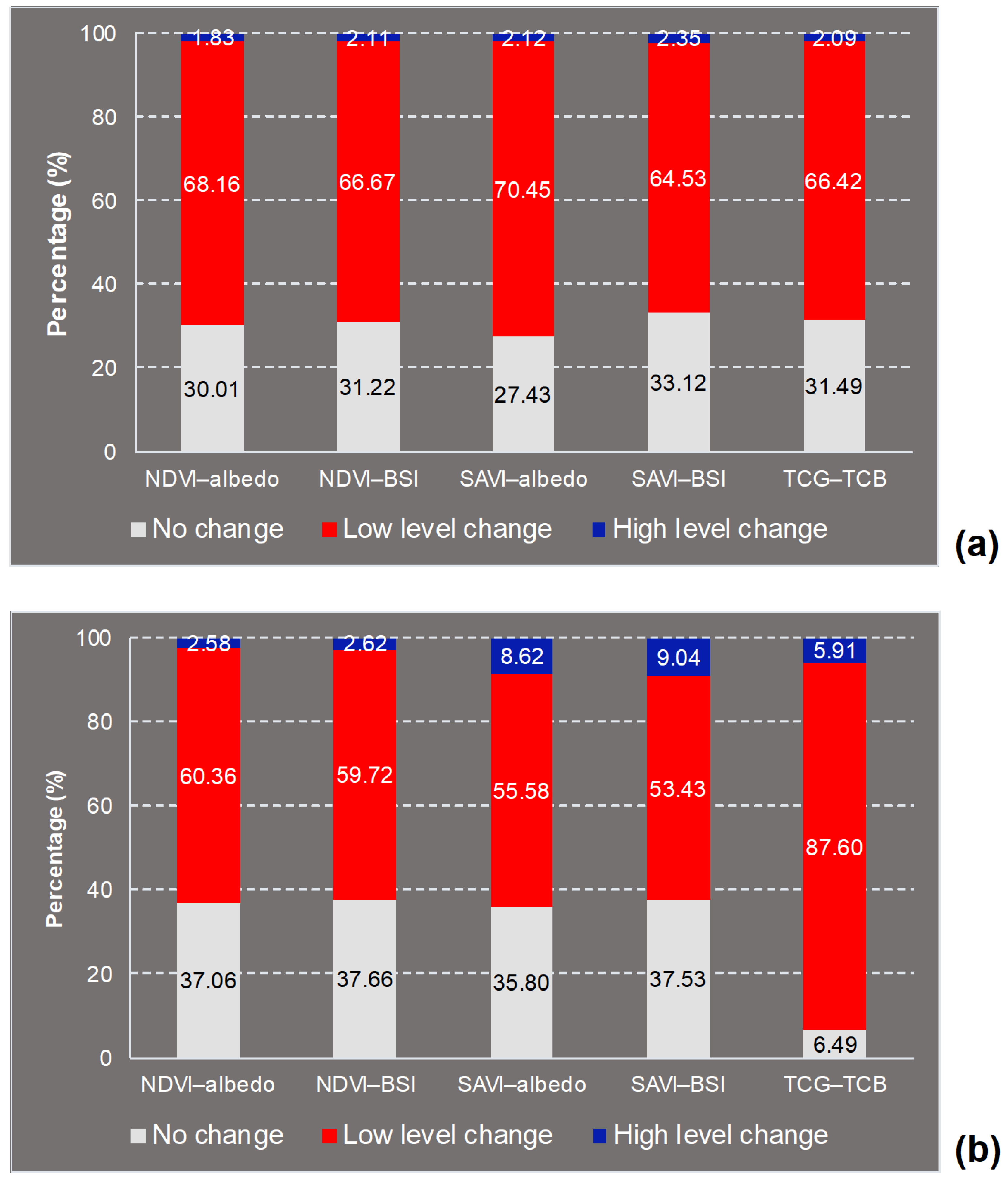
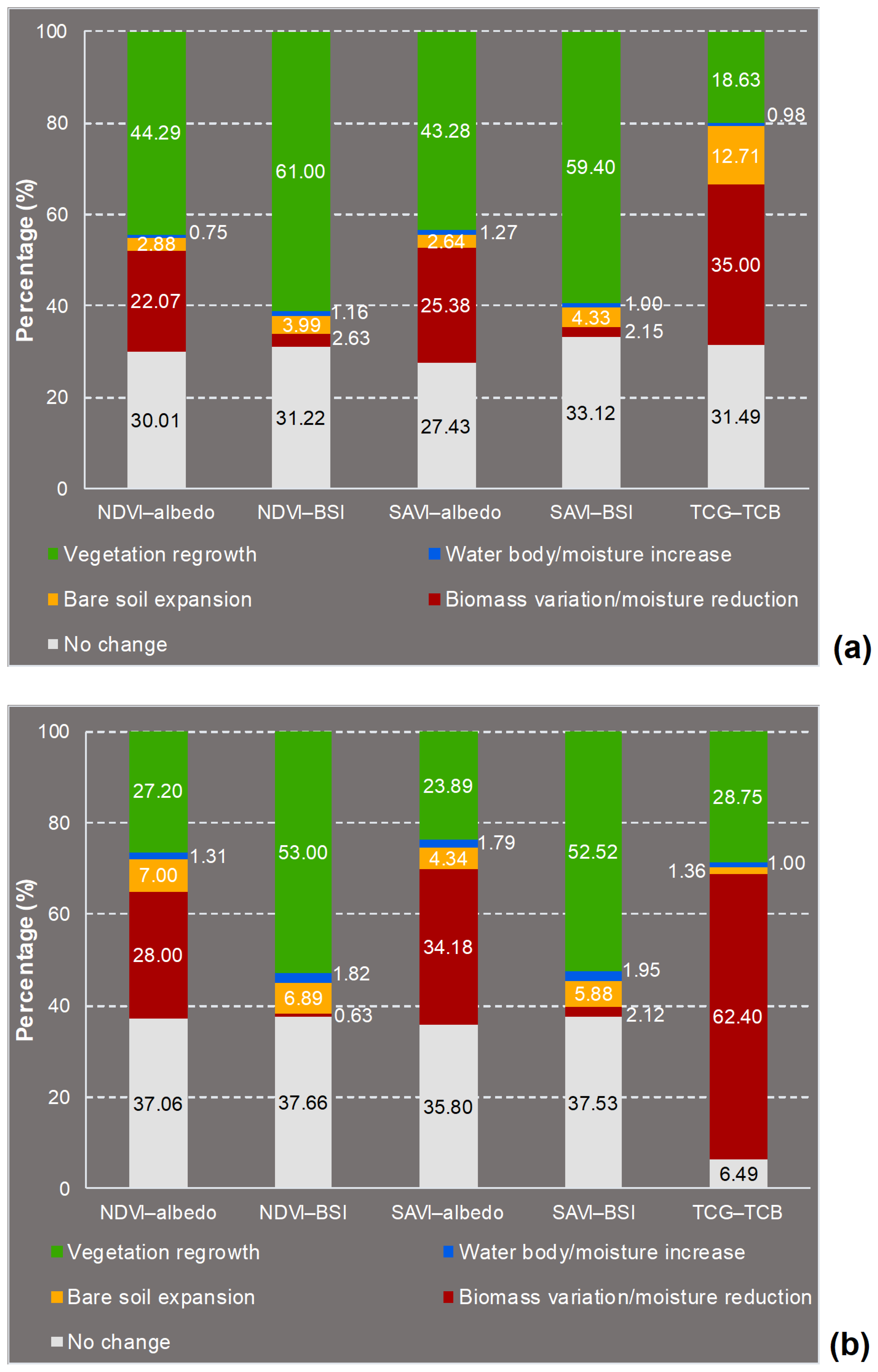
3.1. Spatio-Temporal Dynamics of Land Cover

The land cover change maps produced by the five examined index combinations in CVA are illustrated in Figure 4 and Figure 5 for the period of 1999–2009, and in Figure 6 and Figure 7 for the period of 2009–2019. Furthermore, the calculated area percentages of the relative categories are shown in Figure 8 and Figure 9, analytically, for each combination.

3.1.1. NDVI–Albedo

Based on the NDVI–albedo combination, a total of 69.99% (about 5779 km²) of the study area presented changes in the period between 1999 and 2009, with the rest, 30.01% (approximately 2478 km²), not presenting changes. Among the changes, 68.16% (about 5626 km²) of the island referred to low level changes detected across its total extent. Only 1.83% (about 153 km²) referred to high level changes mainly concentrated in the Rethymno prefecture.

In terms of change direction, i.e., type of change, 44.29% (approximately 3656 km²) of the study area indicated vegetation regrowth, followed by 22.07% (approximately 1822 km²), 2.88% (approximately 239 km²), and 0.75% (approximately 62 km²) indicating biomass variation/moisture reduction, bare soil expansion, and water body/moisture increase, respectively, in the same period. In either high or low degree, these change direction categories made their appearance across the entire region.

In the period between 2009 and 2019, a larger part of the study area (37.06%, approximately 3060 km²) remained unchanged thus resulting in a smaller changed part (total of 62.94%, approximately 5197 km²). Although the low-level changes continued to dominate on the island against the high level changes, a decrease in the first one (new percentage equal to 60.36%, approximately 4983 km²) and a slight increase in the second one (new percentage equal to 2.58%, approximately 214 km²) was noted. Spatially, the extent of the low-level changes decreased in the Chania prefecture, whereas the high-level changes were mostly concentrated in the Heraklion prefecture. However, a significant area of these changes remained in the Rethymno prefecture and especially on Psiloritis Mount.

In the same period, the part of the study area presenting vegetation regrowth was notably decreased (new percentage equal to 27.20%, approximately 2246 km²) reaching the extent of the part with biomass variation/moisture reduction (new percentage equal to 27.43%, approximately 2311 km²). This change type was limited in the Heraklion prefecture. On the other hand, the part presenting bare soil expansion increased (new percentage equal to 7%, approximately 532 km²) covering scattered areas in the Chania prefecture and large areas on the massifs of the island.

3.1.2. NDVI–BSI

According to the NDVI–BSI combination, a total of 68.78% (approximately 5680 km²) of the study area was observed with changes in the period between 1999 and 2009, and the rest 31.22% (approximately 2577 km²) with no changes. From the total of changed area, 66.67% (approximately 5504 km²) was related to low level changes, and only 2.11% (approximately 176 km²) to high level changes. The spatial pattern followed by these changes was shown to be similar to this one from NDVI–albedo combination in the same period.

As it was derived from the relative change direction map for the period of 1999–2009, 61% (approximately 5096 km²) of the island affected by vegetation regrowth, with only 3.99% (approximately 330 km²), 2.63% (approximately 218 km²), and 1.16% (approximately 36 km²) affected by bare soil expansion, biomass variation/moisture reduction, and water body/moisture increase, respectively. Areas with vegetation regrowth were detected across the entire island, and areas with bare soil expansion were mainly located in Heraklion prefecture. A high-level change to barren land was also extensively situated in the western part of the Lasithi prefecture and specifically on the Dikti Mount.

In the period between 2009 and 2019, the unchanged areas cover a larger part of the island (37.66%, approximately 3110 km²) resulting, thus, to a totally smaller part for changed areas (62.93%, approximately 5148 km²). Concerning the level of change, a decrease in the low-level changes (new percentage equal to 59.72%, approximately 4931 km²) and a slight increase in the high-level changes (new percentage equal to 2.62%, approximately 217 km²) were shown. Spatially, the withdrawal of the low-level changes from the western part of the island and the transfer of concentration of the high-level changes in the Heraklion prefecture and on Psiloritis Mount were also observed in this index combination.

The part of the study area indicating vegetation regrowth decreased (new percentage equal to 53%, approximately 4376 km²) and the part indicating bare soil expansion was slightly increased (new percentage equal to 7%, approximately 569 km²) in the period of 2009–2019. However, the large areas on Lefka Ori Mount (in Chania prefecture) and Psiloritis Mount (in Rethymno prefecture) affected by water body/moisture increase changes were the most pronounced from this index combination for the given period. A slight increase of the area percentage (new equal to 1.31% approximately 151 km²) was estimated for the relative change direction category.

3.1.3. SAVI–Albedo

The change magnitude map of SAVI–albedo combination for the period between 1999 and 2009 indicated that in total 72.57% (about 5993 km²) of the study area was changed, and the rest 27.43% (about 2264 km²) was unchanged. In particular, 70.45% (approximately 5816 km²) of the changes were of low level presenting a scattered distribution within the island. Only 2.12% (approximately 177 km²) of the changes were of high level, being mainly concentrated in the Rethymno prefecture.

The change direction map for the same period showed that a significant part equal to 43.28% (approximately 5096 km²) of the study area experienced vegetation regrowth. A less extensive part equal to 25.38% (approximately 2096 km²) experienced biomass variation/moisture reduction. Large extents of the aforementioned parts were detected in Rethymno prefecture. The corresponding area percentages for the other two categories, the bare soil expansion and water body/moisture increase, were 2.64% (approximately 219 km²) and 1.27% (about 105 km²), respectively.

In the period between 2009 and 2019, the total of unchanged areas increased (new percentage equal to 35.80%, approximately 2956 km²) and this area’s changed decreased (new percentage equal to 64.20%, approximately 5302 km²). However, despite the minimization of total changed extent, the areas with high level changes marked a notable increase reaching an area percentage equal to 8.62% (approximately 713 km²). These areas were situated across the entire island, with pronounced concentrations in its central part and specifically in the Heraklion and Rethymno prefectures. It is also worth mentioning the significant presence of this change magnitude category on Psiloritis Mount.

In the period of 2009–2019, the part of the study area experienced vegetation regrowth remarkably decreased (new percentage equal to 23.89%, approximately 1972 km²). This part was spatially restricted within Heraklion prefecture. On the contrary, the extent of the other three change direction categories more (new percentage equal to 34.18% or approximately 2824 km² for the biomass variation/moisture decrease) or less increased (new percentage equal to 4.34% or approximately 358 km² for the bare soil expansion, and to 1.79% or approximately 148 km² for the water body/moisture decrease). In the relative map, large areas seemed to experience bare soil expansion on Lefka Ori and Psiloritis Mounts and moisture increase in Chania and Rethymno prefectures.

3.1.4. SAVI–BSI

The change magnitudes from SAVI–BSI combination for the period of 1999–2009 can be characterized as quantitatively and spatially similar to the previous combinations. Changes occurred in the largest part of the study area (totally 66.88%, approximately 5523 km²). Most of these changes were of low level, covering 64.53% (approximately 5327 km²) of the island and presenting a spatial scattering across its total extent. The rest 2.35% (approximately 196 km²) was covered by high level changes which mostly took place in the Rethymno prefecture.

Based on change directions for the same period, vegetation regrowth occurred in the largest part of the study area (59.40%, approximately 5096 km²) indicating a spatially scattered coverage. Its relative percentage was found to be not at all close with those of the remaining categories which had a range from only 1% (approximately 41 km²) for water body/moisture reduction to 4.33% (approximately 359 km²) for bare soil expansion. However, the high spatial concentration of bare soil expansion in Heraklion prefecture must be highlighted.

As in the previously described combination of SAVI–albedo, so in this one, the increase to the extent of high-level changes (new percentage equal to 9.04%, approximately 747 km²) in the period of 2009–2019 was noticeable. Spatially, this increase was extended in significant parts of the Heraklion and Rethymno (remarkably on Psiloritis Mount) prefectures.

In the period of 2009–2019, vegetation regrowth occurred in a slightly smaller part of the island (52.52%, approximately 4335 km²). On the other hand, firstly bare soil expansion and subsequently moisture increase occurred in larger parts (5.88% or approximately 486 km², and 1.95% or approximately 162 km², respectively). Bare soil expansion was spatially transferred from the Heraklion to Chania prefecture, and the moisture increase replaced the relative areas of bare soil expansion on Lefka Ori and Psiloritis Mounts, as they were characterized by the previous SAVI–albedo combination.

3.1.5. TCG–TCB

Regarding the TCG–TCB combination results for the period between 1999 and 2009, a significant part of the study area totaling to 68.91% (approximately 5690 km²) indicated changes, with 66.42% (approximately 5484 km²) being linked to a low level and the rest 2.09% (approximately 173 km²) to a high level. A smaller part equal to 31.49% (approximately 2597 km²) indicated persistence. Persistent and low-level changed areas appear across the entire island, whereas high level changed areas mainly in the Heraklion prefecture.

Against all the above index combinations, this one indicated biomass variation/moisture reduction (not vegetation regrowth) as the change direction category with the highest coverage (36.19%, approximately 3021 km²) for the period of 1999–2009. A high concentration of this category in the southern part of Chania prefecture can be spatially detected. In a ranking based on area percentages, the categories of vegetation regrowth (18.63%, approximately 1539 km²), bare soil expansion (12.71%, approximately 1050 km²) and water body/moisture increase (0.98%, approximately 81 km²) follow. Areas with vegetation regrowth made their appearance in all prefectures of the island, whereas areas with bare soil expansion were highly concentrated in Heraklion prefecture.

In the period between 2009 and 2019, the extent of low-level changes increased covering an extremely large part of the study area (87.60%, approximately 7234 km²). A much smaller part (5.91%, about 488 km²) covered by a slightly increased extent of high-level changes was also observed in Heraklion prefecture, with large areas on Lefka Ori and Psiloritis Mounts.

In the period of 2009–2019, the part of the island indicating biomass variation/moisture reduction was almost doubled (new percentage equal to 62.40%, approximately 5205 km²). This doubling was followed by a lower increase in vegetation regrowth (new percentage equal to 28.75%, approximately 2374 km²), a significant decrease in bare soil expansion (new percentage equal to 1.36%, approximately 112 km²), and a persistence in water body/moisture increase (new percentage equal to 1%, approximately 31 km²). The high concentrations of areas with biomass variation/moisture reduction and vegetation regrowth in Heraklion and Chania prefectures, respectively, as well as the significant extent of areas with bare soil expansion on Psiloritis and Lefka Ori Mounts, constituted the most pronounced spatial characteristics from this index combination.

3.2. Accuracy Assessment

The outputs of CVA were evaluated by confusion matrices in terms of accuracy [33,34]. A confusion matrix provides accuracy statistics such as kappa index (with a range from 0 to 1 indicating from very low to excellent accuracy) and overall accuracy, according to the proportion of an area that is correctly matched with reference data [35]. Due to the unavailability of accurate field-derived data, new remote sensing-derived data was created to be used as reference data. Its creation was based on detailed land cover maps produced by supervised classification of the Landsat imagery data.

Analytically, a total of 246 random sample areas were firstly collected on RGB color composite images of 1999, 2009, and 2019. These areas were then labeled as a specific land cover category by visual interpretation resulting to the representation of totally six categories. Using the labeled areas, a supervised classification algorithm like Mahalanobis distance was applied in ENVI software to produce a detailed land cover map for each date (Figure 10). Based on the correlations within a dataset as well as the distribution of the data, Mahalanobis distance algorithm determines the similarity between an unknown data element to a known dataset by using a covariance matrix [36]. Consequently, a GIS-based spatial analysis was conducted on pairs of these maps identifying areas of change or no change for the periods 1999–2009 and 2009–2019. In changed area, the type of change was also identified and labeled according to the change direction categories from CVA. The total of identified information as reference data was finally compared with the change magnitude and direction outputs of CVA in confusion matrices to calculate the statistics of kappa index and overall accuracy (

Table 2. Kappa index and overall accuracy values calculated for different index combinations in two time periods.

Time Period	Index Combination	Change/No Change (Magnitude)		Type of Change (Direction)
		Kappa Index	Overall Accuracy	Kappa Index	Overall Accuracy
1999–2009	NDVI–albedo	0.672 1	0.954	0.637	0.887
	NDVI–BSI	0.669	0.949	0.590	0.862
	SAVI–albedo	0.664	0.943	0.626	0.884
	SAVI–BSI	0.668	0.949	0.591	0.863
	TCG–TCB	0.663	0.943	0.590	0.861
2009–2019	NDVI–albedo	0.686	0.960	0.637	0.896
	NDVI–BSI	0.676	0.954	0.612	0.883
	SAVI–albedo	0.673	0.946	0.631	0.889
	SAVI–BSI	0.675	0.950	0.616	0.884
	TCG–TCB	0.641	0.938	0.605	0.880

¹ Bold style indicates the highest values.

).

On the basis of areas with change and no change, for the period of 1999–2009, the highest values of kappa index and overall accuracy were derived from the NDVI–albedo combination. It was followed by NDVI–BSI, SAVI–BSI, SAVI–albedo, and TCG–TCB. For the period of 2009–2019, the highest values were also from NDVI–albedo followed by the same combinations.

Moreover, in terms of the type of change, for the period of 1999–2009, the highest values of kappa index and overall accuracy were from the NDVI–albedo. The SAVI–albedo, SAVI–BSI, NDVI–BSI and TCG–TCB constituted the ranking of the other combinations. For the period of 2009–2019, the ranking of the combinations was found to be similar.

4. Discussion and Interpretation

In the last two decades, the main objective of research efforts related to land cover change detection has been to produce reliable cartographic outputs with as high as possible accuracy. In this study, by applying a remote sensing-based technique like CVA, the relationship between the changes on various spectral indices and land cover changes in Crete Island was assessed and mapped for the time periods of 1999–2009 and 2009–2019. Landsat satellite images acquired in 1999, 2009 and 2019 constituted the basis for the creation of both vegetation and soil indices. Five different combinations of these indices (NDVI–albedo, NDVI–BSI, SAVI–albedo, SAVI–BSI and TCG–TCB) were examined in CVA in order to evaluate their impact on the performance of technique and identify the best combination in terms of accuracy of the outputs.

Change vector analysis is a robust change detection technique which can provide rich quantitative and qualitative information with respect to spatio-temporal land cover dynamics in a given region. Due to the fact of its two output products, change magnitude and direction, it enables the identification of different magnitudes and types of change. In comparison with classification-based techniques, CVA has the capability to concurrently analyze a set of remotely sensed data for monitoring changes within land cover classes. These changes are derived from the difference between successive satellite images without the need to struggle with uncertain classification [21].

The outputs of CVA for the different index combinations were mapped in order to visualize the spatial distribution of the estimated land cover change magnitudes and directions (i.e., types) in the study area. The magnitude maps (Figure 4 and Figure 5) produced by the total of combinations indicated that for both examined time periods the study area was mostly affected by low level changes. On the other hand, its unchanged part was also prominent. The presence of high-level changes was particularly low during the period of 1999–2009 presenting a similar spatial pattern across the island for the majority of combinations (except for TCG–TCB). However, this presence increased (specifically from SAVI–albedo and SAVI–BSI combinations) during the period of 1999–2009 covering much more areas in Heraklion and Rethymno prefectures as well as large areas on massifs of the island.

The direction maps (Figure 6 and Figure 7) created from the majority of combinations (except for TCG–TCB) indicated that during the period of 1999–2009 the study area mostly experienced land improvement expressed by vegetation regrowth. Due to the spatial concentration of this regrowth mainly in the western (Chania prefecture) and central (Rethymno prefecture) parts of the island, the high annual precipitation of the period [37] with the relative increasing amount of rainfall water from east to west (as a result of its spatial variability) can be characterized as the main natural driving force. On the other hand, the intensification of the agricultural sector had also an anthropogenic influence on the dominant type of land cover change. This intensification reached a high point in the specific period with complete mechanization of land cultivation and expansion of irrigation networks [38].

Based on the same index combinations, during the following period of 2009–2019, the study area continued to experience vegetation regrowth but to a decreased degree. Its spatial concentration was totally removed from the western to central part of the island (from Chania to Heraklion prefecture) leading to an increased land degradation in the west with more areas experiencing bare soil expansion. This higher spatial expansion of barren land can partially be attributed to the decrease in annual precipitation, which is projected to be further reduced over the next decades [39]. The precipitation decreases in this period altered the groundwater recharge with adverse implications for water supply and agricultural activities. In combination with that, the profit-based unattractiveness of traditional crops and the tourism growth caused further decline in the importance of the agricultural sector [38]. The bare soil expansion in large areas of massifs, such as Lefka Ori and Psiloritis Mounts, was also pronounced for the same period. The specific type of change, as it was noticed by the combinations of NDVI–albedo and SAVI–albedo, can be considered the result of accelerated rates of soil erosion in these mountainous areas.

In addition, it can be noted that a significant part of the previously described gain and loss of vegetation amount for the relative time periods was marked as less intense and was mostly “translated” as biomass variations (or moisture reduction) from the combination of TCG–TCB. This trend also appeared from the combinations of NDVI–albedo and SAVI–albedo in order to indicate much of vegetation loss within the period 2009–2019.

The part of the study area covered by water bodies or experiencing an increase in moisture is also worth mentioning. For this type of change, the small extent in both periods and the almost unchanged state between them, from the total of examined index combinations, constitute the confirmation of the limited presence of surface waters in the island.

Regarding the spectral indices used in the selected combinations it was shown that among the vegetation indices, SAVI had a different influence on change magnitude outputs providing more areas with high level changes against NDVI and TCG. In terms of change direction outputs, as it is derived from the above, among the soil indices, BSI seemed to highlight vegetation regrowth against biomass variations. Conversely, albedo and TCB highlighted the moisture of vegetation indicating these variations. Furthermore, in contrast to albedo and TCB, BSI was found to be greatly affected by the increased moisture of soil on massifs of the island (probably due to snow melting). The assignment of extensive mountainous areas (especially in the period of 2009–2019) to the relative category for the combinations with BSI, and to the category of bare soil expansion for the combinations with albedo and TCB confirms this finding.

Despite the differences among the examined indices, the magnitude and direction results produced by their combinations identified certain similarities. One of the most characteristic was the detection of land cover changes attributable to the construction of Aposelemis dam in Heraklion prefecture (Figure 1). In terms of magnitude, the total of the applied index combinations recognized the relative changes as high-level changes in both time periods. Moreover, in terms of direction, they firstly detected the beginning of the construction works in 2005 and the conversion of land from agricultural to barren (Figure 11), indicating the specific change as bare soil expansion for the period of 1999–2009. Afterwards, they detected the completion of the works in 2015 resulting to the creation of an artificial lake (Figure 11). In all the combinations, this change was represented by the category of water body/moisture increase for the period of 2009–2019.

The CVA outputs were evaluated in terms of accuracy using confusion matrices based on change/no change (magnitude) and change type (direction) for the two periods. The statistics of kappa index and overall accuracy calculated by these matrices (Table 2) showed that the five index combinations provided similar values of satisfactory accuracy. In general, among the pair of outputs, the combinations detected with higher accuracy the change/no change than the change type. Among the two periods, they detected with higher accuracy the changes that occurred in 2009–2019 than those in 1999–2009. However, for both kinds and for both periods, the combination of NDVI–albedo was found to have more accurate outputs than the other combinations. Thus, NDVI–albedo can be characterized as the most appropriate index combination for detecting the land cover changes in the study area. This finding is in agreement with the results from the research work of Vorovencii [33]. Specifically, by applying CVA for three different index combinations (NDVI–albedo, NDVI–brightness index and TCG–TCB), it was concluded that the most accurate outputs were obtained from the combination of NDVI–albedo.

The main limitations and assumptions of this work have to be pointed out. First of all, it is worth mentioning that CVA direction outputs provide dynamic and not static information about land cover changes. For example, the category representing vegetation regrowth neither indicates that the changed area was previously area with not at all vegetation, nor that it has changed to agricultural or forest area. Therefore, a good understanding of the change processes in the study area is required to improve on the interpretation of the direction outputs [40]. Furthermore, concerning the change magnitude outputs, the choice of thresholds for the determination between change and no change and between low- and high-level change, prove to be critical and play a major role in the accuracy of the relative outcomes. Since this choice was based on subjective criteria for the present study, the examination of alternative choices could lead to different results.

5. Conclusions

The changes of land cover occurred in a region may have serious environmental and socio-economic impacts. Therefore, the need for detecting these changes is more and more imperative, especially given the emergence of unbalances caused by natural and anthropogenic driving forces like climate change, intensive agriculture and wrong land management decisions. Considering this as well as the fact that the use of different remotely sensed data products is expected to have influence on the performance of a metric difference-based change detection technique, spatio-temporal land cover dynamics in the Greek island of Crete were detected and mapped for five different combinations of spectral indices using change vector analysis. The findings revealed that the selected technique, and thus land cover change detection, can be affected by the “nature” of indices. Furthermore, the promising evaluation results (with a range of 0.60–0.69 for kappa index and 0.86–0.96 for overall accuracy) of index combinations indicated that an accurate detection can be achievable. In particular, the confirmed, with higher accuracy (with a range of 0.64–0.69 for kappa index and 0.89–0.96 for overall accuracy), change magnitude and direction maps produced by the combination of NDVI–albedo could constitute an essential base for planners and decision-makers in identifying land cover changes and planning appropriate land management strategies. Due to the importance of agricultural land, which predominates in the island, it is extremely valuable the planning and implementation of such strategies in order to diminish the expansion of land degradation risk.

Future work could focus on the application of change vector analysis for detecting land cover changes in smaller regions contained in the island (e.g., watersheds) using satellite imagery of higher spatial resolution. Then, an identification of differences and similarities between the results of the two analysis scales (for the entire island and for the contained watersheds) could be achieved. Moreover, the comparison of change vector analysis with other change detection techniques, such as image differencing and principal component analysis, could be another objective of future work.

References

1. Moser, S.C. A partial instructional module on global and regional land use/cover change: Assessing the data and searching for general relationships. GeoJournal 1996, 39, 241–283. [Google Scholar] [CrossRef]
2. Ansari, A.; Golabi, M.H. Prediction of spatial land use changes based on LCM in a GIS environment for Desert Wetlands—A case study: Meighan Wetland, Iran. Int. Soil Water Conserv. Res. 2019, 7, 64–70. [Google Scholar] [CrossRef]
3. Alexakis, D.D.; Grillakis, M.G.; Koutroulis, A.G.; Agapiou, A.; Themistocleous, K.; Tsanis, I.K.; Michaelides, S.; Pashiardis, S.; Demetriou, C.; Aristeidou, K.; et al. GIS and remote sensing techniques for the assessment of land usechange impact on flood hydrology: The case study of Yialias basin in Cyprus. Nat. Hazards Earth Syst. Sci. 2014, 14, 413–426. [Google Scholar] [CrossRef] [Green Version]
4. Yirsaw, E.; Wu, W.; Shi, X.; Temesgen, H.; Bekele, B. Land Use/Land Cover Change Modeling and the Prediction of Subsequent Changes in Ecosystem Service Values in a Coastal Area of China, the Su-Xi-Chang Region. Sustainability 2017, 9, 1204. [Google Scholar] [CrossRef] [Green Version]
5. Patel, S.K.; Verma, P.; Shankar Singh, G. Agricultural growth and land use land cover change in peri-urban India. Environ. Monit. Assess. 2019, 191, 600. [Google Scholar] [CrossRef]
6. Singh, A. Digital change detection techniques using remotely-sensed data. Int. J. Remote Sens. 1989, 10, 989–1003. [Google Scholar] [CrossRef] [Green Version]
7. Islam, K.; Jasimuddin, M.; Nath, B.; Nath, T.K. Quantitative Assessment of Land Cover Change Using Landsat Time Series Data: Case of Chunati Wildlife Sanctuary (CWS), Bangladesh. Int. J. Environ. Geoinform. 2016, 3, 45–55. [Google Scholar] [CrossRef] [Green Version]
8. Liu, B.; Chen, J.; Chen, J.; Zhang, W. Land Cover Change Detection Using Multiple Shape Parameters of Spectral and NDVI Curves. Remote Sens. 2018, 10, 1251. [Google Scholar] [CrossRef] [Green Version]
9. Münch, Z.; Gibson, L.; Palmer, A. Monitoring Effects of Land Cover Change on Biophysical Drivers in Rangelands Using Albedo. Land 2019, 8, 33. [Google Scholar] [CrossRef] [Green Version]
10. Dawson, R.A.; Petropoulos, G.P.; Toulios, L.; Srivastava, P.K. Mapping and monitoring of the land use/cover changes in the wider area of Itanos, Crete, using very high resolution EO imagery with specific interest in archaeological sites. In Environment, Development and Sustainability; Springer: Dordrecht, The Netherlands, 2019; pp. 1–28. [Google Scholar]
11. Xystrakis, F.; Psarras, T.; Koutsias, N. A process-based land use/land cover change assessment on a mountainous area of Greece during 1945–2009: Signs of socio-economic drivers. Sci. Total Environ. 2017, 587–588, 360–370. [Google Scholar] [CrossRef] [PubMed]
12. Symeonakis, E. Modelling land cover change in a Mediterranean environment using Random Forests and a multi-layer neural network model. In Proceedings of the IEEE International Geoscience and Remote Sensing Symposium (IGARSS), Beijing, China, 10–15 July 2016. [Google Scholar]
13. Kolios, S.; Stylios, C.D. Identification of land cover/land use changes in the greater area of the Preveza peninsula in Greece using Landsat satellite data. Appl. Geogr. 2013, 40, 150–160. [Google Scholar] [CrossRef]
14. Mallinis, G.; Emmanoloudis, D.; Giannakopoulos, V.; Maris, F.; Koutsias, N. Mapping and interpreting historical land cover/land use changes in a Natura 2000 site using earth observational data: The case of Nestos delta, Greece. Appl. Geogr. 2011, 31, 312–320. [Google Scholar] [CrossRef]
15. Hellenic Statistical Authority (ELSTAT). Population and Housing Census: Resident Population. Available online: https://www.statistics.gr/el/statistics/pop (accessed on 22 November 2019).
16. Nikolaou, T.G.; Christodoulakos, I.; Piperidis, P.G.; Angelakis, A.N. Evolution of Cretan Aqueducts and Their Potential for Hydroelectric Exploitation. Water 2017, 9, 31. [Google Scholar] [CrossRef] [Green Version]
17. Tapoglou, E.; Vozinaki, A.E.; Tsanis, I. Climate Change Impact on the Frequency of Hydrometeorological Extremes in the Island of Crete. Water 2019, 11, 587. [Google Scholar] [CrossRef] [Green Version]
18. Kalisperi, D.; Kouli, M.; Vallianatos, F.; Soupios, P.; Kershaw, S.; Lydakis-Simantiris, N. A Transient ElectroMagnetic (TEM) Method Survey in North-Central Coast of Crete, Greece: Evidence of Seawater Intrusion. Geosciences 2018, 8, 107. [Google Scholar] [CrossRef] [Green Version]
19. United States Geological Survey (USGS). Available online: https://earthexplorer.usgs.gov/ (accessed on 15 October 2019).
20. Fernandes, P.J.F.; Furtado, L.F.; Raphael, G. Change vector analysis to detect deforestation and land use/land cover change in Brazilian Amazon. Braz. Geogr. J. Geosci. Humanit. Res. Medium 2014, 5, 371–387. [Google Scholar]
21. Karnieli, A.; Qin, Z.; Wu, B.; Panov, N.; Yan, F. Spatio-Temporal Dynamics of Land-Use and Land-Cover in the Mu Us Sandy Land, China, Using the Change Vector Analysis Technique. Remote Sens. 2014, 6, 9316–9339. [Google Scholar] [CrossRef] [Green Version]
22. Sangpradid, S. Change Vector Analysis using Integrated Vegetation Indices for Land Cover Change Detection. Int. J. Geoinform. 2018, 14, 71–77. [Google Scholar]
23. Song, C.; Woodcock, C.E.; Seto, K.C.; Lenney, M.P.; Macomber, S.A. Classification and change detection using Landsat TM data: When and how to correct atmospheric effects? Remote Sens. Environ. 2001, 75, 230–244. [Google Scholar] [CrossRef]
24. Chander, G.; Markham, B.L.; Helder, D.L. Summary of Current Radiometric Calibration Coefficients for Landsat MSS, TM, ETM+, and EO-1 ALI Sensors. Remote Sens. Environ. 2009, 113, 893–903. [Google Scholar] [CrossRef]
25. Peduzzi, P. Landslides and vegetation cover in the 2005 North Pakistan earthquake: A GIS and statistical quantitative approach. Nat. Hazards Earth Syst. Sci. 2010, 10, 623–640. [Google Scholar] [CrossRef]
26. Mróz, M.; Sobieraj, A. Comparison of several vegetation indices calculated on the basis of a seasonal SPOT XS time series and their suitability for land cover and agricultural crop identification. Tech. Sci. 2004, 7, 39–66. [Google Scholar]
27. Li, H.; Xie, Y.; Yu, L.; Wang, L. A Study on the land cover classification of arid region based on Multi-temporal TM images. Procedia Environ. Sci. 2011, 10, 2406–2412. [Google Scholar] [CrossRef] [Green Version]
28. Shandas, V.; Makido, Y.; Ferwati, S. Regional Variations in Temperatures. In Urban Adaptation to Climate Change: The Role of Urban Form in Mediating Rising Temperatures; Shandas, V., Skelhorn, C., Ferwati, S., Eds.; Springer Nature Switzerland AG: Cham, Switzerland, 2020. [Google Scholar]
29. Crist, E.P.; Cicone, R.C. A physically-based transformation of thematic mapper data-the TM tasseled cap. IEEE Trans. Geosci. Remote Sens. 1984, 22, 256–263. [Google Scholar] [CrossRef]
30. Huang, C.; Wylie, B.; Yang, L.; Homer, C.; Zylstra, G. Derivation of a tasseled cap transformation based on Landsat 7 at-satellite reflectance. Int. J. Remote Sens. 2002, 23, 1741–1748. [Google Scholar] [CrossRef]
31. Baig, M.H.A.; Zhang, L.; Shuai, T.; Tong, Q. Derivation of a tasselled cap transformation based on Landsat 8 at-satellite reflectance. Remote Sens. Lett. 2014, 5, 423–431. [Google Scholar] [CrossRef]
32. Duy, N.B.; Giang, T.T.H.; Son, T.S. Study on vegetation indices selection and changing detection thresholds selection in Land cover change detection assessment using change vector analysis. In Proceedings of the 6th International Congress on Environmental Modelling and Software, Leipzig, Germany, 1–5 July 2012; p. 235. [Google Scholar]
33. Vorovencii, I. Applying the change vector analysis technique to assess the desertification risk in the south-west of Romania in the period 1984–2011. Environ. Monit. Assess. 2017, 189, 524. [Google Scholar] [CrossRef]
34. Rahman, S.; Mesev, V. Change Vector Analysis, Tasseled Cap, and NDVI-NDMI for Measuring Land Use/Cover Changes Caused by a Sudden Short-Term Severe Drought: 2011 Texas Event. Remote Sens. 2019, 11, 2217. [Google Scholar] [CrossRef] [Green Version]
35. Congalton, R.G.; Green, K. Assessing the Accuracy of Remotely Sensed Data: Principles and Practices, 2nd ed.; CRC Press: Boca Raton, FL, USA, 2009; p. 183. [Google Scholar]
36. Srivastava, N.; Rao, S. Learning-based text classifiers using the Mahalanobis distance for correlated datasets. Int. J. Big Data Intell. 2016, 3, 1–9. [Google Scholar] [CrossRef]
37. Agou, V.D.; Varouchakis, E.A.; Hristopulos, D.T. Geostatistical analysis of precipitation in the island of Crete (Greece) based on a sparse monitoring network. Environ. Monit. Assess. 2019, 191, 353. [Google Scholar] [CrossRef]
38. Detsis, V.; Briassoulis, H.; Kosmas, C. The Socio-Ecological Dynamics of Human Responses in a Land Degradation-Affected Region: The Messara Valley (Crete, Greece). Land 2017, 6, 45. [Google Scholar] [CrossRef] [Green Version]
39. Steiakakis, E.; Vavadakis, D.; Kritsotakis, M.; Voudouris, K.; Anagnostopoulou, C. Drought impacts on the fresh water potential of a karst aquifer in Crete, Greece. Environ. Earth Sci. 2016, 75, 507. [Google Scholar] [CrossRef]
40. Siwe, R.N.; Koch, B. Change vector analysis to categorise land cover change processes using the tasselled cap as biophysical indicator. Environ. Monit. Assess. 2008, 145, 227–235. [Google Scholar] [CrossRef]
Figure 1. Study area and location maps.
Remotesensing 12 00319 g001
Figure 2. The concept of change vector analysis for two-dimensional space: (a) change magnitude; (b) change direction.
Remotesensing 12 00319 g002
Figure 3. Spectral indices for selected dates: (a) normalized difference vegetation index (NDVI) for 1999; (b) soil adjusted vegetation index (SAVI) for 2009; (c) tasseled cap greenness (TCG) for 2019; (d) Albedo for 1999; (e) bare soil index (BSI) for 2009; (f) tasseled cap brightness (TCB) for 2019.
Remotesensing 12 00319 g003aRemotesensing 12 00319 g003b
Figure 4. Change magnitude maps for the period of 1999–2009 from different index combinations: (a) NDVI–albedo; (b) NDVI–BSI; (c) SAVI–albedo; (d) SAVI–BSI; (e) TCG–TCB.
Remotesensing 12 00319 g004aRemotesensing 12 00319 g004b
Figure 5. Change direction maps for the period of 1999–2009 from different index combinations: (a) NDVI–albedo; (b) NDVI–BSI; (c) SAVI–albedo; (d) SAVI–BSI; (e) TCG–TCB.
Remotesensing 12 00319 g005aRemotesensing 12 00319 g005b
Figure 6. Change magnitude maps for the period of 2009–2019 from different index combinations: (a) NDVI–albedo; (b) NDVI–BSI; (c) SAVI–albedo; (d) SAVI–BSI; (e) TCG–TCB.
Remotesensing 12 00319 g006aRemotesensing 12 00319 g006b
Figure 7. Change direction maps for the period of 2009–2019 from different index combinations: (a) NDVI–albedo; (b) NDVI–BSI; (c) SAVI–albedo; (d) SAVI–BSI; (e) TCG–TCB.
Remotesensing 12 00319 g007aRemotesensing 12 00319 g007b
Figure 8. Area percentages of change magnitude categories produced by different index combinations: (a) 1999–2009; (b) 2009–2019.
Remotesensing 12 00319 g008
Figure 9. Area percentages of change direction categories produced by different index combinations: (a) 1999–2009; (b) 2009–2019.
Remotesensing 12 00319 g009
Figure 10. Detailed land cover maps produced by supervised classification: (a) 1999, including the locations of 246 sample areas represented by point features; (b) 2009; (c) 2019.
Remotesensing 12 00319 g010
Figure 11. Multi-temporal Landsat color-infrared images focused on Aposelemis dam: (a) 1999; (b) 2009; (c) 2019.
Remotesensing 12 00319 g011