Article

Narrowband-to-Broadband Conversions for Top-of-Atmosphere Reflectance from the Advanced Very High Resolution Radiometer (AVHRR)

Royal Meteorological Institute of Belgium, B-1180 Brussels, Belgium
*
Author to whom correspondence should be addressed.
Remote Sens. 2020, 12(2), 305; https://doi.org/10.3390/rs12020305
Submission received: 20 December 2019 / Revised: 13 January 2020 / Accepted: 14 January 2020 / Published: 17 January 2020
(This article belongs to the Special Issue Earth Radiation Budget)

Abstract

:
The current lack of a long, 30+ year, global climate data record of reflected shortwave top-of-atmosphere (TOA) radiation could be tackled by relying on existing narrowband records from the Advanced Very High Resolution Radiometer (AVHRR) instruments, and transform these measurements into broadband quantities like provided by the Clouds and the Earth’s Radiant Energy System (CERES). This paper presents the methodology of an AVHRR-to-CERES narrowband-to-broadband conversion for shortwave TOA reflectance, including the ready-to-use results in the form of scene-type dependent regression coefficients, allowing a calculation of CERES-like shortwave broadband reflectance from AVHRR channels 1 and 2. The coefficients are obtained using empirical relations in a large data set of collocated, coangular and simultaneous AVHRR-CERES observations, requiring specific orbital conditions for the AVHRR- and CERES-carrying satellites, from which our data analysis uses all available data for an unprecedented observation matching between both instruments. The multivariate linear regressions were found to be robust and well-fitting, as demonstrated by the regression statistics on the calibration subset (80% of data): adjusted R 2 higher than 0.9 and relative RMS residual mostly below 3%, which is a significant improvement compared to previous regressions. Regression models are validated by applying them on a validation subset (20% of data), indicating a good performance overall, roughly similar to the calibration subset, and a negligible mean bias. A second validation approach uses an expanded data set with global coverage, allowing regional analyses. In the error analysis, instantaneous accuracy is quantified at regional scale between 1.8 Wm 2 and 2.3 Wm 2 (resp. clear-sky and overcast conditions) at 1 standard deviation (RMS bias). On daily and monthly time scales, these errors correspond to 0.7 and 0.9 Wm 2 , which is compliant with the GCOS requirement of 1 Wm 2 .

Graphical Abstract

1. Introduction

Broadband measurements of top-of-atmosphere (TOA) reflected solar flux and emitted thermal flux are essential climate variables of which a high-quality data record of satellite measurements with sufficient length (“Climate Data Record” or CDR) is needed by, among others, the climate modeling community (for validation purposes), and preferably spanning several decades [1]. However, apart from instrument-specific broadband measurement campaigns (e.g., CERES, 2000-present [2]) and regional datasets based on geostationary satellites (e.g., Meteosat-based, 1983–2015 [3]), to date no harmonized global CDR dating back several decades exists. An alternative method is to rely on existing global long-term CDRs of harmonized narrowband reflectance (FCDRs), e.g., from the Advanced Very High Resolution Radiometer (AVHRR) instrument [4,5], and transform these measurements into broadband quantities [6]. This study aims to establish robust relations between the long-term record of narrowband AVHRR measurements, and the relatively recent state-of-the-art broadband measurements from CERES: these results allow the generation of a global, long-term, broadband energy balance dataset, that would fit the needs of the climate modeling and monitoring community.
Narrowband-to-Broadband (NTB) corrections can be developed in two different ways [7]: (a) data sets with pairs of collocated, coangular and simultaneous narrowband (i.e., spectral) and broadband observations (also referred to as “matched NTB pairs”) can empirically be analyzed with regression methods, or (b) theoretical simulations of NTB corrections using sophisticated radiation models may be used [8,9]. Here we focus on the first, empirical method, for which there are basically three possibilities of obtaining matched NTB pairs:
A first possibility is that the narrowband and broadband instruments are located on the same satellite. In this case, all matched NTB pairs are per definition highly collocated, coangular, and simultaneous. Examples include CZCS and ERB on Nimbus-7 satellite [10], AVHRR and ERBE on NOAA-9 satellite [11,12], SEVIRI and GERB on Meteosat satellite [3]. While this is obviously the easiest way to obtain a large database of matched NTB pairs, the instrument combinations are limited.
A second possibility is to combine a broadband instrument located on a polar orbiting satellite (e.g., ERB, ERBE, CERES, ScaRaB) with a narrowband instrument located on a geostationary satellite (e.g., VISSR, SEVIRI). The geostationary satellite provides a fixed field of view with a relatively frequent temporal sampling. However, the coangularity criteria have as effect that the matching is restricted to certain regions, e.g., to the tropics when combining SEVIRI with cross-track CERES [13]. Examples include GOES2/VISSR to Nimbus7/ERB [14], Meteosat2/MVIRI to NOAA9/ERB [15], GOES7/VISSR to Meteor/ScaRaB [16], MSG1/SEVIRI to Terra-Aqua/CERES [13].
Finally, the narrowband and broadband sensors can be located on different polar orbiting satellites. This is rather challenging since both satellites are moving independently from each other and chances of simultaneous collocated and coangular measurements are rare, except if both orbital planes coincide and their speed (altitude) is significantly different to allow frequent catch-ups. Probably due to these specific requirements, this possibility is barely reported in the literature.
A brief overview of existing empirical NTB conversions for AVHRR is given in the review paper by Godøy and Eastwood [7]. The following studies are discussed, where AVHRR is used for planetary albedo determination: Wydick et al. [17] collocated AVHRR (NOAA-7) to ERB (Nimbus-7), but this study does not really belong to any of the mentioned methods since the narrowband (1981) and broadband (1978–1980) observations are not simultaneous. Li and Leighton [11] and Hucek and Jacobowitz [12] collocated AVHRR to ERBE, on the same satellite NOAA-9 (possibility 1).
This paper aims to improve on the last two mentioned studies by making new regressions between AVHRR and CERES, with the most notable advancement being the use of CERES Ed.4 broadband radiance products which, compared to ERBE, performs better due to several instrumental and processing improvements such as a higher resolution, better scene identification, more accurate auxiliary data (e.g., sea ice), etc. [18]. Furthermore, more detailed scene types are distinguished (e.g., “forest”, “grass”, or “savannas” instead of just “land”), for each of which a separate NTB regression is derived. Relating AVHRR narrowband to CERES broadband reflectance necessarily means a choice for the third empirical NTB possibility in the above mentioned framework.
Early studies proposed a linear regression that was solely dependent on the narrowband reflectances [11,12,14,17,19]. The equation used to relate narrowband reflectance (AVHRR channels 0.6 μ m and 0.8 μ m) to broadband reflectance ( ρ S W ) typically takes the following form:
ρ S W = b 0 + b 1 · ρ 0.6 + b 2 · ρ 0.8
where b x are the regression coefficients and ρ stands for “true isotropic reflectance” [4], also known as “Lambertian reflectance” [20], here simply referred to as reflectance. The values are expressed as percentage, with a range of 0–100. In subsequent studies, however, the regression parameters were found to depend moderately on solar zenith angle (SZA; θ 0 ) [21]. These studies therefore included θ 0 as additional parameter [16,22,23]. Feng and Leighton [23] furthermore found a dependency on viewing zenith angle (VZA; θ ). Built on this knowledge, the current study includes the SZA-dependency in the same way as Minnis et al. [22] and adds the VZA-dependency [23], resulting in the following regression equation:
ρ S W = b 0 + b 1 · ρ 0.6 + b 2 · ρ 0.8 + b 3 · l n 1 c o s ( θ 0 ) + b 4 · l n 1 c o s ( θ )
The inverse of the cosine being a good approximation for the atmospheric path. While the first two of above mentioned studies [16,22] removed anisotropy by applying a narrowband angular directional model (ADM), prior to the NTB conversion, the latter study [23] argued against this practice: it prevents the user from applying an ADM of his choice, e.g., anticipating on future improved ADMs. Their point of view is largely followed in this study, in which no a priori angular correction is applied. The resulting ρ S W can then be used in a broadband ADM of choice (e.g., [24,25,26], or anticipated future ADMs) to remove anisotropy and ultimately obtain the real hemispherical albedo and flux.

2. Data

The broadband measurements are taken from the instantaneous footprint data of the CERES instrument [27] onboard satellites Terra FM1 and Aqua FM3 (Single Scanner Footprint TOA/Surface Fluxes and Clouds edition 4A [28]). Apart from the actual broadband reflectance, also included are geophysical variables (e.g., cloud mask) simultaneously recorded by the accompanying MODIS imager and aggregated to CERES resolution. These will be compared to geophysical variables from AVHRR, to verify whether the matched NTB pair also has identical conditions (apart from the purely temporal-geometrical conditions). Footprint size and shape are spatially variable: cross-track and along-track dimensions increase with viewing zenith angle ( θ ) due to an increasingly spread-out projected area, which is even more magnified by the earth’s curvature. Assuming a spherical pixel with diameter of 32 km at nadir (PSF with 95% energy cutoff [29]), at θ = 70 its dimensions reach ~212 km (cross-track) and ~71 km (along-track).
The narrowband measurements are taken from the AVHRR instrument [30] onboard NOAA-17,-18,-19 satellites, from which an FCDR is created with Global Area Coverage Level-1c data created using the PyGAC processor [5]. This data set is supplemented with geophysical variables (such as cloud mask, sea ice concentration, etc.) remapped on the same grid [31]. The data have a spatial resolution of 4 km at nadir, but similar to CERES SSF, pixel size and shape are subject to biaxial deformation with increasing viewing zenith angle.
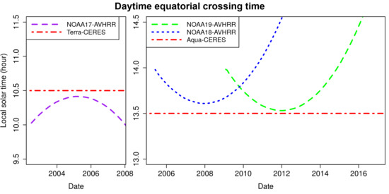
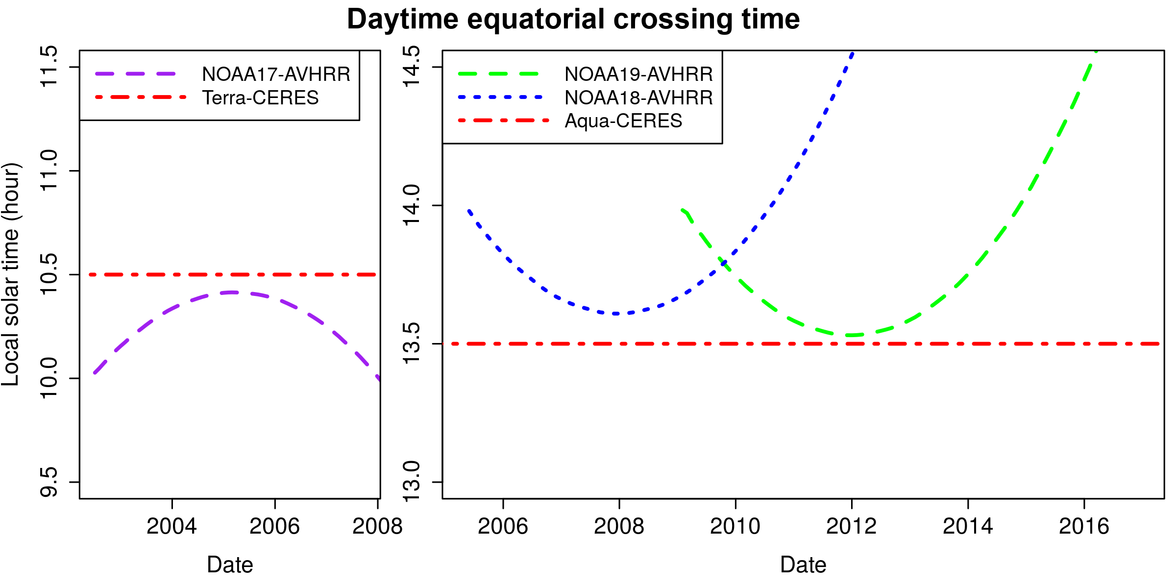
The analysis time period has been selected by examining the orbital planes of Terra/Aqua and NOAA satellites: the former have a true sun-synchronous orbit (with daytime equatorial crossing times of ~10:30 and ~13:30 LST) whereas the latter suffer from orbital drift (Figure 1). The orbital planes coincide around January 2005 (NOAA-17), 2008 (NOAA-18) and 2012 (NOAA-19), which then provides the necessary conditions for having frequent matched NTB pairs, i.e., simultaneous, collocated, and coangular. Since coinciding orbital planes of AVHRR- and CERES-carrying satellites did not occur outside these three time periods, this study analyses an unprecedented exhaustive amount of matched NTB pairs. Combining satellites with deviating orbital planes is not efficient, since there is only a marginal addition of NTB pairs at a high computational cost. This is illustrated by a small test on January 2012: the combination Aqua+NOAA19 (coinciding) results in 4.124.334 matched NTB pairs, whereas Aqua+NOAA18 (~1h off) generates only 99.605 pairs, or 2.4%, which furthermore occur in two limited high-latitude bands. To account for seasonal variability in spectral properties of some land cover types (such as vegetation or sea-ice), the full annual cycle is considered. Therefore, a range of at least +/−6 months is chosen around January, ending up with the periods given in Table 1. The long time span of a full year furthermore enables regressions per surface type, as the sample size must be large enough within each of these groups, and finally it also allows splitting off a smaller subset serving as independent observations for validation purposes.

3. Method

3.1. Data Preparation

An initial version of the dataset is constructed by identifying matched NTB pairs: based on temporal and spatial constraints, the algorithm iterates over all pixels in both datasets to find corresponding pixels.
In a first step, the CERES pixels are filtered on the criterion that it only contains either land, water, or snow (mixtures are excluded). Only water and sea ice are permitted to co-exist in a single CERES pixel. Then, the AVHRR pixel closest to the CERES pixel center is identified, but only considered if differences in 3D viewing angle (combining viewing zenith and azimuth) and observation time are less than 6 and 450 s [13], respectively. If so, based on the viewing geometry and assuming an at-nadir size of 32 × 32 km (cf. Appendix A.1), the footprint size of the CERES pixel is determined, the corresponding AVHRR pixels are identified (their centroids should be located inside the CERES footprint), and their associated radiance and other geophysical variables are aggregated. This converts the binary cloud mask, either 0 or 1, into a continuous cloud fraction between 0–100%. An additional constraint is that all AVHRR pixels should belong to the same surface type (first column in Table 2: ocean, forest, etc.), otherwise the pixel disqualifies and the iteration continues. Therefore the algorithm finds the nearest matching IGBP land cover category for each AVHRR pixel in a static 1 km grid IGBP map [32], followed by a mapping from IGBP category to surface type [33] as shown in the first two columns in Table 2. Sea ice surface types can only contain a mixture of ocean and sea ice, and are subdivided according to sea ice concentration: subdivisions are based on the non-linear relations between concentration, color and albedo due to the seasonal effects such as melting pond formation [34]. Finally, sun glint contamination is avoided by rejecting NTB pairs with a sun glint angle (between sun specular reflection and viewing direction) smaller than 25 [13]. The resulting dataset amounts over 45 million matched NTB pairs (Figure 2).
In a second step, filtering is performed on the resulting dataset. Matched NTB pairs are categorized according to their cloud fraction: “clear” and “overcast” pairs require both the CERES and AVHRR cloud fraction to exactly amount 0% and 100% respectively. “All-sky pairs” simply require that the difference between CERES and AVHRR cloud cover is no more than 20% point. At this point, the dataset contains over 35 million all-sky pairs and is referred to as the “expanded validation database” characterized by relaxed matching criteria (used in Section 3.3.2 and Section 4.3.2).
In a third step, the dataset is narrowed down to 3.3 million pairs by restricting angular and temporal matching criteria: for most NTB pairs, the maximum allowed temporal and 3D-angular differences between CERES and AVHRR observations are set to 250 s and 2.5 , respectively. These threshold values were established after an iterative trial-and-error process to find a trade-off between keeping a sufficiently large sample size (higher thresholds) and lowering angle/time difference error (lower thresholds). For surface types ocean and permanent snow, their areal abundance allows stricter criteria: 100 s and 1.0 respectively. For some scarce combinations of surface type and cloud cover (i.e., scene type), namely clear forests, overcast savannas and clear broken sea ice (60–10%), the thresholds are set to 300 s and 3.0 . Subsequently, for each scene type, every fifth pair in the chronologically ordered dataset is split off: these 20% of the pairs constitute the “smaller validation subset” characterized by strict matching criteria (used in Section 3.3.1 and Section 4.3.1). The remainder of the data constitutes the “calibration subset” (80% of the pairs), used to derive the NTB regression coefficients (about 2.7 million pairs).

3.2. Regression Calibration

For each scene type, a multivariate linear regression is performed on the calibration subset using the least squares method with AVHRR reflectance and solar/viewing zenith angles as predictors (Equation (2)). The resulting best-fit coefficients are stored together with the associated regression statistics (adjusted R 2 , absolute and relative RMS residual). Let ρ ^ S W and ρ S W be the estimated and observed broadband shortwave reflectance, then residual r i is defined as ( ρ ^ S W , i ρ S W , i ) and the sum of squared residuals (SSR) as ( i = 1 n r i 2 ), so that the surface-type-dependent Root-Mean-Square residual (RMSr) is calculated as follows:
R M S r = S S R n = 1 n · i = 1 n r i 2 = 1 n · i = 1 n [ ( ρ ^ S W , i ρ S W , i ) 2 ]
where n is the number of NTB pairs i within a given scene type. Please Note that the units of R M S r are identical to the units of reflectance, i.e., expressed as percentage and ranging from 0 to 100. The relative RMS residual (rRMSr) is defined as the absolute RMSr divided by the mean observed broadband shortwave reflectance ( < ρ S W > ), and can be expressed as fraction or percentage:
r R M S r = R M S r < ρ S W > = 1 n · i = 1 n [ ( ρ ^ S W , i ρ S W , i ) 2 ] 1 n · i = 1 n ρ S W , i
For each scene type, also two simpler regression models are constructed by using only 3 and 2 predictors, respectively (instead of 4 predictors in the complete model), from which the 2-predictor model is given by Equation (1). This allows to assessment of the added value of the additional predictors.
Finally, beside the surface-type-dependent regressions, a generic surface-type-independent regression is fitted by considering all matched NTB pairs regardless surface type. This regression allows to assessment of the added value of with a separate regression for each surface type.

3.3. Validation

3.3.1. Validation on Smaller Validation Subset (with Strict Matching Criteria)

To validate the surface-type-dependent NTB regression models obtained from the calibration subset, they are applied on narrowband AVHRR reflectance from the smaller validation subset (20% of the matched NTB pairs with strict matching criteria) using Equation (2). The resulting estimated broadband reflectance is compared with its observed equivalent (from CERES-SSF), and their difference quantified by the Mean Bias ( M B ) and relative Mean Bias ( r M B ) per scene type, each containing n NTB pairs:
M B = 1 n · i = 1 n ( ρ ^ S W , i ρ S W , i )
r M B = 1 n · i = 1 n ρ ^ S W , i ρ S W , i ρ S W , i
with ρ ^ S W the estimated and ρ S W the observed broadband reflectance. The statistical significance of M B is estimated by using Welch’s Two Sample t-test at 95% confidence level, meaning that when the p-value remains below 0.05 the null hypothesis is rejected and the means are considered significantly different. Furthermore, for each scene type, the reflectance bias is also expressed in terms of isotropic flux ( M B f l u x , Wm 2 ), also referred to as flux-equivalent Mean Bias, allowing a better assessment of the bias’ relevance since it is weighted by insolation:
M B f l u x = 1 n · i = 1 n [ ( ρ ^ S W , i ρ S W , i ) · 0.01 · T S I · c o s ( θ 0 , i ) ]
where T S I is the total solar irradiance (here taken at 1363 Wm 2 ). The statistical significance calculation of M B f l u x is equal to the one of M B .
This approach does not allow a regional (spatial) analysis since the strict matching criteria for both calibration and validation subsets limit the sampling, geographical coverage and hence the construction of global maps and globally aggregated metrics. This problem is tackled when using a different validation approach (Section 3.3.2).

3.3.2. Validation on Expanded Validation Database (with Relaxed Matching Criteria) and Regional Analysis

A second validation approach is to apply the surface-type-dependent NTB regressions on the narrowband reflectances from the expanded validation database, consisting of 35 million pairs with global coverage due to the relaxed matching criteria. The bias ( M B , r M B , M B f l u x ) between estimated and observed broadband reflectance is then calculated for each pair and stratified per surface type. Furthermore, to detect regional biases and to calculate a global mean bias regardless region-specific over- or undersampling of the matched NTB pairs, the expanded database is spatially aggregated into a 5 × 5 equirectangular grid. Prior to the global mean calculation, grid boxes with less than 32 observations are excluded and the grid is subjected to area-weighting [ c o s ( l a t i t u d e ) ]. Additional global statistics are calculated, such as the mean absolute bias (MAB) and RMS bias, both indicators for uncertainty at the 5 regional scale.

3.3.3. Added Value of Surface-Type-Dependent Regressions

Both above mentioned validations are also done using the generic surface-type-independent regression, which is applied on all NTB pairs regardless their surface type. The added value of having a separate NTB regression for each surface type is then assessed by comparing the validation results derived by surface-type-dependent and by surface-type-independent regression coefficients.

3.4. Error Budget

The error is separated in three components: the precision, the stability and the accuracy.

3.4.1. Precision

The precision refers to the non-systematic error associated with the derivation of the NTB regression. Note that this does not include the error associated with the input data (including the FCDR). The precision depends on the sample size, i.e., number of NTB pairs within each scene type (n) used to derive the NTB regressions, and is quantified by the standard error of residuals ( S E r ), calculated as the RMS residual divided by n :
S E r = R M S r n = 1 n · i = 1 n [ ( ρ ^ S W , i ρ S W , i ) 2 ]
Just like all other above mentioned metrics ( R a d j 2 , R M S r , r R M S r , M B , r M B , M B f l u x ), this quantity is calculated for each scene type separately.

3.4.2. Stability

The stability refers to the change of the systematic error (bias) in time. Usually this includes jumps due to instrument switches and slow temporal degradation (aging of sensor). Here we only look to the first, i.e., the change of the bias from one AVHRR instrument to the other. Therefore, the regressions calibrated using all three satellite combinations (Section 3.2) are now applied on each satellite combination separately (NOAA17+Terra, NOAA18+Aqua and NOAA19+Aqua). This is done using the entire database of NTB pairs with relaxed matching criteria (max 6 3D angle and 450 s). Global mean statistics are calculated as described in Section 3.3.2, i.e., by aggregating all matched NTB pairs on a global map with 5 × 5 resolution and averaging all grid boxes after weighting by areal fraction [ c o s ( l a t i t u d e ) ]. For the flux-equivalent mean bias ( M B f l u x ) we derive three values M B f l u x , N 17 , M B f l u x , N 18 , and M B f l u x , N 19 :
M B f l u x , s a t = 1 n · i = 1 n [ M B f l u x , s a t , i ]
where n stands for the number of NTB pairs for each satellite combination s a t (across all scene types).

3.4.3. Accuracy

Finally, the accuracy is defined as the regional bias associated with the NTB regressions. Similar to the stability statistic, the accuracy statistics are calculated by considering the global 5 × 5 bias grid based on NTB pairs with relaxed matching criteria, but now for all satellite combinations together. On the resulting bias map, the Mean Absolute Bias (MAB) and root mean square bias (RMSB) are calculated. The latter can be used to describe regional uncertainty at 1 standard deviation.

4. Results

4.1. Data Preparation

Table 2 shows the different surface types with their associated IGBP category and occurrence frequency of matched NTB pairs using strict matching criteria. Combined sample size for categories “clear” and “overcast” is much lower than for “all-sky”, because they have much stricter selection criteria (cfr. Section 3.1). For clear and overcast categories, the regional sampling patterns are plotted in Figure 3. These patterns are self-evident and reflect the spatial distribution of dry and wet climate regions. The figures are shown for all satellites together; subdividing the density maps per satellite does not significantly affect the spatial distribution (results not shown here).

4.2. Regression Calibration

The resulting regression coefficients are listed in Table 3. NTB conversions can be applied on any combination of channel 1 + 2 AVHRR reflectances by inserting the coefficients associated with a given scene type, together with solar and viewing zenith angles, into Equation (2).
The regressions are characterized by high coefficient of determination ( R a d j 2 ) and low RMS residual (Table 4), indicating the high goodness-of-fit and explanatory power of the models. The largest RMS residual ( R M S r ) can be noticed for surface type “Sea ice 10–60%” because of the high internal variability within this surface type which enlarges the spread around the regression line. Clearsky scenes have on average much lower absolute R M S r compared to overcast scenes, but this comparison doesn’t hold anymore when considering the r e l a t i v e R M S r ( r R M S r ). The latter should be interpreted with care: ocean, for instance, has a rather high r R M S r (4.82%) but one of the lowest absolute R M S r (0.26). Overall, the regression models fit the observations well.
When comparing to earlier NTB regressions with AVHRR as narrowband reflectance predictor, the present study forms a significant improvement. For example Wydick et al. [17] report for clear ocean, clear land and clouds an absolute R M S r of respectively 1.4, 2.1 and 7.5 (compared to our 0.26, 0.33–0.67 and 0.80–1.76). Li and Leighton [11] report for the same surface types an RMSr of respectively 1.0, 1.8 and 3.1, corresponding to a relative R M S r of 13.8%, 10.4% and 6.5% (compared to our 4.82%, 2.26–3.13% and 1.49–3.71%). Explained variance ( R 2 ) is higher for all scene types, e.g., for clear ocean (0.91), clear land (0.95–0.98) and clouds (0.97–0.98) compared to respectively 0.64, 0.75, 0.76 [17] and 0.83, 0.77, 0.93 [11]. Part of the improvement can be attributed to the CERES instrument, which has a better spatial resolution allowing a more homogeneous signal (less noise) within a scene type, compared to the ERBE broadband instrument used in earlier studies. Also the strict pixel selection criteria (data filtering) used in this study, which is based on both AVHRR and the CERES-accompanying MODIS imager, could contribute to less noise (compared to the previous studies in which only AVHRR was used for scene identification).
The adjusted R 2 is a modified version of R 2 that has been corrected for the number of predictors: it increases only if the additional predictor improves the model more than it would be expected by chance. By comparing R a d j 2 obtained by the two simpler models, with respectively only 2 and 3 predictors, the added value of the SZA and VZA predictors becomes obvious as (for every scene type) their R a d j 2 is equal or lower than the full 4-predictor model (Appendix A.2). Furthermore, r R M S r is in both simple models equal or higher than the full 4-predictor model (results not shown).
The generic surface-type-independent regression combines all matched NTB pairs, regardless surface type. With a value of 0.998, the adjusted R 2 from the generic regression is higher than any of the surface-type-dependent regressions (Table 4). This has been reported in similar studies [11,17], from which the latter argues that this does not mean that surface type discrimination is unimportant, since applying the generic model on homogeneous scenes would introduce systematic biases [11]. The added value of the surface-type-dependent regressions is assessed in Section 4.3 and Section 4.4.3, where the results are derived using both surface-type-dependent and surface-type-independent regressions.

4.3. Validation

4.3.1. Validation on Smaller Subset of Data (with Strict Matching Criteria)

Validation is done by applying the regression models to the narrowband AVHRR reflectances in the smaller validation subset, thereby quantifying their performance, of which the results are shown in Table 5. The bias metrics ( r M B , M B , and M B f l u x ) should be small and as close as possible to zero (note that in the calibration subset this metric is per definition zero, and therefore omitted in Table 4). The relative RMS residual ( r R M S r ) is calculated similarly to the calibration r R M S r (Equation (4)), but in this case applied on the validation subset instead of the calibration subset. The results indicate an overall good performance, with r R M S r roughly similar to the calibration r R M S r , and the r M B close to zero with an outlier maximum value of only +0.48% (corresponding to M B f l u x of +0.57 Wm 2 ). None of the scene types have a statistically significant bias.
Instead of using surface-type-dependent regressions, the same validation is done using the generic surface-type-independent regression: the results shown in Appendix A.3 indicate that for all scene types the performance is significantly worse, demonstrating the advantage of having surface-type-dependent regressions.

4.3.2. Validation on Expanded Validation Database (with Relaxed Matching Criteria) and Regional Analysis

For the second validation approach, the regression models are applied on the expanded database, and the results are listed in Table 6. Compared to the first validation approach (Section 4.3.1) relative RMSr is mostly larger due to the relaxed matching criteria, which introduces additional noise due to spatial and angular errors. The mean biases are relatively small, but still significant for some scene types, with M B f l u x ranging from −1.14 to +1.20 Wm 2 (for respectively all-sky ocean and clear sea-ice 10–60%). Please Note that the ratio M B f l u x / M B varies, e.g., clear-sky ocean has a Mean Bias ( M B ) of −0.078 and a resulting M B f l u x of −0.78 Wm 2 (factor 10), whereas clear-sky permanent snow/ice has a Mean Bias of −0.116 and a resulting M B f l u x of −0.64 Wm 2 (factor 5), which is due to differences in geographical distribution (latitude) and hence solar zenith angle for the different surface types (Equation (7)).
r R M S r obtained by validation of the two simpler models, with respectively only 2 and 3 predictors, demonstrates the added value of the SZA and VZA predictors as (for every scene type) this metric is equal or lower than the full 4-predictor model (results not shown).
Instead of using surface-type-dependent regressions, the same validation is done using the generic surface-type-independent regression: the results shown in Appendix A.4 indicate that for all scene types the performance is significantly worse, demonstrating the advantage of having surface-type-dependent regressions.
Global statistics can be made after the bias is aggregated and mapped on a global grid of 5 × 5 . Table 2 and Figure 3 illustrate the sample size and corresponding geographical coverage of the dataset with strict matching criteria: it is clear from this that the sampling coverage is insufficient (not global). Using relaxed criteria, however, the sample size becomes much larger (35 million instead of 3.3 million matched pairs) and the geographical coverage improves accordingly (figures not shown), allowing a spatial analysis of the regional bias as well as the calculation of a global mean. The resulting global M B f l u x (Table 6) is low and varies from −0.81 Wm 2 (clear-sky), −0.64 Wm 2 (all-sky) to −0.08 Wm 2 (overcast).
Figure 4 and Figure 5 show the spatially explicit results in the form of bias maps, in which each 5 × 5 grid box represents the aggregated Mean Bias ( M B ) of all corresponding matched NTB pairs it contains. Results for overcast conditions (Figure 4) are shown for varying regression predictors, i.e., first only the two visible channels (Ch1,Ch2), then the visible channels and solar zenith angle (Ch1,Ch2,SZA), and finally the visible channels plus solar and viewing zenith angles (Ch1,Ch2,SZA,VZA). Results for clear and all-sky conditions are only shown for the complete model, i.e., using all regression predictors (Figure 5).
SZA is known to be a significant predictor in shortwave NTB regression models, explaining increases up to 10% for observations with highest SZA (polar regions) compared to lowest SZA (tropics) [16,22,35]. To a lesser extent, this is also true for VZA. Models ignoring these parameters are tuned to the most frequently sampled SZA and VZA. The dominance of midlatitude/subpolar sampling of the scene type overcast ocean in our analysis (Figure 3b) thus explains the positive bias associated with overcast tropical ocean (Figure 4a) and its reduction when adding SZA as predictor (Figure 4b). Similarly, the inclusion of VZA improves the negative bias associated with overcast poles (Figure 4b,c), because in this limited region the VZA is much higher than the global average (due to specific sampling near the terminator). The added value of SZA and VZA as regression parameters is also quantified using the accuracy statistics (cfr. Section 4.4.3).
When considering the complete models using all predictors, the bias does not show pronounced region-specific patterns (Figure 4c and Figure 5a,b).

4.4. Error Budget

4.4.1. Precision

The standard error of residuals ( S E r ), calculated on the calibration subset, is very small (Table 4): it ranges from 0.001 to 0.024, indicating a sufficient sample size for all scene types.

4.4.2. Stability

The change of systematic bias from one AVHRR instrument to the other is investigated. Therefore the NTB regressions are applied on three subsets of the expanded validation dataset, which is stratified by satellite combination (NOAA17+Terra, NOAA18+Aqua, NOAA19+Aqua). After aggregating these instrument-specific biases ( M B f l u x , N 17 , M B f l u x , N 18 , M B f l u x , N 19 ) on a 5 × 5 grid, the resulting global mean biases are calculated (Table 7).
When applying the regressions on the subset with satellite combination NOAA17+Terra, a small positive bias becomes apparent (+0.32 Wm 2 for all-sky conditions). For the subset NOAA18+Aqua there is a clear negative bias (−1.42 Wm 2 for all-sky conditions), and the subset NOAA19+Aqua takes an intermediate position (−0.86 Wm 2 for all-sky conditions).
The instrument-specific bias can be attributed to the FCDR on which the analysis is based. Homogenizing satellite data from different satellites and viewing conditions is a challenging task and a continuous effort that will remain subject of future research. The stability, here quantified as instrument-specific bias, may therefore be alleviated whenever the FCDR is improved with updated calibrations.
Figure 6 illustrates the figures in a spatially-explicit way; the satellite-specific biases are well spread across all regions (scene types), and mostly reflect the average numbers indicated in Table 7.

4.4.3. Accuracy

The (regional) regression uncertainty at 1 standard deviation is quantified by the Root Mean Square of biases ( R M S B ) calculated on the earlier derived bias maps (Section 4.3.2: Figure 4 and Figure 5). It is estimated at 1.82 Wm 2 and 2.29 Wm 2 for clearsky and overcast conditions, respectively (Table 8). As expected from visual inspection of the bias maps, including the solar zenith angle as regression predictor clearly improves the regression accuracy for overcast conditions (by 0.6 Wm 2 ), whereas the inclusion of viewing zenith angle only yields a smaller improvement (by another 0.3 Wm 2 ).
The global Mean Absolute Bias ( M A B ) is an alternative way of quantifying accuracy, and shows similar tendencies.
Above mentioned accuracy estimations are valid for the instantaneous matched NTB pairs. For daily or monthly time scales, however, the error decreases due to the inclusion of nighttime (zero flux). The proportion between monthly mean shortwave flux from the CERES Energy Balanced and Filled (EBAF) dataset [2] (98.7 Wm 2 ) and mean instantaneous shortwave flux from matched NTB pairs (254.4 Wm 2 ) is 0.388. This is used as correction factor to calculate the accuracy on daily time scale, which is estimated at 0.71 Wm 2 (clear-sky) and 0.89 Wm 2 (overcast), both compliant with the GCOS requirement of 1 Wm 2 [1].
The same accuracy assessment is done using the generic surface-type-independent regression, instead of the surface-type-dependent regressions: the results shown in Appendix A.5 indicate that all statistics the performance is significantly worse, demonstrating the advantage of having surface-type-dependent regressions.

5. Conclusions

This paper establishes conversions between narrowband and broadband reflectances observed by respectively the AVHRR and CERES instruments. This is achieved by using empirical relations in a large data set of collocated, coangular and simultaneous AVHRR-CERES observation pairs. Specific orbital conditions for the AVHRR- and CERES-carrying satellites are required, which seriously narrows down the temporal range of potential matched pairs. A data survey has been performed using all available data for an unprecedented observation matching between both instruments.
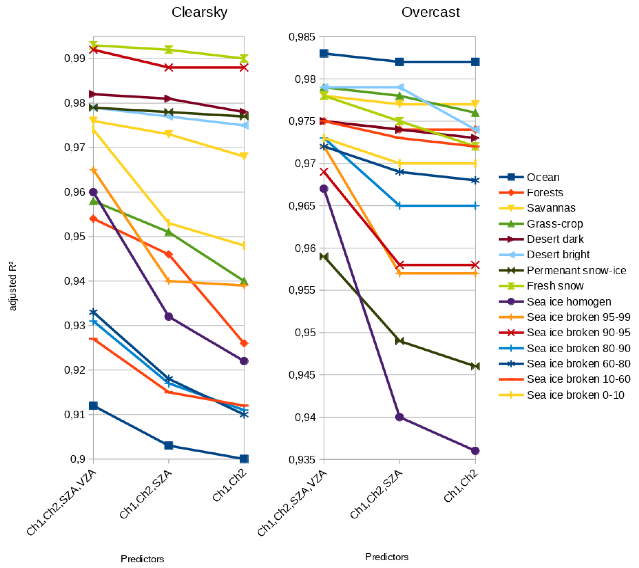
Multivariate linear regressions are performed for 15 surface types and 3 cloud cover classes, resulting in regression coefficients for 45 scene types. As a result, for each combination of AVHRR reflectances in channels 1 and 2, for a given scene type, a CERES-like broadband reflectance can be estimated. The linear regressions were found to be accurate, as demonstrated by the regression statistics: adjusted R 2 > 0.9 and relative RMS residual ( r R M S r ) below 3% for almost all clear-sky and overcast scene types, which is a significant improvement compared to previous works in the literature.
The added value of scene-dependent models was extensively demonstrated for regression calibration (better fit) as well as for validation (lower bias and r R M S r ). In addition, this study shows that the inclusion of solar and viewing zenith angle as predictors increases goodness-of-fit and lowers r R M S r , and furthermore proves necessary to avoid sampling-based model biases.
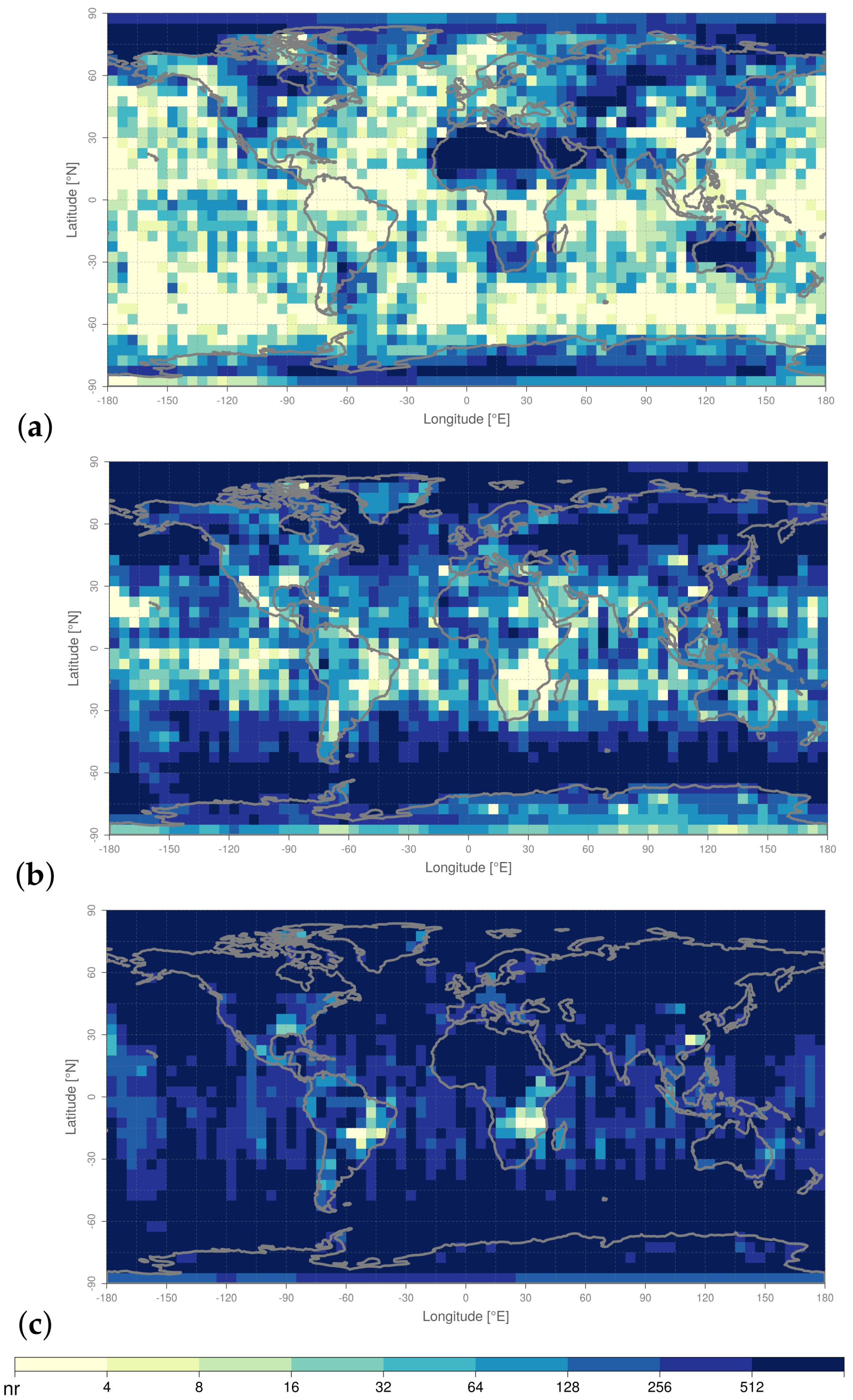
Validation of the regression models is done first by applying them on a validation subset (20% of pairs with strict matching criteria). The results indicate an overall good performance, with r R M S r similar to the calibration- r R M S r , and the flux-equivalent Mean Bias ( M B f l u x ) close to zero. A second validation approach makes use of a much expanded database with global coverage (obtained by relaxing matching criteria), allowing a spatially-explicit analysis and calculation of global mean statistics.
Error analysis is performed with three measures: Precision is given by the standard error of residuals, which is found very small (<0.03%). Stability is calculated by stratifying the data set according to the AVHRR-CERES instrument combination. The analysis reveals systematic instrument-specific biases with an order of (NOAAA19+Aqua) > (NOAA18+Aqua) > (NOAA17+Terra): this is illustrated by M B f l u x for all-sky conditions (+0.32, −0.86, −1.42 Wm 2 ), stressing the need for a well calibrated FCDR. Finally, accuracy is quantified as regional uncertainty at 1 standard deviation on a 5 × 5 grid (RMS bias), which is estimated for clear-sky and overcast conditions at respectively 1.8 and 2.3 Wm 2 (instantaneous); this corresponds with 0.7 and 0.9 Wm 2 on daily mean time scale, which is compliant with the GCOS requirements of 1 Wm 2 .

Author Contributions

T.A. wrote the paper which was thoroughly re-read by N.C. All authors have read and agreed to the published version of the manuscript.

Funding

This work was funded by the Climate Monitoring Satellite Application Facility (CM SAF) of EUMETSAT.

Acknowledgments

The authors are grateful to the Atmospheric Science Data Center at NASA Langley Research Center for providing the CERES data used in this work.

Conflicts of Interest

The authors declare no conflict of interest.

Abbreviations

The following abbreviations are used in this manuscript:
ADMAngular Dependency Model
AVHRRAdvanced Very High Resolution Radiometer
Ch1, Ch2Channel 1, Channel 2
CDRClimate Data Record
CERESClouds and the Earth’s Radiant Energy System (instrument and mission)
CZCSCoastal Zone Color Scanner
ECTEquatorial Crossing Time
ERBEarth Radiation Budget (instrument and mission)
ERBEEarth Radiation Budget Experiment (instrument and mission)
FCDRFundamental Climate Data Record
FMFlight Model
GACGlobal Area Coverage
GCOSGlobal Observing System for Climate
GERBGeostationary Earth Radiation Budget (instrument and mission)
GOESGeostationary Operational Environmental Satellite
IGBPInternational Geosphere-Biosphere Programme
LSTLocal solar time
MABMean absolute bias
MBMean bias
MB f l u x Flux-equivalent mean bias
MODISModerate Resolution Imaging Spectroradiometer
MSGMeteosat Second Generation
MVIRIMeteosat Visible and Infrared Imager
NOAA-XNational Oceanic and Atmospheric Administration, Satellite X
NTBNarrowband-to-Broadband
PSFPoint Spread Function
RMSRoot Mean Square
RMSrRoot Mean Square of residuals
RMSBRoot Mean Square of Biases
rRMSrrelative Root Mean Square of residuals
ScaRaBScanner for Radiation Budget
SErStandard Error of residuals
SEVIRISpinning Enhanced Visible and Infrared Imager
SSFSingle Scanner Footprint
SSRSum of Squared Residuals
SZASolar zenith angle
TOATop of Atmosphere
VISSRVisible-Infrared Spin-Scan Radiometer
VZAViewing zenith angle

Appendix A

Appendix A.1. Method: Data Preparation

The assumption of an at-nadir spherical CERES footprint with 32 km diameter was supported by sensitivity tests on a subset of the database, with pixel diameters of 20, 26, 32, 38 and 44 km respectively. For each configuration the rRMSr was calculated, and the 32 km configuration resulted in the lowest rRMSr.

Appendix A.2. Regression Calibration

Figure A1. R a d j 2 per scene type as function of regression predictors, for (a) clearsky and (b) overcast conditions.
Remotesensing 12 00305 g0a1

Appendix A.3. Validation: On Smaller Subset of Data

Table A1. Generic surface-type-independent regression performance based on smaller validation subset (20% of the observations with strict matching criteria), stratified per surface type, for clear, overcast, and allsky conditions; Data: 2004–2005 (NOAA17+Terra), 2007–2008 (NOAA18+Aqua) and 2011–2012 (NOAA19+Aqua).
Clear-SkyOvercastAll-Sky
Surface Type MB flux MB rMB rRMSr MB flux MB rMB rRMSr MB flux MB rMB rRMSr
Ocean−0.31−0.015−0.28%7.16%+1.57 *+0.169 *+0.39% *3.78%−2.53 *−0.344 *−1.19% *6.46%
Forests+2.31 *+0.200 *+1.67% *4.64%+2.14+0.197+0.40%3.64%−3.55−0.368−1.22%6.25%
Savannas−5.09 *−0.480 *−3.41% *5.36%+7.05+0.571+1.45%5.67%+0.42+0.028+0.13%6.83%
Grass/crop−3.97 *−0.429 *−2.76% *4.91%+0.45−0.003−0.01%3.16%−3.70 *−0.450 *−1.50% *5.58%
Dark deserts−0.73−0.083−0.45%3.39%+3.67+0.316+0.67%3.58%+5.72 *+0.521 *+2.19% *6.31%
Bright deserts+1.88 *+0.164 *+0.55% *2.44%+12.62 *+1.176 *+2.55% *4.23%+17.30 *+1.594 *+5.19% *6.37%
Perm. snow/ice−0.07 *+0.110 *+0.18% *1.12%+1.44 *+0.368 *+0.60% *2.47%+7.97 *+1.609 *+2.66% *4.40%
Fresh snow+0.80+0.083+0.21%2.56%+2.61 *+0.400 *+0.80% *2.74%+3.14 *+0.511 *+1.21% *4.40%
Sea ice 100%−1.36 *−0.350 *−0.66% *1.44%−0.22−0.105−0.20%1.71%+2.81 *+0.637 *+1.21% *3.55%
Sea ice 95–99%−1.16 *−0.256 *−0.48% *1.34%−0.13−0.078−0.14%1.94%+1.43 *+0.315 *+0.60% *3.55%
Sea ice 90–95%−0.50+0.010+0.02%1.62%−0.27−0.063−0.11%2.07%−0.73−0.105−0.20%3.61%
Sea ice 80–90%−0.57−0.040−0.11%1.78%−1.61 *−0.298 *−0.56% *2.30%−2.86 *−0.518 *−1.08% *3.87%
Sea ice 60–80%−4.19 *−0.472 *−1.57% *3.38%−1.69 *−0.262 *−0.53% *2.50%−4.10 *−0.700 *−1.59% *4.12%
Sea ice 10–60%+0.15+0.246+1.44%8.80%−1.41−0.159−0.36%3.02%−5.48 *−0.782 *−2.07% *5.10%
Sea ice 0–10%+0.96 *+0.175 *+3.01% *6.83%−1.33−0.115−0.27%3.38%−6.87 *−1.018 *−2.85% *5.65%
M B f l u x : mean bias expressed as isotropic flux (Wm 2 ); rMB: relative mean bias; rRMSr: relative rms residual. * statistically significant on the 99% confidence level.

Appendix A.4. Validation: On Expanded Validation Database (With Relaxed Matching Criteria) and Regional Analysis

Table A2. Generic surface-type-independent regression performance based on expanded database (with relaxed matching criteria), stratified per surface type, for clear, overcast, and allsky conditions; Data: 2004–2005 (NOAA17+Terra), 2007–2008 (NOAA18+Aqua) and 2011–2012 (NOAA19+Aqua).
Clear-SkyOvercastAll-Sky
Aggregation Type MB flux MB rMB rRMSr MB flux MB rMB rRMSr MB flux MB rMB rRMSr
Ocean−1.29 *−0.106 *−1.92% *8.17%+0.10 *−0.015 *−0.04% *4.59%−3.74 *−0.499 *−1.66% *7.27%
Forests+2.05 *+0.196 *+1.58% *4.38%+1.76+0.152+0.31%4.01%−3.47 *−0.374 *−1.22% *6.68%
Savannas−4.59 *−0.431 *−3.01% *5.15%+6.97 *+0.564 *+1.38% *5.40%+0.54+0.042+0.19%7.05%
Grass/crop−4.06 *−0.430 *−2.73% *4.92%+0.45−0.016−0.03%3.62%−3.33 *−0.413 *−1.42% *6.11%
Dark deserts−1.40 *−0.136 *−0.73% *3.46%+3.19+0.264+0.56%4.05%+5.45 *+0.509 *+2.12% *6.46%
Bright deserts+2.46 *+0.210 *+0.70% *2.62%+12.91 *+1.229 *+2.69% *4.73%+18.13 *+1.654 *+5.38% *6.68%
Perm. snow/ice−0.30 *+0.067 *+0.11% *1.30%−0.11 *−0.042 *−0.07% *2.91%+7.24 *+1.424 *+2.35% *4.45%
Fresh snow+1.44 *+0.175 *+0.43% *2.84%+1.68 *+0.149 *+0.29% *3.16%+2.69 *+0.339 *+0.78% *4.71%
Sea ice 100%−0.83 *−0.222 *−0.42% *1.51%−0.19 *−0.085 *−0.16% *1.95%+2.93 *+0.671 *+1.28% *3.66%
Sea ice 95–99%−0.63 *−0.146 *−0.27% *1.45%−0.21 *−0.089 *−0.16% *2.14%+1.47 *+0.316 *+0.60% *3.68%
Sea ice 90–95%−0.19+0.076+0.16%1.72%−0.82 *−0.145 *−0.26% *2.29%−0.65 *−0.084 *−0.16% *3.81%
Sea ice 80–90%−0.64 *−0.047 *−0.13% *1.94%−2.23 *−0.378 *−0.71% *2.51%−2.88 *−0.510 *−1.06% *4.02%
Sea ice 60–80%−3.42 *−0.383 *−1.27% *3.25%−2.57 *−0.376 *−0.75% *2.78%−4.29 *−0.717 *−1.63% *4.35%
Sea ice 10–60%+0.45 *+0.247 *+1.46% *8.22%−2.61 *−0.323 *−0.73% *3.56%−5.74 *−0.837 *−2.25% *5.65%
Sea ice 0–10%+0.96 *+0.186 *+3.20% *7.54%−2.57 *−0.339 *−0.78% *3.99%−7.45 *−1.176 *−3.26% *6.33%
Global mean [ 1 ] −1.16−0.087−1.17%n.a. [ 2 ] +1.59+0.126+0.63%n.a. [ 2 ] −0.96−0.138+1.91%n.a. [ 2 ]
M B f l u x : mean bias expressed as isotropic flux (Wm 2 ); r M B : relative mean bias; r R M S r : relative rms residual. * statistically significant on the 99% confidence level. [ 1 ] After spatial aggregation of all NTB pairs on a 5 × 5 grid with area-weighting. [ 2 ] Since rRMSr is calculated with respect to all NTB pairs within that scene type, this metric cannot be globally aggregated.

Appendix A.5. Accuracy

Table A3. Global accuracy statistics from bias map, based on surface-type-independent regressions from expanded database (with relaxed matching criteria) for clear, overcast, and allsky conditions; Data: 2004–2005 (NOAA17+Terra), 2007–2008 (NOAA18+Aqua) and 2011–2012 (NOAA19+Aqua).
Clear-SkyOvercastAll-Sky
StatisticRegression Predictors MB flux MB MB flux MB MB flux MB
global RMSBCh1,Ch2,SZA,VZA2.410.2963.510.4205.500.786
Ch1,Ch2,SZA2.710.3453.490.4705.920.827
Ch1,Ch22.580.3945.900.6785.850.842
global MABCh1,Ch2,SZA,VZA1.810.2292.350.2954.250.588
Ch1,Ch2,SZA2.140.2732.330.3174.800.656
Ch1,Ch22.000.3024.170.5054.390.643
Global statistics: R M S B : root mean square of biases (Wm 2 ); M A B Mean of absolute biases (Wm 2 ). On pixel-level: M B f l u x : mean bias expressed as isotropic flux (Wm 2 ); MB: mean reflectance bias (Wm 2 ).

References

  1. GCOS. Systematic Observation Requirements for Satellite-based Products for Climate (2011 Update): Supplemental details to the satellite-based component of the “Implementation Plan for the Global Observing System for Climate in Support of the UNFCCC”. Reference document GCOS-154, WMO. 2011. Available online: https://public.wmo.int/en (accessed on 1 December 2019).
  2. Loeb, N.G.; Doelling, D.R.; Wang, H.; Su, W.; Nguyen, C.; Corbett, J.G.; Liang, L.; Mitrescu, C.; Rose, F.G.; Kato, S. Clouds and the earth’s radiant energy system (CERES) energy balanced and filled (EBAF) top-of-atmosphere (TOA) edition-4.0 data product. J. Clim. 2018, 31, 895–918. [Google Scholar] [CrossRef]
  3. Urbain, M.; Clerbaux, N.; Ipe, A.; Tornow, F.; Hollmann, R.; Baudrez, E.; Velazquez Blazquez, A.; Moreels, J. The CM SAF TOA radiation data record using MVIRI and SEVIRI. Remote Sens. 2017, 9, 466. [Google Scholar] [CrossRef] [Green Version]
  4. Heidinger, A.K.; Straka, W.C., III; Molling, C.C.; Sullivan, J.T.; Wu, X. Deriving an inter-sensor consistent calibration for the AVHRR solar reflectance data record. Int. J. Remote Sens. 2010, 31, 6493–6517. [Google Scholar] [CrossRef]
  5. Hollman, R.; Schlundt, C.; Finkensieper, S.; Raspaud, M.; Karlsson, K.G.; Stengel, M. Technical Report on AVHRR GAC FCDR generation. Technical Report Issue 1, Revision 0, ESA Cloud cci. 2017. Available online: http://www.esa-cloud-cci.org/sites/default/files/upload/Cloud_cci_RAFCDR_v1.0.pdf (accessed on 1 December 2019).
  6. Abel, P.; Gruber, A. An Improved Model for the Calculation of Longwave Flux at 11 um; NOAA: Silver Spring, MD, USA, 1979.
  7. Godøy, Ø.; Eastwood, S. Narrowband to Broadband Correction of NOAA/AVHRR Data; Research Note 68; Norwegian Meteorological Institute: Oslo, Norway, 2002; ISSN 03329879. [Google Scholar]
  8. Cess, R.D.; Potter, G.L. Narrow-and broad-band satellite measurements of shortwave radiation: Conversion simulations with a general circulation model. J. Clim. Appl. Meteorol. 1986, 25, 1977–1984. [Google Scholar] [CrossRef] [Green Version]
  9. Laszlo, I.; Gruber, A.; Jacobowitz, H. The relative merits of narrowband channels for estimating broadband albedos. J. Atmos. Ocean. Technol. 1988, 5, 757–773. [Google Scholar] [CrossRef] [Green Version]
  10. Davis, P.; Major, E.; Jacobowitz, H. An assessment of NIMBUS 7 ERB shortwave scanner data by correlative analysis with narrowband CZCS data. J. Geophys. Res. Atmos. 1984, 89, 5077–5088. [Google Scholar] [CrossRef]
  11. Li, Z.; Leighton, H. Narrowband to broadband conversion with spatially autocorrelated reflectance measurements. J. Appl. Meteorol. 1992, 31, 421–432. [Google Scholar] [CrossRef] [Green Version]
  12. Hucek, R.; Jacobowitz, H. Impact of scene dependence on AVHRR albedo models. J. Atmos. Ocean. Technol. 1995, 12, 697–711. [Google Scholar] [CrossRef] [Green Version]
  13. Clerbaux, N.; Bertrand, C.; Caprion, D.; Depaepe, B.; Dewitte, S.; Gonzalez, L.; Ipe, A. Narrowband-to-broadband conversions for SEVIRI. In Proceedings of the 2005 EUMETSAT Meteorological Satellite Conference, P46. Citeseer, Dubrovnik, Croatia, 19–23 September 2005; pp. 351–357. Available online: http://citeseerx.ist.psu.edu/viewdoc/download?doi=10.1.1.547.9828&rep=rep1&type=pdf (accessed on 1 December 2019).
  14. Minnis, P.; Harrison, E.F. Diurnal Variability of Regional Cloud and Clear-Sky Radiative Parameters Derived from GOES Data. Part III: November 1978 Radiative Parameters. J. Cllm. AdpI. Met. 1984, 23, 1033–1051. [Google Scholar] [CrossRef] [Green Version]
  15. Cheruy, F.; Kandel, R.; Duvel, J. Outgoing longwave radiation and its diurnal variation from combined ERBE and Meteosat observations: 1. Estimating OLR from Meteosat data. J. Geophys. Res. Atmos. 1991, 96, 22611–22622. [Google Scholar] [CrossRef]
  16. Trishchenko, A.; Li, Z. Use of ScaRaB measurements for validating a GOES-based TOA radiation product. J. Appl. Meteor. 1998, 37, 591–605. [Google Scholar] [CrossRef]
  17. Wydick, J.E.; Davis, P.A.; Gruber, A. Estimation of Broadband Planetary Albedo From Operational Narrowband Satellite Measurements; Technical Report NESDIS 27; NOAA: Oslo, Norway, 1987.
  18. Loeb, N.G.; Wielicki, B.A.; Doelling, D.R.; Smith, G.L.; Keyes, D.F.; Kato, S.; Manalo-Smith, N.; Wong, T. Toward optimal closure of the Earth’s top-of-atmosphere radiation budget. J. Clim. 2009, 22, 748–766. [Google Scholar] [CrossRef] [Green Version]
  19. Vesperini, M.; Fouquart, Y. Determination of broad-band shortwave fluxes from the Meteosat visible channel by comparison to ERBE(Earth Radiation Budget Experiment). Contrib. Atmos. Phys./Beitraege zur Physik der Atmosphaere 1994, 67, 121–131. [Google Scholar]
  20. Wu, X.; Sullivan, J.T.; Heidinger, A.K. Operational calibration of the Advanced Very High Resolution Radiometer (AVHRR) visible and near-infrared channels. Can. J. Remote Sens. 2010, 36, 602–616. [Google Scholar] [CrossRef]
  21. Li, Z.; Trishchenko, A. A study toward an improved understanding of the relationship between visible and shortwave measurements. J. Atmos. Ocean. Technol. 1999, 16, 347–360. [Google Scholar] [CrossRef]
  22. Minnis, P.; Smith, W.L., Jr.; DP, G.; JK, A. Cloud Properties Derived From GOES-7 for Spring 1994 ARM Intensive Observing Period Using Version 1.0. 0 of ARM Satellite Data Analysis Program; NASA Langley Research Center: Hampton, VA, USA, 1995.
  23. Feng, J.; Leighton, H. Broadband solar radiances from visible band measurements: a method based on ScaRaB observations and model simulations. Int. J. Remote Sens. 2005, 26, 5125–5148. [Google Scholar] [CrossRef]
  24. Suttles, J.T.; Green, R.N.; Minnis, P.; Smith, G.L.; Staylor, W.F.; Wielicki, B.A.; Walker, I.; Young, D.; Taylor, V.; Stowe, L. Angular Radiation Models for Earth-Atmosphere System. Volume 1: Shortwave Radiation; NASA Langley Research Center: Hampton, VA, USA, 1988.
  25. Loeb, N.G.; Manalo-Smith, N.; Kato, S.; Miller, W.F.; Gupta, S.K.; Minnis, P.; Wielicki, B.A. Angular distribution models for top-of-atmosphere radiative flux estimation from the Clouds and the Earth’s Radiant Energy System instrument on the Tropical Rainfall Measuring Mission satellite. Part I: Methodology. J. Appl. Meteorol. 2003, 42, 240–265. [Google Scholar] [CrossRef]
  26. Su, W.; Corbett, J.; Eitzen, Z.; Liang, L. Next-generation angular distribution models for top-of-atmosphere radiative flux calculation from CERES instruments: Methodology. Meas. Tech. 2015, 8, 611–632. [Google Scholar] [CrossRef] [Green Version]
  27. Wielicki, B.A.; Barkstrom, B.R.; Harrison, E.F.; Lee, R.B., III; Smith, G.L.; Cooper, J.E. Clouds and the Earth’s Radiant Energy System (CERES): An earth observing system experiment. Bull. Am. Meteorol. Soc. 1996, 77, 853–868. [Google Scholar] [CrossRef] [Green Version]
  28. Geier, E.; Green, R.; Kratz, D.; Minnis, P.; Miller, W.; Nolan, S.; Franklin, C. CERES data management system: Single Satellite Footprint TOA/surface fluxes and clouds (SSF) collection document, release 2, version 1, 212 pp. and appendixes, NASA Langley Res. Cent., Hampton, Va. Radiat. and Aerosol Branch, Atmos. Sci. Res., NASA Langley Res. Cent., Hampton, Va. Available online: http://asd-www.larc.nasa.gov/ceres/collect_guide/SSF_CG.pdf (accessed on 1 December 2019).
  29. Green, R.; Wielicki, B.A. CERES ATBD: Convolution of Imager Cloud Properties With CERES Footprint Point Spread Function (Subsystem 4.4); Algorithm Theoretical Basis Document; NASA Langley Research Center: Hampton, VA, USA, 1997.
  30. Cracknell, A.P. Advanced Very High Resolution Radiometer AVHRR; CRC Press: Boca Raton, FL, USA, 1997.
  31. SMHI. CM SAF Cloud, Albedo, Radiation Data Record, AVHRR-Based, Edition 2 (CLARA-A2): Cloud Fraction; Algorithm Theoretical Basis Document; Swedish Meteorological and Hydrological Institute: Folkborgsvagen, Sweden, 2016. [Google Scholar]
  32. Loveland, T.; Belward, A. The international geosphere biosphere programme data and information system global land cover data set (DISCover). Acta Astronautica 1997, 41, 681–689. [Google Scholar] [CrossRef]
  33. Loeb, N.G.; Kato, S.; Loukachine, K.; Manalo-Smith, N. Angular Distribution Models for Top-of-Atmosphere Radiative Flux Estimation from the Clouds and the Earth’s Radiant Energy System Instrument on the Terra Satellite. Part I: Methodology. J. Atmos. Ocean. Technol. 2005, 22, 338. [Google Scholar] [CrossRef]
  34. Pistone, K.; Eisenman, I.; Ramanathan, V. Observational determination of albedo decrease caused by vanishing Arctic sea ice. Proc. Natl. Acad. Sci. USA 2014, 111, 3322–3326. [Google Scholar] [CrossRef] [PubMed] [Green Version]
  35. Minnis, P.; Bedka, K.; Doelling, D.; Trepte, Q.; Bedka, S.; Yost, C.; Scarino, B.; Khlopenkov, K.; Hong, G.; Thieman, M.; et al. A CERES-Consistent Long-Term Cloud and Clear Sky Radiation Property Dataset Using AVHRR Observations; NASA Langley Research Center: Hampton, VA, USA, 2015.
Figure 1. Daytime equatorial crossing time for the relevant satellite sensors.
Remotesensing 12 00305 g001
Figure 2. Schematic overview of data preparation steps.
Remotesensing 12 00305 g002
Figure 3. Sampling number of matched NTB pairs with strict matching criteria for (a) clear, (b) overcast, and (c) all-sky conditions in 5 × 5 boxes.
Remotesensing 12 00305 g003
Figure 4. Flux-equivalent Mean Bias ( M B f l u x ) between observed and estimated broadband reflectance, for overcast conditions; estimated values are calculated by applying surface-type-dependent regressions on the narrowband observations, using the predictors: (a) channels 1 + 2, (b) channels 1 + 2 and SZA, and (c) channels 1 + 2, SZA and VZA. Biases are calculated on expanded validation database (with relaxed matching criteria).
Remotesensing 12 00305 g004
Figure 5. Flux-equivalent Mean Bias ( M B f l u x ) between observed and estimated broadband reflectance, for (a) clear-sky and (b) all-sky conditions; estimated values are calculated by applying surface-type-dependent regressions on the narrowband observations, using all predictors (full regression model). Biases are calculated on expanded validation database (with relaxed matching criteria).
Remotesensing 12 00305 g005
Figure 6. Satellite-specific flux-equivalent Mean Bias ( M B f l u x , s a t ) between observed and estimated broadband reflectance, for all-sky conditions; estimated values are calculated by applying surface-type-dependent regressions on the narrowband observations. Biases are calculated on expanded validation database (with relaxed matching criteria), narrowed down to each of the satellite combinations (a) NOAA17/Terra, (b) NOAA19/Aqua, (c) NOAA18/Aqua; grid boxes with less than 32 observations are excluded and appear white in the maps.
Remotesensing 12 00305 g006
Table 1. Specifications for database with matched NTB pairs.
AVHRR
Satellite
CERES
Satellite
ECT (dir) 1 Analysis Period
(From–To)
Nr. of All-Sky
NTB Pairs 2
NOAA-17Terra~10:30 LST (D)1/5/2004–30/8/200517.106.331
NOAA-18Aqua~13:30 LST (A)1/7/2007–30/6/200814.256.034
NOAA-19Aqua~13:30 LST (A)1/7/2011–30/6/201214.395.121
1 Equatorial Crossing Time (ECT) as Local Solar Time (LST); flight direction (D = descending, A = ascending). 2 After filtering for temporal and angular constraints.
Table 2. Surface types, corresponding IGBP categories, and number of matched NTB pairs (with strict matching criteria) for clear, overcast, and all-sky conditions; Data: 2004–2005 (NOAA17+Terra), 2007–2008 (NOAA18+Aqua) and 2011–2012 (NOAA19+Aqua).
Surface TypeIGBP CategoryNr. (Clear)Nr. (Overcast)Nr.(All)
Ocean1744,099396,552875,251
Forests1,2,3,4,5526511,14644,405
Savannas8,98498600628,295
Grass/crop6,10,11,12,13,1413,65119,62976,910
Dark deserts7,1827,548562861,340
Bright deserts16108,1468089191,645
Perm. snow/ice1567,76646,403196,854
Fresh snow1940,407102,128481,576
Sea ice 100%Not applicable35,09534,319130,282
Sea ice 95–99%46,67885,440272,354
Sea ice 90–95%11,09848,876118,266
Sea ice 80–90%12,73784,861197,343
Sea ice 60–80%628659,595135,770
Sea ice 10–60%539378,287144,676
Sea ice 0–10%9272220,499381,304
(total) 441,9391,207,4583,336,271
Table 3. Regression coefficients based on calibration subset (80% of the NTB pairs with strict matching criteria), stratified per surface type, for clear, overcast, and allsky conditions; Data: 2004–2005 (NOAA17+Terra), 2007–2008 (NOAA18+Aqua) and 2011–2012 (NOAA19+Aqua).
Clear-SkyOvercastAll-Sky
Surface Type b 0 b 1 b 2 b 3 b 4 b 0 b 1 b 2 b 3 b 4 b 0 b 1 b 2 b 3 b 4
Ocean1.8281.093−0.480−0.0710.5224.3410.3130.4410.7701.3392.9420.3330.4470.7161.113
Forests0.9700.5670.3791.2951.0813.9370.3760.3830.9131.3412.5720.4090.3710.9191.616
Savannas1.4190.4550.3942.2330.7323.0330.3790.3804.4041.4522.3880.4160.3712.2600.697
Grass/crop2.2170.4530.3501.2021.3653.9400.4160.3431.2151.8182.8290.4300.3480.8691.781
Dark deserts2.4270.3700.3711.3340.7383.2840.3000.4611.5651.6791.6910.4320.3561.5461.141
Bright deserts3.2410.3620.3381.4641.2470.9780.4020.3842.6091.0281.5910.5530.2072.4881.523
Perm. snow/ice6.4830.2120.480−0.4521.35814.7540.1710.463−1.1876.57920.2380.0780.468−1.7064.602
Fresh snow1.7010.2830.4381.4312.7962.4330.3410.4261.2613.1981.6380.3060.4511.1453.388
Sea ice 100%4.1500.2140.4980.1443.7137.1590.2900.4230.3434.75121.6050.1790.324−2.2206.527
Sea ice 95–99%7.6400.2180.451-0.4203.5749.2360.2430.450−0.1394.31912.5430.2810.343−0.8415.585
Sea ice 90–95%6.1880.2590.427−0.2483.22910.3010.2200.461−0.3194.00610.4020.1740.504−1.1284.658
Sea ice 80–90%2.9540.3720.3430.2992.4319.6140.2180.472−0.1073.5799.5900.0730.628−0.8034.028
Sea ice 60–80%2.5630.4460.2590.5402.3996.8200.2710.4540.3872.8044.9120.2150.5410.3343.020
Sea ice 10–60%2.6760.4620.2180.3334.4754.7940.2820.4720.4162.2013.2880.2630.5170.4122.536
Sea ice 0–10%1.8020.901−0.2510.2461.9914.5250.3140.4430.3722.5243.1690.3480.4330.4982.830
(generic *)2.5030.3360.3841.1721.7204.1260.3600.3940.9632.3272.9650.3900.3630.8872.810
b 0 , b 1 , b 2 , b 3 , b 4 : coefficients in Equation (2). (*) surface-type-independent regression, that combines all matched NTB pairs (regardless the surface type).
Table 4. Regression metrics based on calibration subset (80% of the NTB pairs with strict matching criteria), stratified per surface type, for clear, overcast, and all-sky conditions; Data: 2004–2005 (NOAA17+Terra), 2007–2008 (NOAA18+Aqua) and 2011–2012 (NOAA19+Aqua).
Clear-SkyOvercastAll-Sky
Surface Type R adj 2 RMSrrRMSrSEr R adj 2 RMSrrRMSrSEr R adj 2 RMSrrRMSrSEr
Ocean0.9120.264.82%0.0010.9831.593.71%0.0030.9901.695.85%0.002
Forests0.9540.332.74%0.0050.9751.763.60%0.0190.9871.755.83%0.009
Savannas0.9760.382.70%0.0050.9782.085.25%0.0300.9851.306.13%0.009
Grass/crop0.9580.493.13%0.0050.9791.523.11%0.0120.9901.505.00%0.006
Dark deserts0.9820.563.05%0.0040.9751.623.42%0.0240.9861.245.21%0.006
Bright deserts0.9790.672.26%0.0020.9791.423.08%0.0180.9731.023.32%0.003
Perm. snow/ice0.9790.520.86%0.0020.9591.242.02%0.0060.8801.782.94%0.004
Fresh snow0.9930.962.41%0.0050.9781.282.55%0.0040.9761.744.11%0.003
Sea ice 100%0.9600.551.04%0.0030.9670.801.49%0.0050.8711.382.63%0.004
Sea ice 95–99%0.9650.561.05%0.0030.9720.941.70%0.0040.9001.683.18%0.004
Sea ice 90–95%0.9920.661.39%0.0070.9691.021.85%0.0050.9341.753.37%0.006
Sea ice 80–90%0.9320.571.57%0.0060.9731.082.04%0.0040.9641.523.17%0.004
Sea ice 60–80%0.9340.732.45%0.0100.9721.202.41%0.0050.9721.523.44%0.005
Sea ice 10–60%0.9261.347.77%0.0200.9751.332.98%0.0050.9821.594.21%0.005
Sea ice 0–10%0.9740.233.90%0.0030.9731.423.30%0.0030.9841.644.59%0.003
(generic *)0.9980.732.05%0.0010.9821.443.05%0.0010.9851.934.91%0.001
R a d j 2 : adjusted coefficient of determination; R M S r : root-mean-square residual; r R M S r : relative RMSr. S E r : standard error of residuals. (*) surface-type-independent regression, that combines all matched NTB pairs (regardless the surface type).
Table 5. Surface-type-dependent regression performance based on smaller validation subset (20% of the NTB pairs with strict matching criteria), stratified per surface type, for clear, overcast, and allsky conditions; Data: 2004–2005 (NOAA17+Terra), 2007–2008 (NOAA18+Aqua) and 2011–2012 (NOAA19+Aqua).
Clear-SkyOvercastAll-Sky
Surface Type MB flux MB rMB rRMSr MB flux MB rMB rRMSr MB flux MB rMB rRMSr
Ocean−0.04−0.003−0.06%4.81%+0.06−0.004−0.01%3.73%−0.23−0.031−0.11%5.86%
Forests+0.17+0.015+0.12%2.79%+0.81+0.058+0.12%3.61%−0.16−0.020−0.07%5.82%
Savannas−0.07−0.007−0.05%2.66%−1.23−0.105−0.27%5.40%−0.06−0.007−0.03%6.11%
Grass/crop+0.01−0.001−0.01%3.15%+0.42+0.027+0.06%3.11%−0.26−0.026−0.09%5.02%
Dark deserts+0.04+0.003+0.02%3.07%+0.92+0.082+0.17%3.44%−0.09−0.014−0.06%5.18%
Bright deserts+0.22+0.020+0.07%2.26%−0.48−0.050−0.11%3.05%+0.01+0.002+0.01%3.25%
Perm. snow/ice−0.19−0.031−0.05%0.86%−0.09−0.007−0.01%2.01%+0.12+0.034+0.06%2.95%
Fresh snow−0.07−0.020−0.05%2.42%−0.30−0.046−0.09%2.56%+0.05+0.041+0.10%4.11%
Sea ice 100%+0.08+0.023+0.04%1.05%+0.08+0.023+0.04%1.50%−0.18−0.028−0.05%2.64%
Sea ice 95–99%−0.27−0.058−0.11%1.06%−0.22−0.043−0.08%1.72%−0.11−0.013−0.02%3.19%
Sea ice 90–95%−0.15−0.030−0.06%1.36%−0.31−0.058−0.11%1.84%+0.15+0.027+0.05%3.36%
Sea ice 80–90%−0.07−0.005−0.01%1.64%+0.10+0.006+0.01%2.06%+0.25+0.030+0.06%3.17%
Sea ice 60–80%−0.27−0.022−0.07%2.52%+0.34+0.045+0.09%2.40%+0.29+0.033+0.08%3.45%
Sea ice 10–60%+0.57+0.083+0.48%7.80%−0.19−0.036−0.08%2.95%+0.04−0.003−0.01%4.21%
Sea ice 0–10%+0.02−0.002−0.03%3.79%−0.05−0.019−0.05%3.31%+0.06+0.002+0.01%4.61%
M B f l u x : mean bias expressed as isotropic flux (Wm 2 ); rMB: relative mean bias; rRMSr: relative rms residual.
Table 6. Surface-type-dependent regression performance based on expanded database (with relaxed matching criteria), stratified per surface type, for clear, overcast, and allsky conditions; Data: 2004-2005 (NOAA17+Terra), 2007-2008 (NOAA18+Aqua) and 2011–2012 (NOAA19+Aqua).
Clear-SkyOvercastAll-Sky
Aggregation Type MB flux MB rMB rRMSr MB flux MB rMB rRMSr MB flux MB rMB c rRMSr
Ocean−0.78 *−0.078 *−1.42% *6.12%−1.09 *−0.155 *−0.36% *4.63%−1.14 *−0.147 *−0.49% *6.82%
Forests−0.12+0.002+0.02%3.30%+0.88+0.056+0.12%4.00%+0.17+0.007+0.02%6.32%
Savannas+0.64 *+0.058 *+0.41% *3.14%−0.10−0.007−0.02%5.14%+0.39+0.035+0.16%6.57%
Grass/crop−0.24−0.026−0.17%3.38%+0.39+0.013+0.03%3.60%+0.04−0.007−0.03%5.62%
Dark deserts−0.69 *−0.062 *−0.33% *3.27%+0.19+0.004+0.01%3.95%−0.20−0.016−0.07%5.57%
Bright deserts+0.12+0.005+0.02%2.38%+0.42+0.042+0.09%3.72%−0.24−0.025−0.08%3.52%
Perm. snow/ice−0.64 *−0.116 *−0.19% *1.09%−0.59 *−0.179 *−0.29% *2.53%−0.62 *−0.169 *−0.28% *3.33%
Fresh snow+0.18+0.010+0.02%2.64%−0.42 *−0.144 *−0.28% *2.99%−0.64 *−0.155 *−0.36% *4.43%
Sea ice 100%+0.22 *+0.047 *+0.09% *1.11%−0.33−0.054−0.10%1.73%−0.11−0.013−0.02%2.88%
Sea ice 95–99%−0.03−0.018−0.03%1.16%−0.01+0.003+0.00%1.93%−0.08−0.008−0.01%3.34%
Sea ice 90–95%+0.01−0.004−0.01%1.47%−0.46 *−0.069 *−0.13% *2.08%−0.31 *−0.056 *−0.11% *3.58%
Sea ice 80–90%−0.09−0.018−0.05%1.75%−0.13−0.007−0.01%2.23%+0.20 *+0.047 *+0.10% *3.32%
Sea ice 60–80%+0.44 *+0.076 *+0.25% *2.46%−0.31−0.026−0.05%2.62%−0.30−0.031−0.07%3.63%
Sea ice 10–60%+1.20 *+0.151 *+0.89% *7.62%−0.93 *−0.125 *−0.28% *3.43%−0.62 *−0.092 *−0.25% *4.67%
Sea ice 0–10%+0.22+0.018+0.31%4.67%−1.09 *−0.206 *−0.47% *3.86%−0.93 *−0.191 *−0.53%*5.16%
Global mean [ 1 ] −0.81−0.085−1.19%n.a. [ 2 ] −0.08−0.044+0.19%n.a. [ 2 ] −0.64−0.092+0.64%n.a. [ 2 ]
M B f l u x : mean bias expressed as isotropic flux (Wm 2 ); rMB: relative mean bias; rRMSr: relative rms residual. * statistically significant on the 99% confidence level. [ 1 ] After spatial aggregation of all NTB pairs on a 5 ×5 grid with area-weighting. [ 2 ] Since rRMSr is calculated with respect to all NTB pairs within that scene type, this metric cannot be globally aggregated.
Table 7. Global stability statistics from bias map, based on expanded database (with relaxed matching criteria) for clear, overcast, and allsky conditions; Validation data is stratified per satellite combination, i.e., 2004–2005 (NOAA17+Terra), 2007–2008 (NOAA18+Aqua) and 2011–2012 (NOAA19+Aqua).
Clear-SkyOvercastAll-Sky
StatisticValidation Subset MB flux MB MB flux MB MB flux MB
global mean
(on 5 × 5 grid)
NOAA17+Terra−0.78−0.108+0.66+0.027+0.32+0.013
NOAA19+Aqua−0.50−0.017−0.41−0.063−0.86−0.087
NOAA18+Aqua−0.74−0.126−1.20−0.195−1.42−0.241
M B f l u x : mean bias expressed as isotropic flux (Wm 2 ); MB: mean reflectance bias (Wm 2 ).
Table 8. Global accuracy statistics from bias map, based on surface-type-dependent regressions from expanded database (with relaxed matching criteria) for clear, overcast, and allsky conditions; Data: 2004–2005 (NOAA17+Terra), 2007–2008 (NOAA18+Aqua) and 2011–2012 (NOAA19+Aqua).
Clear-SkyOvercastAll-Sky
StatisticRegression Predictors MB flux MB MB flux MB MB flux MB
global RMSBCh1,Ch2,SZA,VZA1.820.2172.290.3012.070.317
Ch1,Ch2,SZA1.960.2622.610.4652.390.429
Ch1,Ch22.090.2773.210.4872.330.427
global MABCh1,Ch2,SZA,VZA1.380.1681.760.2361.580.225
Ch1,Ch2,SZA1.550.2061.970.3001.860.294
Ch1,Ch21.600.2092.380.3481.770.297
Global statistics: R M S B : root mean square of biases (Wm 2 ); M A B Mean of absolute biases (Wm 2 ). On pixel-level: M B f l u x : mean bias expressed as isotropic flux (Wm 2 ); MB: mean reflectance bias (Wm 2 ).

