Article

Advantages of Uncombined Precise Point Positioning with Fixed Ambiguity Resolution for Slant Total Electron Content (STEC) and Differential Code Bias (DCB) Estimation

1
College of Geology Engineering and Geomatics, Chang’an University, Xi’an 710054, China
2
Department of Geomatics Engineering, University of Calgary, Calgary, AB T2N 1N4, Canada
3
National Key Laboratory of Geo-Information Engineering, Xi’an 710054, China
4
Xi’an Research Institute of Surveying and Mapping, Xi’an 710054, China
*
Author to whom correspondence should be addressed.
Remote Sens. 2020, 12(2), 304; https://doi.org/10.3390/rs12020304
Submission received: 30 November 2019 / Revised: 14 January 2020 / Accepted: 15 January 2020 / Published: 17 January 2020
(This article belongs to the Special Issue Remote Sensing of Ionosphere Observation and Investigation)

Abstract

:
The determination of slant total electron content (STEC) between satellites and receivers is the first step for establishing an ionospheric model. However, the leveling errors, caused by the smoothed ambiguity solutions in the carrier-to-code leveling (CCL) method, degrade the performance of ionosphere modeling and differential code bias (DCB) estimation. To reduce the leveling errors, an uncombined and undifferenced precise point positioning (PPP) method with ambiguity resolution (AR) was used to directly extract the STEC. Firstly, the ionospheric observables were estimated with CCL, PPP float-ambiguity solutions, and PPP fixed-ambiguity solutions, respectively, to analyze the short-term temporal variation of receiver DCB in zero or short baselines. Then, the global ionospheric map (GIM) was modeled using three types of ionospheric observables based on the single-layer model (SLM) assumption. Compared with the CCL method, the slight variations of receiver DCBs can be obviously distinguished using high precise ionospheric observables, with a 58.4% and 71.2% improvement of the standard deviation (STD) for PPP float-ambiguity and fixed-ambiguity solutions, respectively. For ionosphere modeling, the 24.7% and 27.9% improvements for posteriori residuals were achieved for PPP float-ambiguity and fixed-ambiguity solutions, compared to the CCL method. The corresponding improvement for residuals of the vertical total electron contents (VTECs) compared with the Center for Orbit Determination in Europe (CODE) final GIM products in global accuracy was 9.2% and 13.7% for PPP float-ambiguity and fixed-ambiguity solutions, respectively. The results show that the PPP fixed-ambiguity solution is the best one for the GIM product modeling and satellite DCBs estimation.

Graphical Abstract

1. Introduction

Ionospheric delay is one of the main error sources in the positioning and navigation applications of global navigation satellite systems (GNSSs) [1,2,3,4]. Under normal solar activity, the ionospheric delay is usually up to tens of meters, but it may exceed more than 100 m with ionospheric scintillation. Over the past two decades, the international GNSS Service (IGS) ionospheric working group has routinely produced global ionospheric map products with the developing GNSS constellations and installation of ground-based GNSS receiver sites worldwide [5]. For ionosphere modeling, the influence of the ionospheric layer height in the thin layer ionospheric model is investigated [6] and an enhanced mapping function is proposed [7]. An improved empirical model is used for ionosphere modeling, considering the stochastic process of each satellite [8]. The higher-order ionospheric delay is also demonstrated to mitigate its effects on precise point positioning (PPP) during disturbed ionospheric conditions [9]. The two-layer ionospheric model is also proposed to better model the structure of the ionosphere [10]. Consequently, the different ionospheric models are demonstrated to assess their performance in single-frequency or multi-frequency PPP [11,12,13,14]. The real-time ionospheric delays corrections are used in faster PPP to shorten the convergence time and obtain the fixed-ambiguities solutions [15,16,17].
To establish the ionospheric modeling with GNSS, extraction of ionospheric observables is the first task [18,19,20]. Due to the frequency-dependent features, the ionospheric information obtained from GNSS technology is coupled with satellite and receiver differential code biases (DCBs) [21,22]. Consequently, the DCBs interferes with the estimation of accurate and absolute ionospheric total electron content (TEC), and the performance of positioning and timing. The geometry-free (GF) combination of carrier-phase smoothed code measurements, which is applied by the CODE, is commonly used to estimate the ionospheric observables [23]. The carrier-to-code leveling (CCL) method with carrier-phase smoothed code measurements reduces the code noise by an averaging process and avoids resolving ambiguities. However, the leveling errors, a type of error related to arcs created due to the multipath and short-term fluctuation of receiver biases, degrades the accuracy of ionospheric observables [22,24,25].
Due to the high precision of precise point positioning (PPP), the ionospheric observables can be directly extracted by the uncombined PPP (UPPP) method [26,27]. In [28], the UPPP method was used to avoid the leveling errors by using precise ambiguity estimation and multipath effects elimination. In [18], the real-time ionospheric total electron content (TEC) was monitored and modeled by the UPPP method, and an accuracy of 1 to 2 TECU (Total Electron Content Unit) and 0.4 ns for ionosphere and DCBs results was achieved, respectively.
Significant receiver DCB seasonal variations, which are correlated with the ambient environment, have been found [29], excepting the reason of solar cycle variability [30]. Furthermore, the strong correlation between the total electron content (TEC) and receiver DCB stability was demonstrated during a three-year period [31]. Receiver DCBs are not as stable as the GNSS transmitter DCBs and sometimes remarkable intraday variability is exhibited in leveling errors of ionospheric observables [32,33]. The short-term variation of receiver code bias is also presented on the leveling errors of a short baseline [19,26]. This variation is caused by many factors, for instance, the grounding of GPS equipment [34] and the environment temperature [32]. To eliminate the time-variating terms of receiver DCBs, a modified carrier-to-code leveling method is proposed to retrieve ionospheric observables [25]. A detailed study of receiver DCBs’ short-term variability should be done with high precision ionospheric observables.
In previous research, the ionospheric observables for ionosphere modeling and DCB estimation are based on the smoothed ambiguities or float-ambiguity solutions [18,28]. The double-difference fixed-ambiguity solutions are used to extract the precise ionospheric observables in regional ionosphere modeling [35]. The PPP AR has already achieved by the decoupled satellite clock (DSC) model [36], fractional cycle bias (FCB) model [37,38], and the integer recovery clock model [39]. An “integer-levelling” method, which attempted to fix the ambiguity with integer values from the carrier-phase smoothed code method using decoupled-clock products, was proposed to eliminate the leveling errors [40,41,42]. The FCB model is also adopted to fix geometry-free combination ambiguities with wide-lane fixed-ambiguity and ionospheric-free fixed-ambiguity ionospheric extraction [10,43,44]. However, these methods are also based on the CCL method with geometry-free carrier-phase observations. Compared with the above methods, the UPPP method is more flexible in estimating the precise ionospheric observables with ambiguity-fixed solutions, which can evidently reduce the leveling error effects of ionospheric observables. The reliable ambiguity resolution is a key issue to obtain precise ionospheric observables. However, less studies have been based on the ambiguity-fixed uncombined PPP.
In this study, we firstly present the mathematical models to estimate the ionospheric observables with the CCL and PPP method. The ambiguity resolution method, ionospheric modeling, and DCB estimation method are also presented. Thereafter, the data process strategy is introduced. The ionospheric observables were estimated with the CCL, PPP float-ambiguity, and PPP fixed-ambiguity solution methods, respectively. Three comprehensive global ionospheric map (GIM) products were produced. Then, the comprehensive analyzes of the accuracy of three GIM products were performed. Finally, we discuss the results and give some conclusions.

2. Methods

Firstly, the basic observation equation is presented. The code and phase measurements are used to obtain the ionospheric observables. In the CCL method, the receiver and satellite DCBs are coupled with STEC. Hence, in the uncombined PPP method, the ionospheric delays are estimated together, with the receiver and satellite DCBs as unknown parameters. There are no extra ionospheric corrections as constraints for estimating the ionospheric delay parameters.

2.1. Basic Code and Phase Observation Equation

The dual-frequency code and phase measurement are described as [45]:
{ P r , f s = ρ + c ( d t r d t s ) + T + γ f I 1 + d r , f d f s + ε P , f L r , f s = ρ + c ( d t r d t s ) + T γ f I 1 + λ f N f + b r , f b f s + ε L , f ,
where P f is the code measurements at frequency f ( f = 1 , 2 ) (m), L f is the carrier phase measurement at frequency f ( f = 1 , 2 ) (m), ρ is the geometric range between receiver r and satellite s , c is the light speed, d t r is the receiver clock, d t s is the satellite clock, T is the slant troposphere delay, I 1 is the ionospheric delay along the line-of-sight of the receiver and satellite at the first frequency and γ f = λ f 2 / λ 1 2 , λ f is the wavelength at frequency f (cycle), N f is the phase ambiguity at frequency f , d r , f and d f s are the code biases at frequency f for the receiver and satellite, b r , f and b f s are the phase biases at frequency f for the receiver and satellite, and ε P , f and ε L , f include the multipath effect and measurement noise for the code and carrier phase.

2.2. Carrier-to-Code Leveling (CCL) Method

To remove the frequency-independent components, the geometry-free (GF) combination of code and phase measurements is formed by subtracting one frequency observable from the other frequency at the same satellite simultaneously. This geometry-free combination is the key foundation for acquiring the ionospheric information, as illustrated in the following [46]:
P r , 4 s = P r , 2 s P r , 1 s = ( γ 2 1 ) I 1 + D C B s D C B r + ε P 4 L r , 4 s = L r , 1 s L r , 2 s = ( γ 2 1 ) I 1 + ( λ 1 N 1 λ 2 N 2 ) + D P B r D P B s + ε L 4
where P r , 4 s and L r , 4 s is the geometry-free combinations for the code and phase measurement, D C B r = d r , 1 d r , 2 and D C B s = d 1 s d 2 s are the differential code biases for the receiver and satellite, and D P B r = b r , 1 b r , 2 and D P B s = b 1 s b 2 s are the differential phase biases for receiver and satellite.
In the CCL method, the phase measurement can be corrected by the averaged GF ambiguities. The carrier-phase smoothed code measurement can be formulated as:
L C C L = L 4 L 4 P 4 arc = ( γ 2 1 ) I 1 + ( D C B s D C B r ) + ε P 4
where L C C L denotes the ionospheric observables from the smoothed code measurements, L 4 P 4 arc = j = 1 n w j ( L r , 4 s , j P r , 4 s , j ) / j = 1 n w j , and w j is the elevation-angle-dependent weight to minimize the noise and multipath contribution of low elevation angles at epoch j for the arc with n observables.

2.3. Uncombined PPP with Ambiguity Resolution

With respect to the uncombined precise point positioning model, the ionospheric terms and the satellite and receiver DCBs can be estimated as unknowns [14,47]:
{ P r , f s = ρ + c ( d t ˜ r d t ˜ s ) + T + γ f I ˜ 1 + ε P , f L r , f s = ρ + c ( d t ˜ r d t ˜ s ) + T γ f I ˜ 1 + λ f N ˜ f + ε L , f ,
where the receiver and satellite clock offsets and ionospheric delay terms are reparametrized as d t ˜ r , d t ˜ s , and I ˜ 1 with the following equations:
{ d t ˜ r = d t r + γ 2 γ 2 1 d r , 1 + 1 1 γ 2 d r , 2 d t ˜ s = d t s + γ 2 γ 2 1 d 1 s + 1 1 γ 2 d 2 s I ˜ 1 = I 1 + 1 γ 2 1 ( D C B s D C B r ) N ˜ f = N f + b r , f b f s γ 2 + 1 γ 2 1 ( d r , 1 d 1 s ) + 2 γ 2 1 ( d r , 2 d 2 s ) .
It has been proven that the uncombined method is available for extracting the ionospheric observables and avoiding the effect of leveling errors [18,22,26,27]. Hence, the ionospheric observables obtained from uncombined PPP with float-ambiguity solutions are denoted as:
L U P P P = I ˜ 1 = I 1 + 1 γ 2 1 ( D C B s D C B r ) ,
where L U P P P is the ionospheric observable. However, the precision of ionospheric delay is mainly determined by the ambiguity resolution. In order to obtain further accuracy and reliable ionospheric observations, the uncombined precise point positioning with ambiguity resolution (PPP-AR) method is applied.
With the float ambiguities from the PPP in all stations in a network, the fractional cycle bias can be estimated [37,38]. With the estimated fractional cycle biases (FCBs) of phase ambiguities, B 1 s and B 2 s , the PPP model can be constrained with the virtual observations [48,49]:
{ N ˜ ( 1 , 1 ) = N ( 1 , 1 ) + ( B 1 B 2 ) N ˜ ( 4 , 3 ) = N ( 4 , 3 ) + ( 4 B 1 3 B 2 ) ,
where N ( 1 , 1 ) and N ( 4 , 3 ) are the integer ambiguities combination on each frequency; and N ˜ ( 1 , 1 ) and N ˜ ( 4 , 3 ) are the fixed-ambiguities combination, which are used to improve the PPP solutions.
So, with the fixed-ambiguity solutions, the ionospheric observables in Equation (6) can be further improved. Hence, we can obtain three types of ionospheric observables under different accuracy levels with the CCL method, PPP float-ambiguity solutions, and PPP fixed-ambiguity solutions. These ionospheric observables are used for ionosphere modeling in the following section.

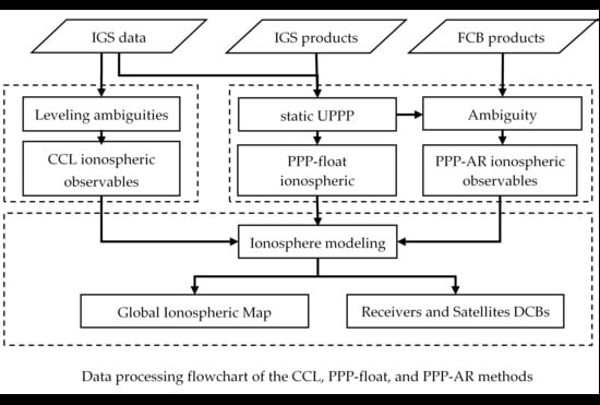
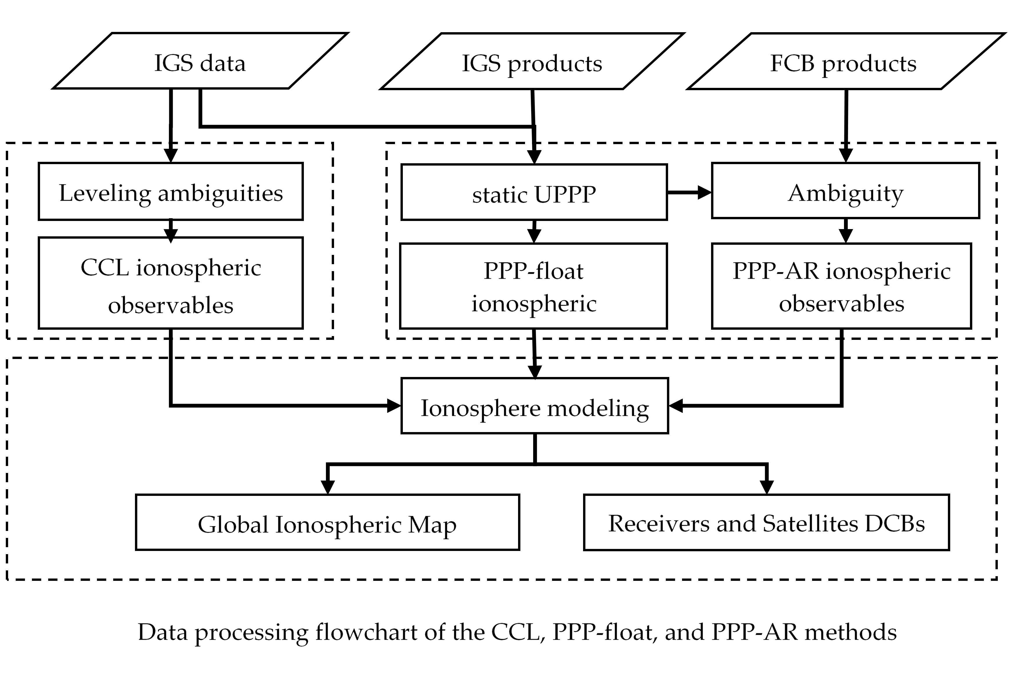
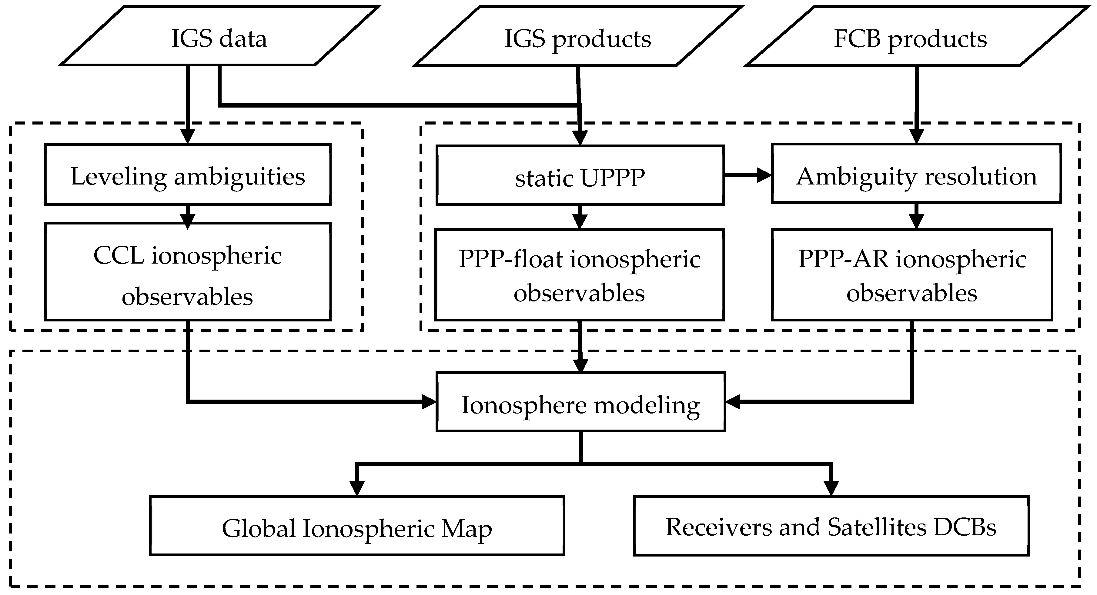
2.4. Ionospheric Modeling and Estimation of DCBs

From the above analysis, the two methods are introduced to obtain the ionospheric observables. Hence, three types solutions of ionospheric observables, CCL, PPP float-ambiguity solutions, and PPP fixed-ambiguity solutions, are used for ionosphere modeling in the following experiments and analysis. For the ionospheric observables L i o n , which are obtained in Equations (3) and (6) with float or fixed ambiguity solutions, the vertical TEC and differential code bias of receivers and satellites can be separated as:
L i o n = M F × K × V T E C ( φ i P P , λ i P P ) + 1 γ 2 1 ( D C B s D C B r ) ,
where M F = 1 / cos ( z ) is the modified mapping function, which is also adopted by CODE [2]; z is the zenith angle at the ionospheric pierce points (IPPs, unit: radian); V T E C is the vertical TEC, which is modeled as a general triangle series function (GTSF) of the latitude and local time; φ I P P and λ I P P are the latitude and longitude of the IPP; and D C B r and D C B s are the receiver and satellite DCBs, K = 40.3 × 10 16 / f 1 2 , with the frequency, f 1 .
The vertical ionospheric delay can be expressed using the spherical harmonic (SH) function for a period time of two hours or more [2,21]:
V T E C = n = 0 n max m = 0 n P ˜ n m sin ( φ I P P ) ( a n m cos ( m s ) + b n m sin ( m s ) ) ,
where P ˜ n m is the normalized, associated Legendre function of degree n and order m ; a n m and b n m are the unknown coefficients of the spherical harmonic function; n max is the maximum degree of spherical harmonic expansion; and s is the sun-fixed longitude of the ionospheric pierce point. With the ionospheric observables from all stations in a network, the coefficients of the spherical harmonic function, satellite, and receiver DCBs are estimated using the least square estimator. The satellite DCBs and receiver DCBs cannot be separated directly since these two types of parameters are linearly correlated. Hence, the general method using a forced mean zero constraint on satellite DCBs is adopted in ionosphere modeling [2].

3. Experiments and Results

In this section, we first describe the setup of the experiments, including the experimental environment, the datasets, and the processing strategies for uncombined PPP. Following this is a summary of the experimental results.

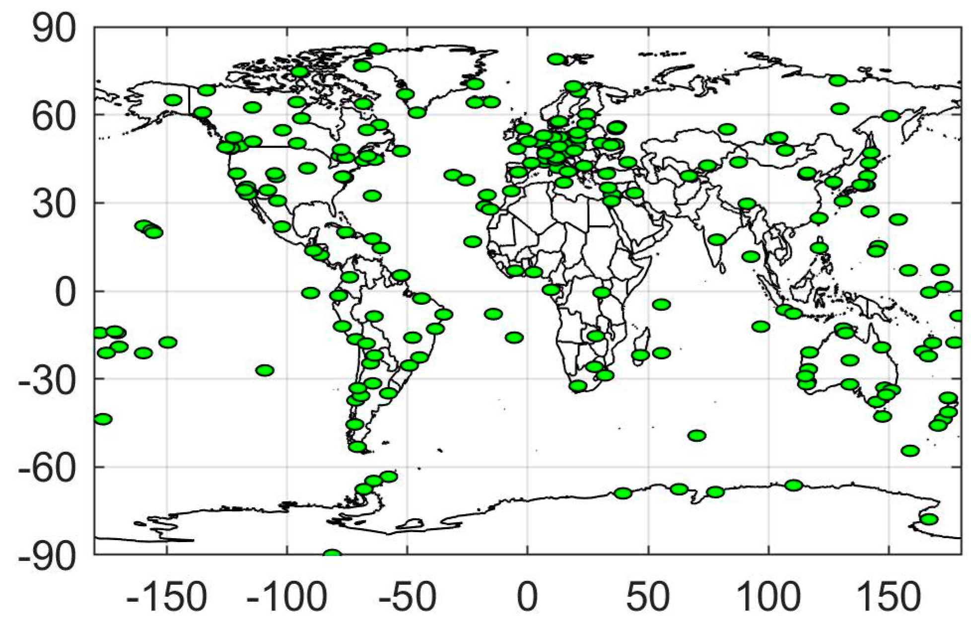
3.1. Experimental Setup

To evaluate the accuracy of ionospheric observables obtained from CCL, and the PPP float-ambiguity and PPP fixed-ambiguity solutions methods, the single differences between receivers’ ionospheric observables in zero or short baselines were performed with eight groups of stations in Table 1 on DOY (Day Of Year) 100, 2017: CUT0-CUT2, CUT0-CU3, EIL3-EIL4, and KOKB-KOKV, from four zero baselines, and LCK3-LCK4, YAR3-YARR, GODE-GODN, and WTZ3-WTZA, from four short baselines. In CCL, the ionospheric observables can be directly obtained by code and phase measurements. However, the ionospheric observables are estimated as unknown parameters in PPP methods. Hence, the detailed processing strategies for uncombined PPP methods are presented in Table 2.
For the accuracy assessment of the ionospheric observables in ionospheric modeling, three types of ionospheric observables were used to estimate the GIM products. The dataset of 268 stations on 10–16 April 2017 was collected from the IGS Global Data Center at CDDIS (Crustal Dynamics Data Information System, ftp://cddis.gsfc.nasa.gov/pub/gps/data/daily/2017/) to establish the global ionospheric map. Figure 1 shows the distributions of stations in the ionospheric modeling network. The CODE final GIM products were used to assess the performance of self-generated GIMs. Table 3 shows the details of the global ionosphere models. For convenient comparison, the carrier-to-code leveling method is called “CCL” and the PPP method with float ambiguity solutions is called “PPP-float” and the PPP method with fixed ambiguity resolution is called “PPP-AR”. Correspondingly, the ionosphere modeling results are also called “CCL”, “PPP-float”, and “PPP-AR” for the presentations.
The detailed data processing flowchart is presented in Figure 2. In the CCL method, the ionospheric observables were obtained by carrier and code measurements with leveling ambiguities while in the PPP method, they were directly estimated using the IGS precise orbit and clock products. With the FCB corrections, the ambiguity resolution of the PPP method was achieved, and ionospheric observables were estimated with the fixed-ambiguity solutions. Using three types of ionospheric observables, the global ionospheric map products were created with the modeling parameters in Table 3 using the same method in Equation (8). Compared with the CCL method, the ionospheric observables estimated from the PPP methods are more stable and accurate without the limitation of the arc length of the observables in CCL.

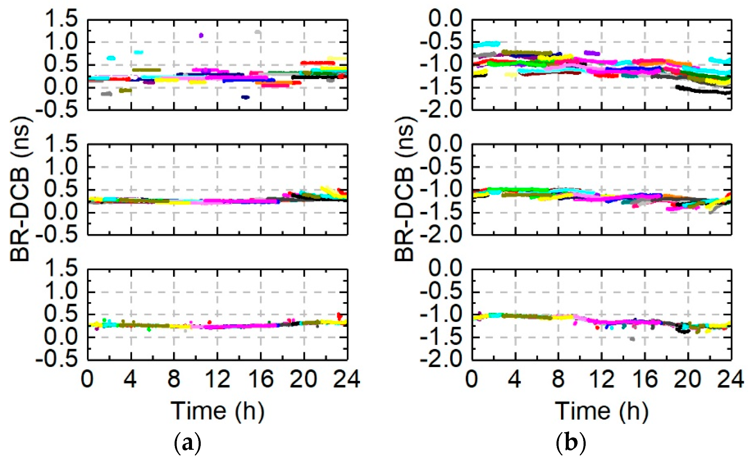
3.2. Accuracy of Ionospheric Observables

In order to assess the accuracy of the ionospheric observables, some co-located station pairs were selected to analyze the performance. For the zero baselines, CUT0-CUT2 and EIL3-EIL4 had the same receivers and CUT0-CUT3 and KOKB-KOKV had different receivers. For short baselines, LCK3-LCK4 were equipped with the same type of receivers and antennas. YAR3-YARR was equipped with the same type of receivers and different type of antennas. For GODE-GODN and WTZ3-WTZA, they had different receivers and different antennas. Here, CUT0-CUT2 and YAR3-YARR were selected to present the details of between-receiver DCB (BR-DCB) in Figure 3. The single difference of CUT0-CUT2 ranges from −0.16 to 0.9 ns for the CCL method and from 0.2 to 0.55 ns for the PPP-float and PPP-AR methods. Similarly, for YAR3-YARR, the single difference ranges from −1.65 to −0.53 ns for the CCL method and from −1.50 to −0.97 ns for the PPP-float and PPP-AR methods. The PPP method significantly improved the accuracy of ionospheric observables by reducing the leveling errors. For the averaged standard deviation (STD) of single-differenced ionospheric observables, it is 0.27 ns for the CCL method. The STDs were 0.11 and 0.07 ns for the PPP-float and PPP-AR methods, with 58.4% and 71.2% improvements, respectively, as shown in Table 4. Compared with the result of the float solutions, a 30.7% improvement could be achieved with the fixed ambiguity solutions. With fixed ambiguity resolution, the high precise ionospheric observables significantly reduced the leveling effects.
With the ambiguity resolution, we analyzed the performance in detecting the variations of BR-DCBs using the ionospheric observables in detail. For the CCL method, the averaged epoch STD was 0.272 and 0.311 ns while it was 0.067 and 0.068 ns in the PPP-float and 0.006 and 0.006 ns in the PPP-AR methods for KOKB-KOKV and WTZ3-WTZA, respectively, as shown in Figure 4. Hence, the high accuracy ionospheric observables, which were better than 0.01 ns (about 3 mm) with ambiguity resolution, can be used to detect the slight variations of single-difference receiver DCBs. As shown in Figure 4, for (a) and (d) panels, it is difficult to find the variations of BR-DCBs; however, significant variations can be seen in (b) and (e) for the PPP-float method and it can be definitively determined in the PPP-AR method, presented in the (c) and (f) panels. In the (c) panel, the BR-DCBs ranges from −4.68 to −4.76 ns in the initial period and then ranges from −4.76 to −4.48 ns. In the (f) panel, the BR-DCBs ranges from 16.12 to 16.23 ns and then ranges from 16.21 to 16.07 ns.

3.3. Ionospheric Modeling with Three Types of Ionospheric Observables

Ionospheric observables from 268 IGS stations, carried out with the CCL, PPP-float, and PPP-AR methods from DOY 100 to 106, 2017 (10–16 April 2017), were used for ionospheric modeling. The following section discusses the corresponding performance of self-generated GIM products.

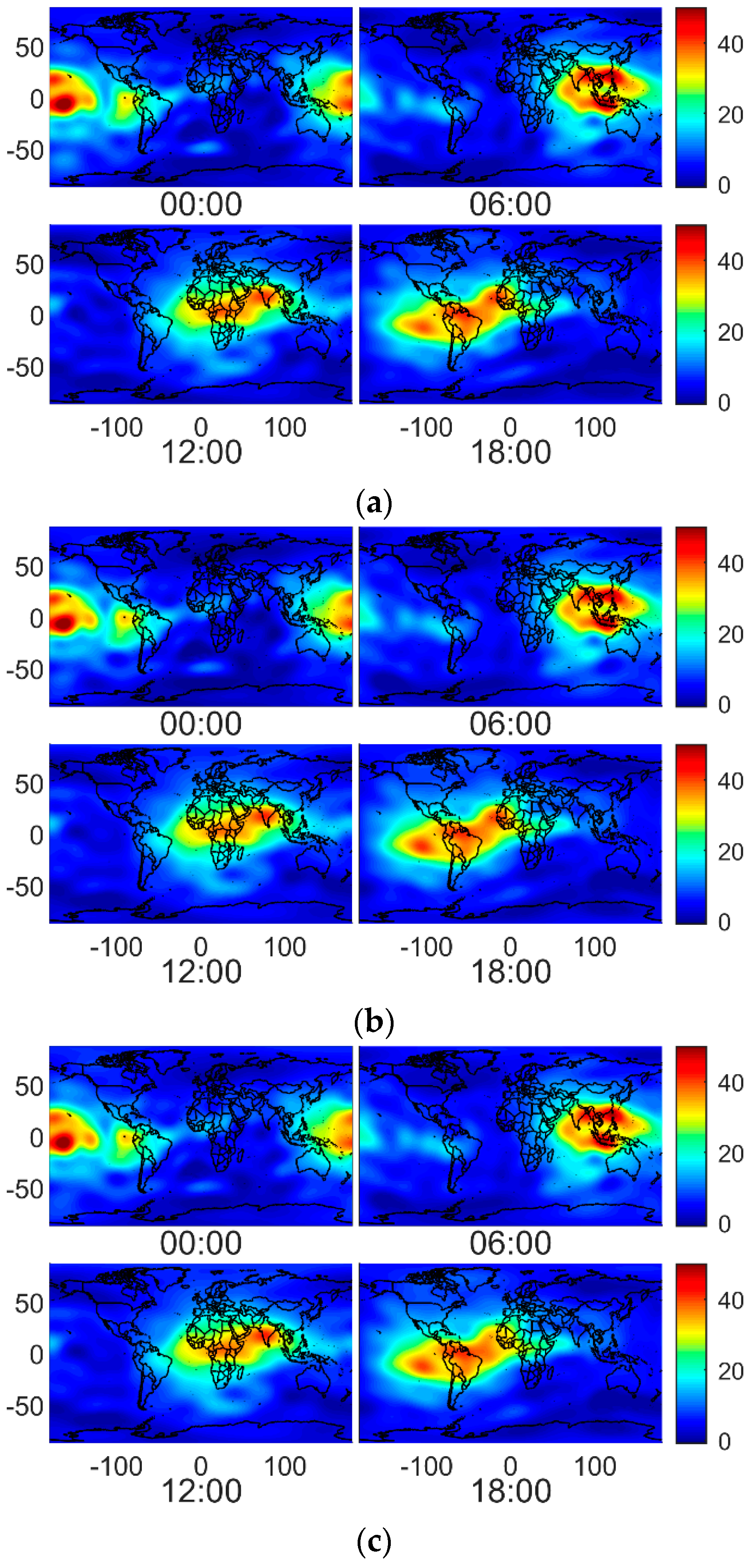
3.3.1. Self-Generated GIM Products

Figure 5 shows the ionospheric vertical total electron content (VTEC) in the global area at different times (0:00, 6:00, 12:00, 18:00) on DOY 100, 2017, with three different types of ionospheric observables. Excellent consistency can be found, which confirmed that ionospheric modeling with ionospheric observables estimated from the PPP method is a feasible method.

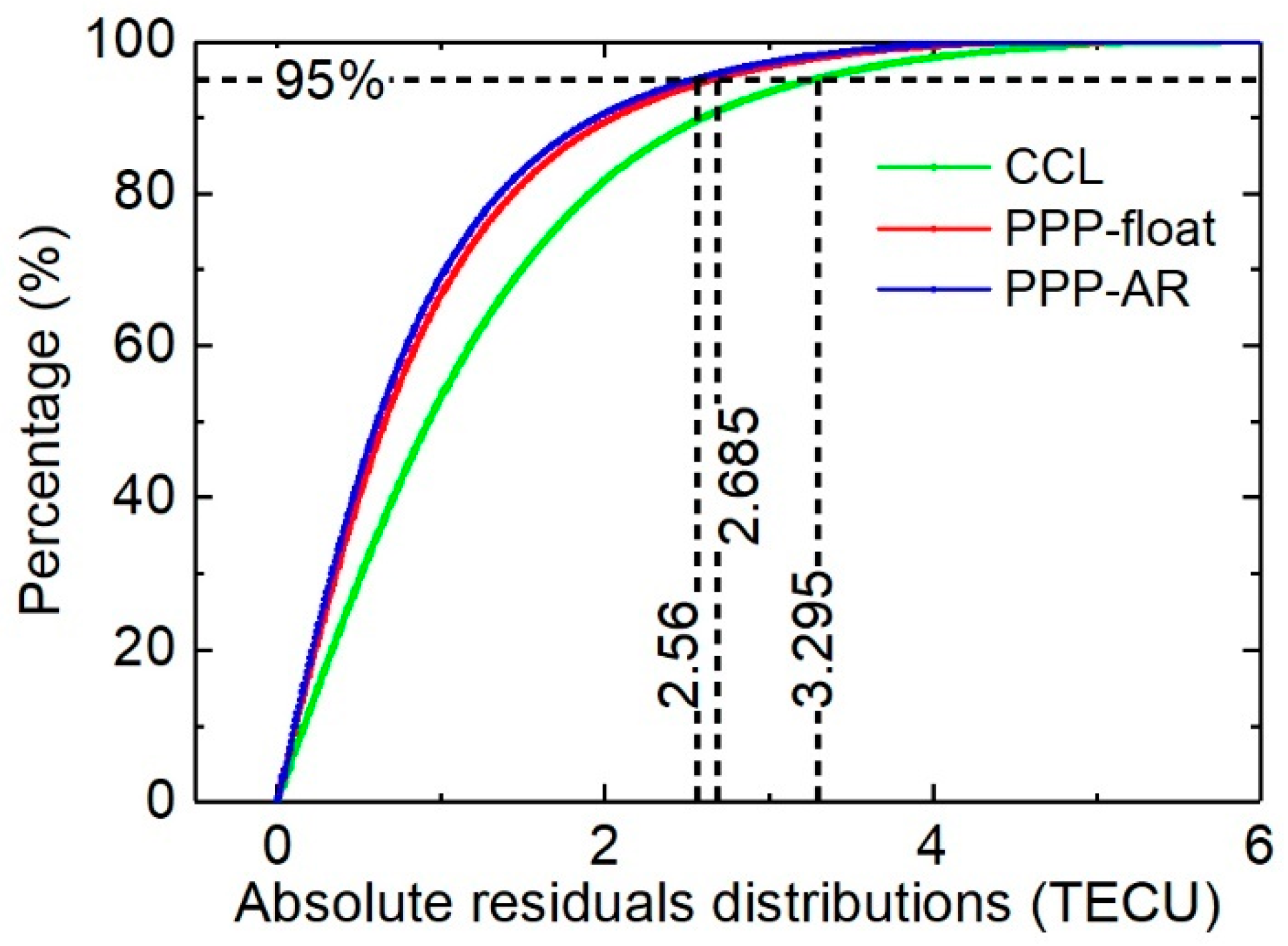
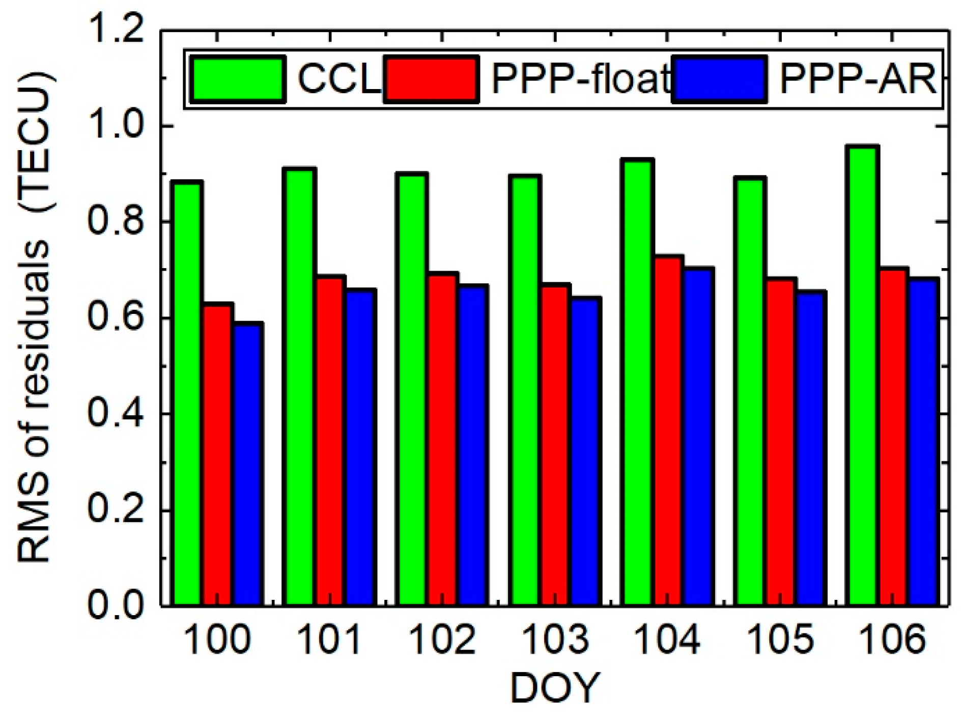
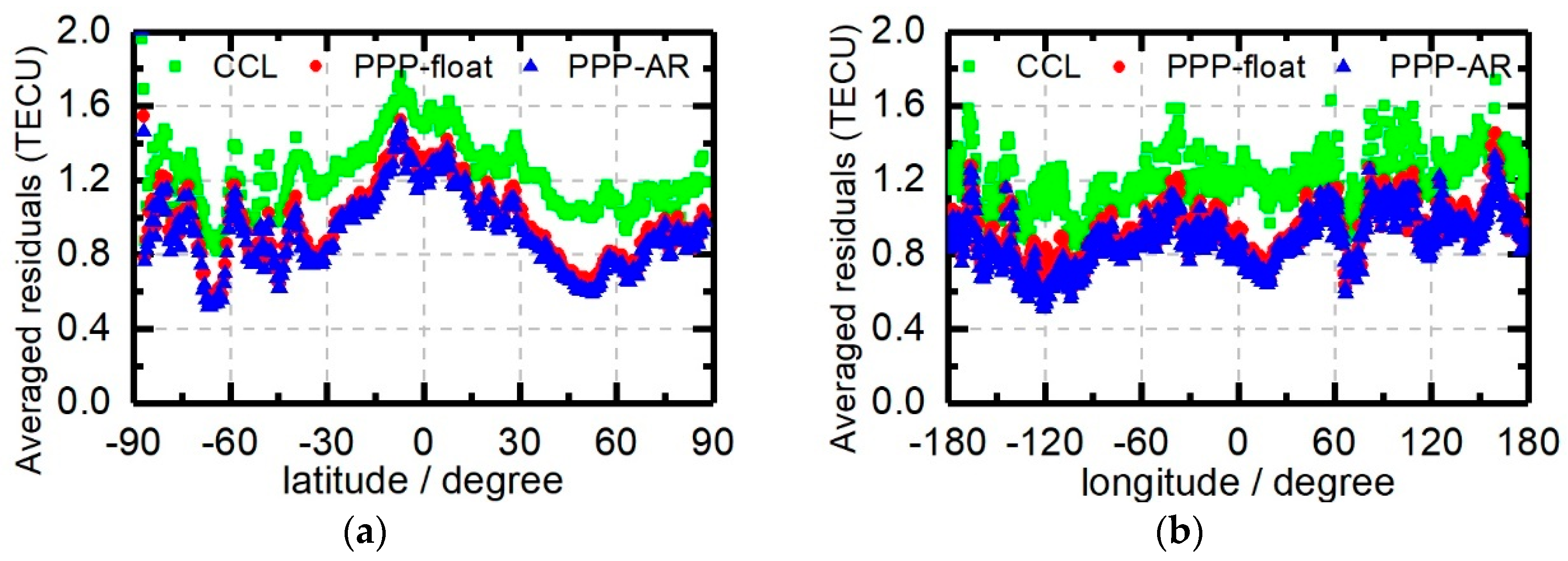
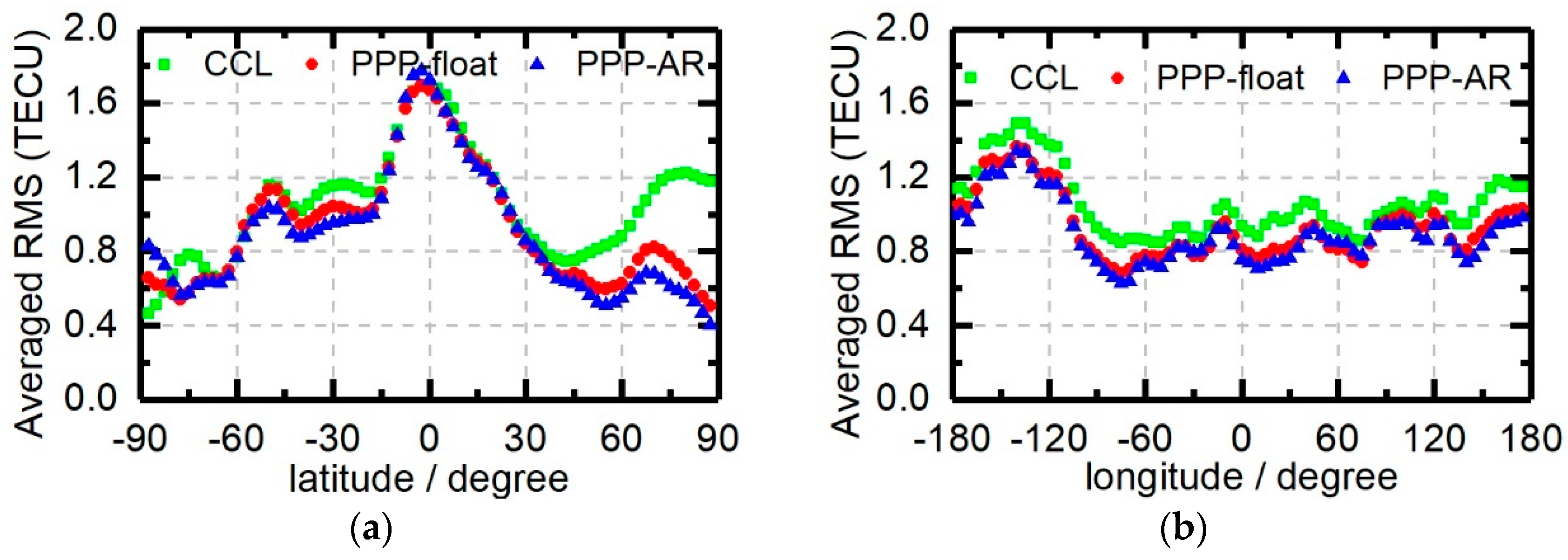
3.3.2. Accuracy of Ionospheric Observable Residuals

Figure 6 shows the posteriori residuals’ distribution of the ionospheric observables. All of the absolute residuals in one day were used for the frequency distributions. Although slight differences of the residual distributions are presented for the three types of results, most of their absolute residuals are less than 5 TECUs. Under the 95% confidence level, the threshold of ionospheric observable residuals is 2.56 TECUs for the PPP-AR method while it is 2.685 and 3.295 TECUs for the PPP-float and CCL methods, respectively. For the accuracy of RMS (Root Mean Square) of the posteriori residuals from ionospheric observables, 24.7% and 27.9% average improvements were achieved for the PPP-float and the PPP-AR methods compared to the CCL method with seven daily solutions from DOY 100 to 106, 2017, in Table 5. Furthermore, the RMSs of the ionospheric observables on each day are also presented in Figure 7. Although, the slight improvements for PPP-AR compared to PPP-float were achieved, PPP-AR showed the best performance, with significant improvements compared to the CCL method.
To further analyze the accuracy of the ionospheric modeling estimation, the latitude-dependent and longitude-dependent averaged residual distributions are shown in Figure 8. From the latitude-dependent averaged residuals, the values from −30 to 30 degrees are obviously larger than that in higher latitudes areas. It illustrated that the accuracy of ionospheric observables and modeling is affected by the ionosphere activity. Additionally, the variations in the southern hemisphere are larger than that of in the north hemisphere. This may be caused by the distributions’ gap of ionospheric observables. For longitude-dependent averaged residual distributions, it is relatively stable over all longitude areas, with some fluctuations as the shortage of observables. The significant improvement can be found for both of them in the PPP methods, especially in the PPP-AR method.

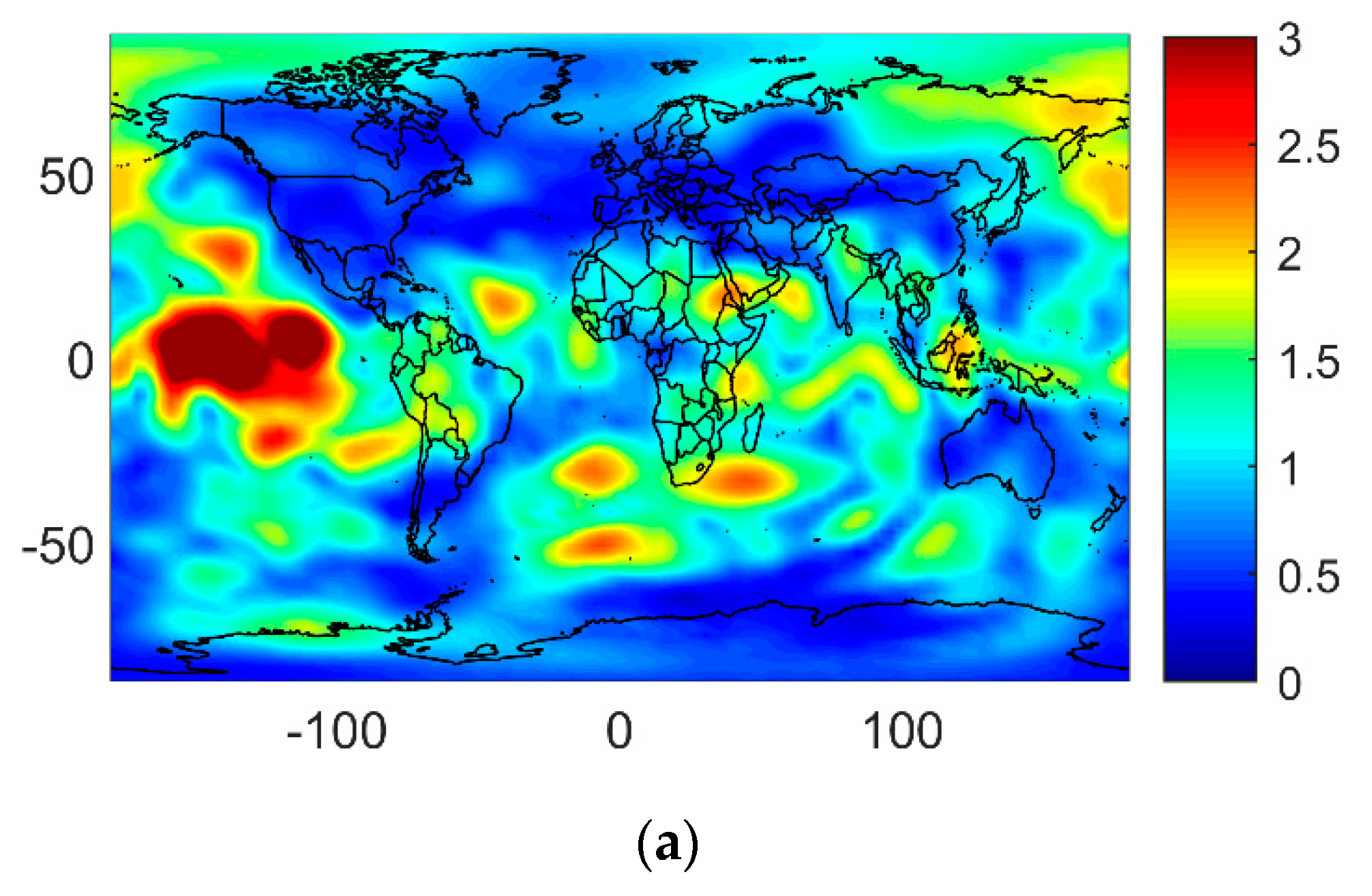
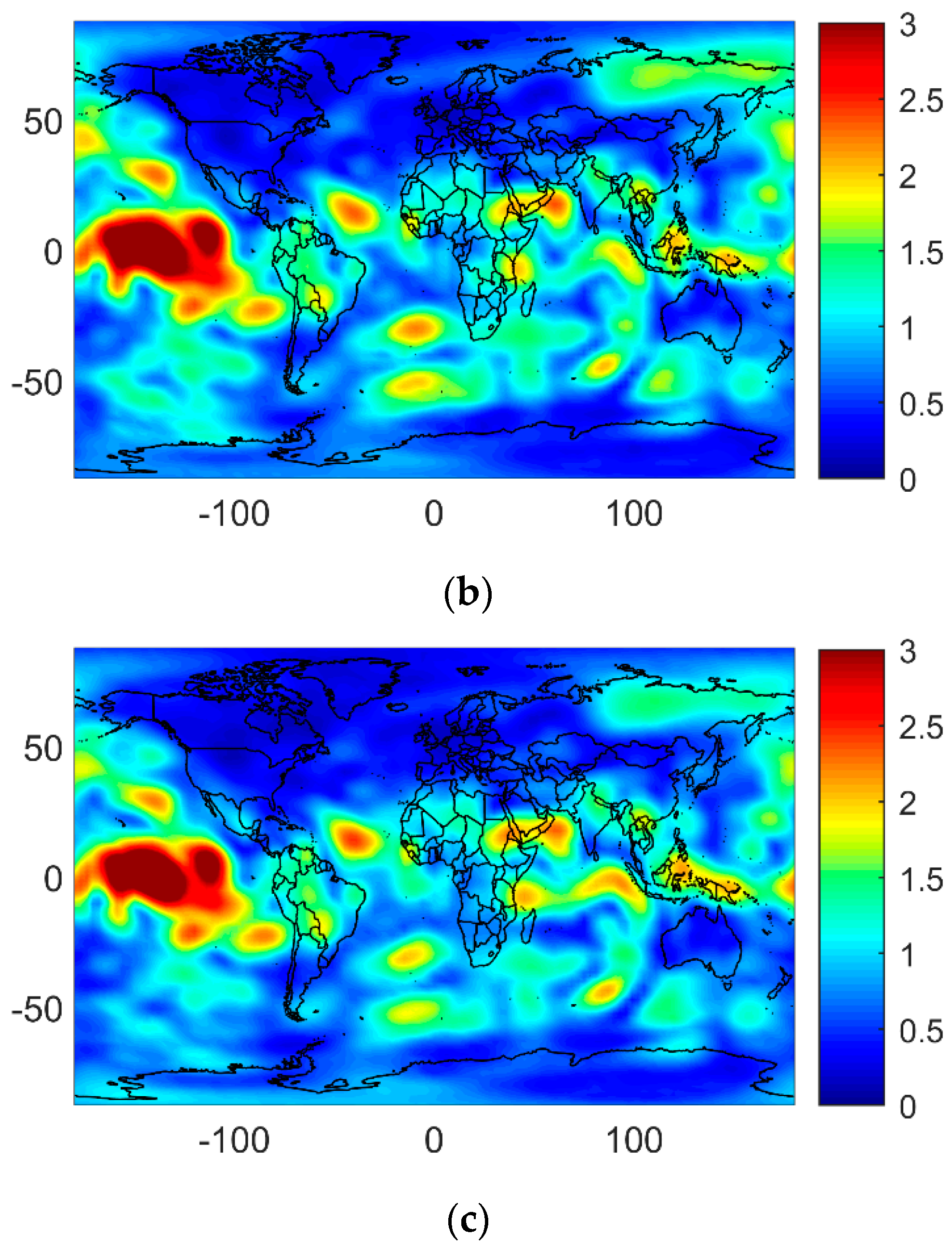
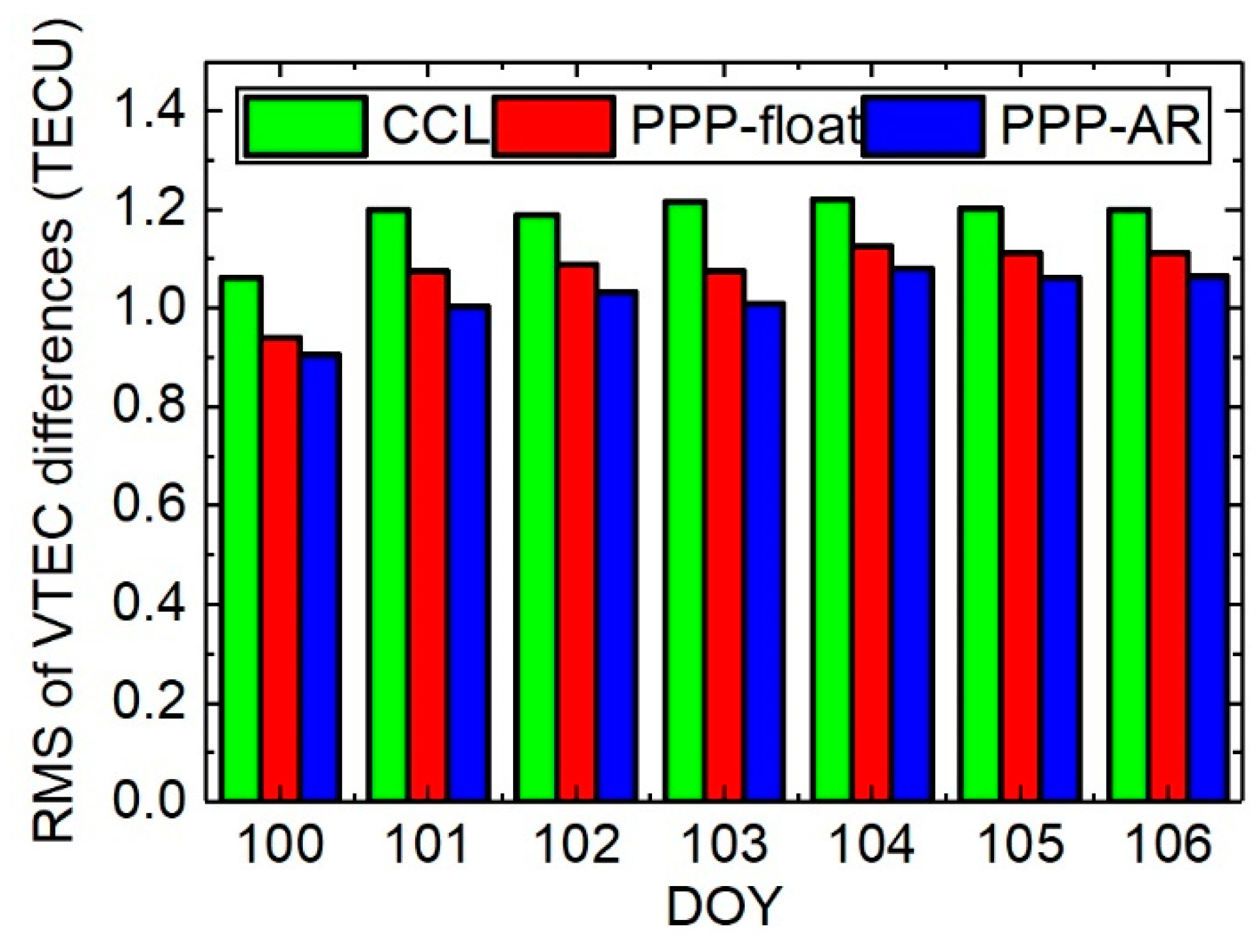
3.3.3. Comparison with CODE GIM Products

To assess the quality of self-generated VTEC products, the CODE final GIM products were used as the reference values. The CODE final GIM is a VTEC grid dataset in the IONosphere map Exchange (IONEX) format, with a resolution of 1 h, 5 degrees, and 2.5 degrees in time, longitude, and latitude, respectively. It was confirmed that the CODE final GIM product provides the VTEC grid with a high accuracy of two to eight TECU. The averaged differences between self-generated VTEC values and CODE VTEC values in one day period are presented in Figure 9. A significant improvement can be seen in north high latitude areas for PPP methods. For the RMS of differences compared with CODE GIM products, it is 1.05, 0.93, and 0.89 TECU for the CCL, PPP-float, and PPP-AR methods. A 9.2% and 13.7% average improvement was identified for the PPP-float and PPP-AR methods compared to the CCL method in Table 6. The detailed improvements on each day are presented in Figure 10 from DOY 100 to 106, 2017. With fixed ambiguity resolution, a slight improvement is achieved for RMS.
To analyze in detail the improvements for PPP-float, PPP-AR, and CCL, Figure 11 shows latitude-dependent and longitude-dependent averaged RMS distributions for the three techniques versus the CODE GIM model. In low latitude areas, the RMS is higher, and the technique shows a smaller effect, with a narrow spread between the three techniques. At high latitudes, the ambiguity-resolved PPP technique shows a clear improvement over the CCL and ambiguity float PPP techniques. It is about 1.65 TECU in the equator areas while it is about 0.8 TECU in high latitude areas. Especially, a significant improvement can be seen in northern hemisphere areas for the PPP-AR method compared with the CCL and PPP-float methods.

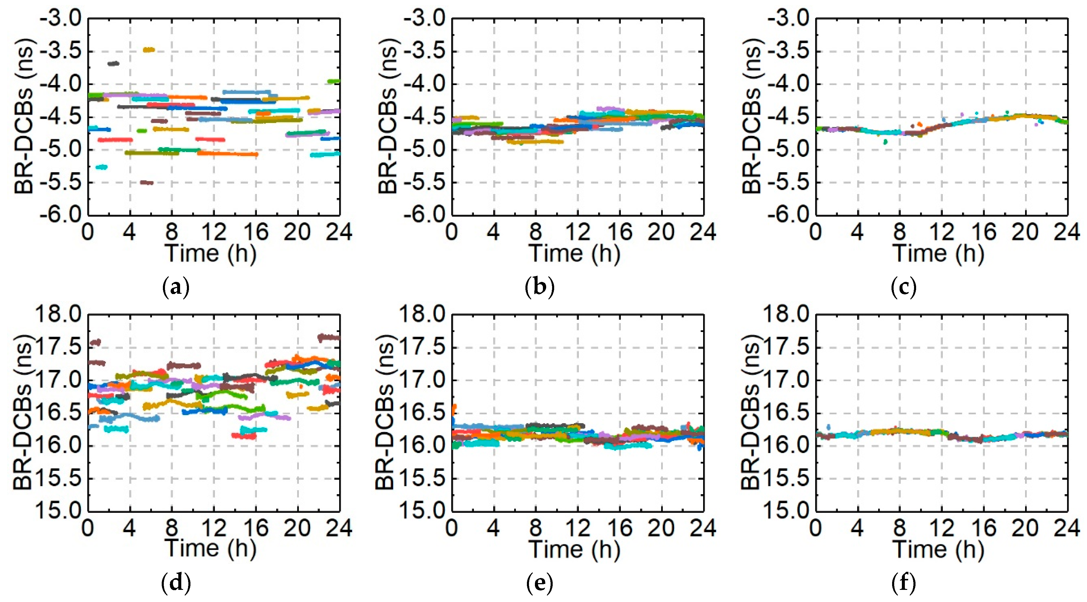
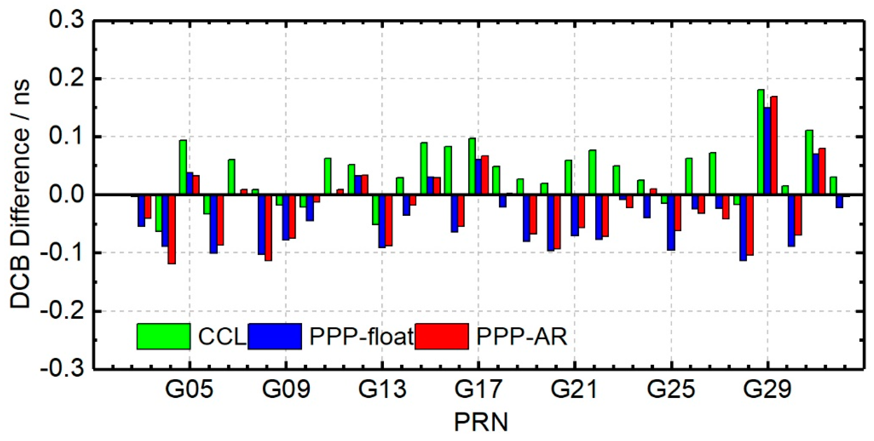
3.3.4. Satellites’ DCB Accuracy

In this experiment, the satellite DCBs were estimated together with ionospheric modeling from DOY 100 to 106, 2017. Compared with CODE final monthly satellite DCB products, the average daily biases are presented in Figure 12. Compared with the CCL method, more stable and accurate satellite DCB results were estimated with the PPP-float and PPP-AR methods. For the RMS, it is only 0.026 ns for the PP-AR methods and 0.035 ns for the PPP-float results in Table 7. Compared with the CCL methods, the improvements are 5.4% and 29.7% for the PPP-float and PPP-AR methods. With the fixed ambiguity resolution, 25.7% improvements were achieved for satellite DCB estimation compared to float ambiguity resolutions.

4. Discussion

The main interest of this study was the accuracy assessment of ionospheric observables obtained from the uncombined PPP with fixed ambiguity resolution and the corresponding ionosphere modeling. Excepting that the ionosphere modeling resolution can affect the performance, the measurement errors of ionospheric observables in reference stations is the main limitation in global ionospheric map corrections. The accuracy of ionospheric observables obtained from the CCL, PPP-float, and PPP-AR methods was firstly assessed by zero and short baseline experiments. With the fixed ambiguity resolution, the STD of single-differenced ionospheric observables is only about a quarter of that for CCL method. Compared with PPP-float solutions, 30.7% improvements were achieved for PPP-AR solutions. The undifferenced and uncombined PPP with fixed ambiguity resolution not only improves the performance of positioning but also improves the accuracy of ionosphere parameter estimation. For epoch solutions, the accuracy of ionospheric observables from PPP methods, removing the effects of the arc length and code measurement noise, is better than that of the CCL method. With high precision ionospheric observables, the slight variations of receiver DCBs is legible for an analysis of the receiver performances.
The experiments of ionospheric modeling with different ionospheric observables were processed to compare these with the CODE final GIM products. Consequently, high consistency of the self-generated GIMs products was achieved by the spherical harmonic model with both an order and degree of 15. From the distribution of residuals of ionospheric observables, the IPPs cover mainly areas over the world. However, the absence of stations in oceanic areas can affect the ionosphere modeling. The large residuals, mainly located in low latitude areas, indicate that the active ionosphere with high dynamic temporal and spatial variations degrades the accuracy of ionosphere modeling. This is another limitation that affects the accuracy of the ionospheric map corrections and it was not a focus in this study. Compared with CODE final GIM products, the results prove that the largest differences between self-generated and CODE-generated VTEC products are located in areas where there are no reference stations. A significant improvement was achieved in high latitude areas, especially in the northern hemisphere. As the coproducts of ionosphere modeling, the satellite DCB products were assessed compared with CODE final monthly products. A significant improvement was presented for PPP-AR compared with the PPP-float and CCL solutions. This implies that the fixed undifferenced carrier-phase ambiguities directly improved the estimation performance of ionosphere parameters in the uncombined PPP method.

5. Conclusions

An improved method to obtain the precise ionospheric observables was proposed for ionospheric modeling and the estimations of satellite and receiver DCBs using uncombined PPP with fixed ambiguity resolution. Obviously, the fixed undifferenced carrier phase ambiguities in PPP improves the estimation accuracy of coordinates and ionosphere parameters. The accuracy of ionospheric observables was confirmed by co-located stations in zero or short baselines. Significant improvements in the PPP-AR method were available to detect the slight variations of receiver DCBs. The accuracy within 0.01 ns for ionospheric observables helped us to study the receiver DCB and isolate it with the slant total electron content. In the PPP methods, the accuracy of the ionospheric observables is not limited by the arc length of the measurements.
Using the ionospheric observables from the three methods, CCL, PPP-float, and PPP-AR, the self-generated ionospheric map products were compared with CODE final GIM products. For the residuals of ionospheric observables, significant improvements were achieved for PPP methods, especially for PPP-AR. The highly precise ionospheric observables helped to generate precise ionospheric map corrections. Compared with CODE products, PPP-AR presented the best performance, with an RMS better than 1.022 TECU. The ionospheric observables were estimated from the uncombined PPP method in single stations with fixed undifferenced ambiguities, which shows a convenient method for real-time ionospheric modeling. The real-time PPP with ambiguity resolution was a realizable processing tool to generate real-time ionospheric corrections, which are crucial to support single-frequency PPP and PPP-RTK. However, the ionospheric scintillation effects on PPP should be treated cautiously in future work [50,51].

Author Contributions

J.W., G.H. and P.Z. conceived and designed the experiments; J.W. and G.H. performed the experiments, analyzed the data and wrote the paper; Y.Y., Q.Z. and Y.G. reviewed and improved the paper. All authors have read and agreed to the published version of the manuscript.

Funding

This research was funded by the National Key Research and Development Program of China (Grant No. 2018YFC1505102), the Programs of the National Natural Science Foundation of China (Grant No. 41774025, 41731066, 41904039), Special Fund for Technological Innovation Guidance of Shaanxi Province (Grant No. 2018XNCGG05), the Special Fund for Basic Scientific Research of Central Colleges (Grant No. CHD300102269305, CHD300102268305, Chang’an University), the Grand Projects of the Beidou-2 System (Grant No. GFZX0301040308) and the China Scholarship Council (award to Jin Wang for 2 year’s study abroad at the University of Calgary).

Acknowledgments

We thank the IGS and MGEX authorities for providing the data for this study.

Conflicts of Interest

The authors declare no conflict of interest.

References

  1. Klobuchar, J.A. Ionospheric Time-Delay Algorithm for Single-Frequency GPS Users. IEEE Trans. Aerosp. Electron. Syst. 1987, AES-23, 325–331. [Google Scholar] [CrossRef]
  2. Schaer, S. Mapping and Predicting the Earth’s Ionosphere Using the Global Positioning System. Ph.D. Thesis, Dissertation Astronomical Institute, University of Berne, Berne, Switzerland, 25 March 1999. [Google Scholar]
  3. Rovira-Garcia, A.; Juan, J.M.; Sanz, J.; Gonzalez-Casado, G. A Worldwide Ionospheric Model for Fast Precise Point Positioning. IEEE Trans. Geosci. Remote Sens. 2015, 53, 4596–4604. [Google Scholar] [CrossRef] [Green Version]
  4. Xu, G.; Xu, Y. GPS: Theory, Algorithms and Applications, 3rd ed.; Springer: Berlin, Germany, 2016; pp. 63–80. [Google Scholar]
  5. Hernández-Pajares, M.; Juan, J.M.; Sanz, J.; Orus, R.; Garcia-Rigo, A.; Feltens, J.; Komjathy, A.; Schaer, S.C.; Krankowski, A. The IGS VTEC maps: A reliable source of ionospheric information since 1998. J. Geod. 2009, 83, 263–275. [Google Scholar] [CrossRef]
  6. Brunini, C.; Camilion, E.; Azpilicueta, F. Simulation study of the influence of the ionospheric layer height in the thin layer ionospheric model. J. Geod. 2011, 85, 637–645. [Google Scholar] [CrossRef]
  7. Xiang, Y.; Gao, Y. An Enhanced Mapping Function with Ionospheric Varying Height. Remote Sens. 2019, 11, 1497. [Google Scholar] [CrossRef] [Green Version]
  8. Shi, C.; Gu, S.; Lou, Y.; Ge, M. An improved approach to model ionospheric delays for single-frequency Precise Point Positioning. Adv. Space Res. 2012, 49, 1698–1708. [Google Scholar] [CrossRef]
  9. Banville, S.; Sieradzki, R.; Hoque, M.; Wezka, K.; Hadas, T. On the estimation of higher-order ionospheric effects in precise point positioning. GPS Solut. 2017, 21, 1817–1828. [Google Scholar] [CrossRef]
  10. Nie, W.; Xu, T.; Rovira-Garcia, A.; Zornoza, J.; Subirana, J.; González-Casado, G.; Chen, W.; Xu, G. The Impacts of the Ionospheric Observable and Mathematical Model on the Global Ionosphere Model. Remote Sens. 2018, 10, 169. [Google Scholar] [CrossRef] [Green Version]
  11. Nie, W.; Hu, W.; Pan, S.; Wang, S.; Jin, X.; Wang, B. Application of Independently Estimated DCB and Ionospheric TEC in Single-Frequency PPP. In Lecture Notes in Electrical Engineering, Proceedings of the China Satellite Navigation Conference (CSNC) 2014 Proceedings, Nanjing, China, 21–23 May 2014; Sun, J., Jiao, W., Wu, H., Lu, M., Eds.; Springer: Berlin, Germany, 2014; Volume 304, p. 304. [Google Scholar]
  12. Wang, A.; Chen, J.; Zhang, Y.; Meng, L.; Wang, J. Performance of Selected Ionospheric Models in Multi-Global Navigation Satellite System Single-Frequency Positioning over China. Remote Sens. 2019, 11, 2070. [Google Scholar] [CrossRef] [Green Version]
  13. Su, K.; Jin, S.; Hoque, M.M. Evaluation of Ionospheric Delay Effects on Multi-GNSS Positioning Performance. Remote Sens. 2019, 11, 171. [Google Scholar] [CrossRef] [Green Version]
  14. Zhou, F.; Dong, D.; Li, W.; Jiang, X.; Wickert, J.; Schuh, H. GAMP: An open-source software of multi-GNSS precise point positioning using undifferenced and uncombined observations. GPS Solut. 2018, 22, 33. [Google Scholar] [CrossRef]
  15. Zhou, P.; Wang, J.; Nie, Z.; Gao, Y. Estimation and representation of regional atmospheric corrections for augmenting real-time single-frequency PPP. GPS Solut. 2020, 24, 7. [Google Scholar] [CrossRef]
  16. Zhang, L.; Yao, Y.; Peng, W.; Shan, L.; He, Y.; Kong, J. Real-Time Global Ionospheric Map and Its Application in Single-Frequency Positioning. Sensors 2019, 19, 1138. [Google Scholar] [CrossRef] [PubMed] [Green Version]
  17. Banville, S.; Collins, P.; Zhang, W.; Langley, R.B. Global and Regional Ionospheric Corrections for Faster PPP Convergence. Navigation 2014, 61, 115–124. [Google Scholar] [CrossRef]
  18. Tu, R.; Zhang, H.; Ge, M.; Huang, G. A real-time ionospheric model based on GNSS Precise Point Positioning. Adv. Space Res. 2013, 52, 1125–1134. [Google Scholar] [CrossRef]
  19. Zhang, B.; Teunissen, P.J.G.; Yuan, Y. On the short-term temporal variations of GNSS receiver differential phase biases. J. Geod. 2017, 91, 563–572. [Google Scholar] [CrossRef] [Green Version]
  20. Brunini, C.; Azpilicueta, F. GPS slant total electron content accuracy using the single layer model under different geomagnetic regions and ionospheric conditions. J. Geod. 2010, 84, 293–304. [Google Scholar] [CrossRef]
  21. Wang, N.; Yuan, Y.; Li, Z.; Montenbruck, O.; Tan, B. Determination of differential code biases with multi-GNSS observations. J. Geod. 2016, 90, 209–228. [Google Scholar] [CrossRef]
  22. Xiang, Y.; Gao, Y. Improving DCB Estimation Using Uncombined PPP. Navigation 2017, 64, 463–473. [Google Scholar] [CrossRef]
  23. Ciraolo, L.; Azpilicueta, F.; Brunini, C.; Meza, A.; Radicella, S.M. Calibration errors on experimental slant total electron content (TEC) determined with GPS. J. Geod. 2007, 81, 111–120. [Google Scholar] [CrossRef]
  24. Dyrud, L.; Jovancevic, A.; Brown, A.; Wilson, D.; Ganguly, S. Ionospheric measurement with GPS: Receiver techniques and methods: Ionospheric measurement with GPS. Radio Sci. 2008, 43, 1–11. [Google Scholar] [CrossRef]
  25. Zhang, B.; Teunissen, P.J.G.; Yuan, Y.; Zhang, X.; Li, M. A modified carrier-to-code leveling method for retrieving ionospheric observables and detecting short-term temporal variability of receiver differential code biases. J. Geod. 2018, 93, 19–28. [Google Scholar] [CrossRef] [Green Version]
  26. Xiang, Y.; Gao, Y.; Shi, J.; Xu, C. Consistency and analysis of ionospheric observables obtained from three precise point positioning models. J. Geod. 2019, 93, 1–10. [Google Scholar] [CrossRef]
  27. Liu, T.; Zhang, B.; Yuan, Y.; Li, M. Real-Time Precise Point Positioning (RTPPP) with raw observations and its application in real-time regional ionospheric VTEC modeling. J. Geod. 2018, 93, 1267–1283. [Google Scholar] [CrossRef]
  28. Zhang, B.; Ou, J.; Yuan, Y.; Li, Z. Extraction of line-of-sight ionospheric observables from GPS data using precise point positioning. Sci. China Earth Sci. 2012, 55, 1919–1928. [Google Scholar] [CrossRef]
  29. Mylnikova, A.A.; Yasyukevich, Y.V.; Kunitsyn, V.E.; Padokhin, A.M. Variability of GPS/GLONASS differential code biases. Results Phys. 2015, 5, 9–10. [Google Scholar] [CrossRef] [Green Version]
  30. Themens, D.R.; Jayachandran, P.T.; Langley, R.B. The nature of GPS differential receiver bias variability: An examination in the polar cap region. J. Geophys. Res. Space Phys. 2015, 120, 8155–8175. [Google Scholar] [CrossRef]
  31. Choi, B.-K.; Sohn, D.-H.; Lee, S.J. Correlation between Ionospheric TEC and the DCB Stability of GNSS Receivers from 2014 to 2016. Remote Sens. 2019, 11, 2657. [Google Scholar] [CrossRef] [Green Version]
  32. Zha, J.; Zhang, B.; Yuan, Y.; Zhang, X.; Li, M. Use of modified carrier-to-code leveling to analyze temperature dependence of multi-GNSS receiver DCB and to retrieve ionospheric TEC. GPS Solut. 2019, 23, 103. [Google Scholar] [CrossRef]
  33. Li, M.; Yuan, Y.; Wang, N.; Liu, T.; Chen, Y. Estimation and analysis of the short-term variations of multi-GNSS receiver differential code biases using global ionosphere maps. J. Geod. 2018, 92, 889–903. [Google Scholar] [CrossRef]
  34. Choi, B.-K.; Lee, S.J. The influence of grounding on GPS receiver differential code biases. Adv. Space Res. 2018, 62, 457–463. [Google Scholar] [CrossRef]
  35. Han, D.; Kim, D.; Song, J.; Kee, C. Improving the Accuracy of Regional Ionospheric Mapping with Double-Difference Carrier Phase Measurement. Remote Sens. 2019, 11, 1849. [Google Scholar] [CrossRef] [Green Version]
  36. Collins, P.; Lahaye, F.; Heroux, P.; Bisnath, S. Precise Point Positioning with Ambiguity Resolution using the Decoupled Clock Model. In Proceedings of the ION GNSS 2008, Institute of Navigation, Savannah, GA, USA, 16–19 September 2008; pp. 1315–1322. [Google Scholar]
  37. Ge, M.; Gendt, G.; Rothacher, M.; Shi, C.; Liu, J. Resolution of GPS carrier-phase ambiguities in Precise Point Positioning (PPP) with daily observations. J. Geod. 2008, 82, 389–399. [Google Scholar] [CrossRef]
  38. Wang, J.; Huang, G.; Yang, Y.; Zhang, Q.; Gao, Y.; Xiao, G. FCB estimation with three different PPP models: Equivalence analysis and experiment tests. GPS Solut. 2019, 23, 93. [Google Scholar] [CrossRef]
  39. Laurichesse, D.; Mercier, F.; Berthias, J.P.; Bijac, J. Real Time Zero-difference Ambiguities Fixing and Absolute RTK. In Proceedings of the 2008 National Technical Meeting, The Institute of Navigation, San Diego, CA, USA, 28–30 January 2008; pp. 747–755. [Google Scholar]
  40. Banville, S.; Langley, R.B. Monitoring the ionosphere using integer-leveled GLONASS measurements. In Proceedings of the 28th International Technical Meeting of the Satellite Division of The Institute of Navigation, Tampa, FL, USA, 14–18 September 2015; pp. 3578–3588. [Google Scholar]
  41. Banville, S.; Zhang, W.; Ghoddousi-Fard, R.; Langley, R.B. Ionospheric Monitoring Using “Integer-Levelled” Observations. In Proceedings of the 25th International Technical Meeting of the Satellite Division of The Institute of Navigation, Nashville, TN, USA, 17–21 September 2012; pp. 2692–2701. [Google Scholar]
  42. Banville, S.; Langley, R.B. Defining the Basis of an “Integer-Levelling” Procedure for Estimating Slant Total Electron Content. In Proceedings of the 24th International Technical Meeting of the Satellite Division of The Institute of Navigation, Portland, OR, USA, 20–23 September 2011; pp. 2542–2551. [Google Scholar]
  43. Rovira-Garcia, A.; Juan, J.M.; Sanz, J.; González-Casado, G.; Bertran, E. Fast precise point positioning: A system to provide corrections for single and multi-frequency Navigation. Navigation 2016, 63, 231–247. [Google Scholar] [CrossRef] [Green Version]
  44. Nie, W.; Xu, T.; Rovira-Garcia, A.; Juan Zornoza, J.M.; Sanz Subirana, J.; González-Casado, G.; Chen, W.; Xu, G. Revisit the calibration errors on experimental slant total electron content (TEC) determined with GPS. GPS Solut. 2018, 22, 85. [Google Scholar] [CrossRef] [Green Version]
  45. Geng, J.; Meng, X.; Dodson, A.H.; Teferle, F.N. Integer ambiguity resolution in precise point positioning: Method comparison. J. Geod. 2010, 84, 569–581. [Google Scholar] [CrossRef] [Green Version]
  46. Chen, L.; Yi, W.; Song, W.; Shi, C.; Lou, Y.; Cao, C. Evaluation of three ionospheric delay computation methods for ground-based GNSS receivers. GPS Solut. 2018, 22, 125. [Google Scholar] [CrossRef]
  47. Xiao, G.; Li, P.; Gao, Y.; Heck, B. A Unified Model for Multi-Frequency PPP Ambiguity Resolution and Test Results with Galileo and BeiDou Triple-Frequency Observations. Remote Sens. 2019, 11, 116. [Google Scholar] [CrossRef] [Green Version]
  48. Li, P.; Zhang, X.; Ren, X.; Zuo, X.; Pan, Y. Generating GPS satellite fractional cycle bias for ambiguity-fixed precise point positioning. GPS Solut. 2016, 20, 771–782. [Google Scholar] [CrossRef]
  49. Li, X.; Li, X.; Yuan, Y.; Zhang, K.; Zhang, X.; Wickert, J. Multi-GNSS phase delay estimation and PPP ambiguity resolution: GPS, BDS, GLONASS, Galileo. J. Geod. 2018, 92, 579–608. [Google Scholar] [CrossRef]
  50. De Oliveira Moraes, A.; Costa, E.; Abdu, M.A.; Rodrigues, F.S.; de Paula, E.R.; Oliveira, K.; Perrella, W.J. The variability of low-latitude ionospheric amplitude and phase scintillation detected by a triple-frequency GPS receiver: Variability of Ionospheric Scintillation. Radio Sci. 2017, 52, 439–460. [Google Scholar] [CrossRef]
  51. Luo, X.; Lou, Y.; Xiao, Q.; Gu, S.; Chen, B.; Liu, Z. Investigation of ionospheric scintillation effects on BDS precise point positioning at low-latitude regions. GPS Solut. 2018, 22, 63. [Google Scholar] [CrossRef]
Figure 1. Distribution of 268 stations in the ionospheric modeling network.
Remotesensing 12 00304 g001
Figure 2. Data processing flowchart of the CCL, PPP-float, and PPP-AR methods.
Remotesensing 12 00304 g002
Figure 3. Single difference ionospheric observable retrieved from zero (CUT0-CUT2, (a)) or short (YAR3-YARR, (b)) baselines on DOY 100, 2017. The upper panel used the CCL method, the middle panel used the PPP method with float-ambiguity solutions, and the bottom panel used the PPP method with ambiguity resolution.
Remotesensing 12 00304 g003
Figure 4. Single difference ionospheric observable called BR-DCB retrieved from zero (KOKB-KOKV, upper panels) and short (WTZ3-WTZA, bottom panels) baselines on DOY 100, 2017. Left panels (a,d) show the results for the CCL method, middle panels (b,e) are the results for the PPP-float methods, and the right panels (c,f) show the results for the PPP-AR methods.
Remotesensing 12 00304 g004
Figure 5. Grid map of VTEC values in the global area on 10 April 2017 (DOY 100, 2017) for the CCL (a), PPP-float (b), and PPP-AR (c) methods on DOY 100, 2017.
Remotesensing 12 00304 g005
Figure 6. The absolute residuals’ distribution of ionospheric observables from reference stations in the global area on 10 April 2017 (DOY 100, 2017) for the CCL (green), PPP-float (red), and PPP-AR (blue) methods.
Remotesensing 12 00304 g006
Figure 7. RMS of posteriori residuals for the CCL, PPP-float, and PPP-AR ionospheric observables from DOY 100 to 106, 2017.
Remotesensing 12 00304 g007
Figure 8. Latitude-dependent averaged residual distributions (a) and longitude-dependent averaged residual distributions (b) for the CCL, PPP-float, and PPP-AR methods on DOY 100, 2017.
Remotesensing 12 00304 g008
Figure 9. Difference distributions of the VTEC values of the CCL (a), PPP-float (b), and PPP-AR (c) methods compared to that of CODE GIM products on DOY 100, 2017.
Remotesensing 12 00304 g009aRemotesensing 12 00304 g009b
Figure 10. RMS of VTEC differences for the CCL, PPP-float, and PPP-AR GIM products compared to that of CODE GIM products from DOY 100 to 106, 2017.
Remotesensing 12 00304 g010
Figure 11. Latitude-dependent averaged RMS distributions (a) and longitude-dependent averaged RMS distributions (b) for the CCL, PPP-float, and PPP-AR methods compared with CODE final GIM products on DOY 100, 2017.
Remotesensing 12 00304 g011
Figure 12. Averaged biases of satellite DCBs for three methods compared to CODE final monthly products from DOY 100 to 106, 2017.
Remotesensing 12 00304 g012
Table 1. The selected stations for accuracy analysis of ionospheric observables obtained from three methods.
NameLocationLength(m)ReceiverAntenna
CUT032.00°S, 115.89°E0TRIMBLE NETR9TRM59800.00
CUT2
EIL364.68°S, 147.11°W0ITT 3750300TPSCR.G5
EIL4
CUT032.00°S, 115.89°E0TRIMBLE NETR9TRM59800.00
CUT3JAVAD TRE_G3TH_8
KOKB22.12°N, 159.66°W0SEPT POLARX5TRASH701945G_M
KOKVJAVAD TRE_G3TH
LCK326.91°N, 80.95°E4.487LEICA GRX1200GNSSLEIAR25.R3
LCK426.91°N, 80.95°E
YAR329.04°S, 115.34°E 20.210SEPT POLARX5LEIAR25
YARR29.04°S, 115.34°E LEIAT504
GODE39.02°N, 76.82°W 65.160SEPT POLARX5TRAOAD/M_T
GODN39.02°N, 76.82°W JAVAD TRE_3TPSCR.G3
WTZ349.145°N, 12.879°E 65.669JAVAD TRE_G3TH LEIAR25.R3
WTZA49.144°N, 12.879°E SEPT POLARX2ASH700936C_M
Table 2. Data processing strategies for uncombined PPP.
ItemsStrategies
Data10–16 April 2017
Signal selectionGPS: L1/L2; P1/P2
Observation sampling rate30 s
Elevation cutoff7° for PPP processing; 15° for ionospheric observables
Satellite orbit and clockIGS ephemeris
Tropospheric delayWet part estimated as random-walk process
Ionospheric delayEstimated as while noise
Satellite and receiver antennaCorrected with the values from IGS
Station coordinateFixed as constants in IGS SINEX solutions
Receiver clockEstimated as white noise process
Phase ambiguitiesEstimated as constants, in fixed-ambiguity solution, corrected with FCB products.
OthersRelativistic delay, sagnac effect, phase windup effect and tide displacement are corrected with model.
Table 3. Details of the global ionosphere models used for comparison.
GIMMath Model
(degree*order)
ObservableTemporal ResolutionSpatial ResolutionLayersStationsSystem
CODESH 1 (15*15)SP4 21 h2.5°*5.0°1300GPS
CCLSH 1 (15*15)SP4 22 h2.5°*5.0°1268GPS
PPP-floatSH 1 (15*15)FL4 (float) 32 h2.5°*5.0°1268GPS
PPP-ARSH 1 (15*15)FL4 (AR) 42 h2.5°*5.0°1268GPS
1 SH presents the spherical harmonic model. 2 SP4 denotes GF combination of carrier-phase smoothed code measurements. 3 FL4 (float) denotes the estimated ionospheric observables from PPP with float-ambiguity solutions. 4 FL4 (AR) denotes estimated ionospheric observables from PPP with ambiguity resolution.
Table 4. The accuracy of the leveling errors for different methods.
BaselineSTD (ns)Average (ns)
CCLPPP-FloatImprovementPPP-ARImprovementCCLPPP-FloatPPP-AR
CUT0-CUT20.12 0.05 58.2%0.03 72.6%0.23 0.27 0.26
CUT0-CUT30.54 0.13 76.7%0.05 91.1%−18.96 −17.77 −17.77
EIL3-EIL40.08 0.03 68.3%0.01 84.3%−1.23 −1.25 −1.25
YAR3-YAR40.19 0.10 45.6%0.09 53.6%−1.07 −1.15 −1.14
WT3-WTZA0.30 0.08 74.2%0.04 86.3%16.86 16.16 16.16
KOKB-KOKV0.33 0.11 65.8%0.09 72.4%−5.93 −4.62 −4.63
LCK3-LCK40.13 0.04 69.4%0.02 83.4%0.82 0.84 0.83
GODE-GODN0.43 0.35 19.7%0.28 36.3%−1.32 −0.86 −0.89
Table 5. Averaged RMS of posteriori residuals of the CCL, PPP-float, and PPP-AR methods from DOY 100 to 106, 2017.
ModelCCLPPP-FloatPPP-AR
Averaged RMS (TECU)0.9100.6850.656
Table 6. Averaged RMS of VTEC differences for the CCL, PPP-float, and PPP-AR methods compared to CODE final GIM products.
ModelCCLPPP-FloatPPP-AR
Averaged RMS (TECU)1.1841.0751.022
Table 7. Averaged RMS of satellite DCBs compared with CODE final monthly satellite DCB products for DOY 100 to 106, 2017.
ModelCCLPPP-FloatPPP-AR
Averaged RMS (ns)0.0370.0350.026

