Chlorophyll Concentration Retrieval by Training Convolutional Neural Network for Stochastic Model of Leaf Optical Properties (SLOP) Inversion

Abstract

Miniaturized hyperspectral imaging techniques have developed rapidly in recent years and have become widely available for different applications. Combining calibrated hyperspectral imagery with inverse physically based reflectance models is an interesting approach for estimating chlorophyll concentrations that are good indicators of vegetation health. The objective of this study was to develop a novel approach for retrieving chlorophyll a and b values from remotely sensed data by inverting the stochastic model of leaf optical properties using a one-dimensional convolutional neural network. The inversion results and retrieved values are validated in two ways: A classical machine learning validation dataset and calculating chlorophyll maps from empirical remotely sensed hyperspectral data and comparing them to $\frac{\mathrm{TCARI}}{\mathrm{OSAVI}}$, an index that has strong negative correlation with chlorophyll concentration. With the validation dataset, coefficients of determination ($R^2$) of 0.97 were obtained for chlorophyll a and 0.95 for chlorophyll b. The chlorophyll maps correlate with the $\frac{\mathrm{TCARI}}{\mathrm{OSAVI}}$ map. The correlation coefficient (R) is −0.87 for chlorophyll a and −0.68 for chlorophyll b in selected plots. These results indicate that the approach is highly promising approach for estimating vegetation chlorophyll content.

1. Introduction

Forests play an important role in the atmospheric carbon cycle. Growing forests serve as carbon sinks as well as a providers of various ecosystem services [1]. The condition of forests, however, is endangered by, among other factors, degradation by anthropogenic pressures on land use and forest resources. In addition, biotic factors such as insect damage and fungal diseases, along with abiotic risks due to climate factors (such as storm or drought), form a constant threat to the general health and carbon sequestration capability of forests [2,3].

In monitoring the health of forests, a key factor is their photosynthetic capacity. There exists several options for monitoring this capacity. One is to quantify the amount of chlorophyll a and b, which have been shown to have strong correlation with tree health [2]. Hyperspectral imaging technologies have developed greatly in recent years and are today available for practical use and are highly interesting for forest health monitoring [4].

Physical parameter retrieval from hyperspectral images is a difficult task that concerns estimating the values of different biophysical parameters from spectral data [5]. According to Verrelst et al., the methods for biophysical parameter retrieval can be divided into four categories [6,7]: parametric and non-parametric regression methods, physically based methods, and hybrid methods. Parametric regression methods directly take the spectral data and make estimations based on them, such as spectral indices. Non-parametric regression generally means using machine learning methods directly on the measured data. Physically based methods are based on physical cause–effect relationships of the interaction of light and matter. Hybrid methods are combinations of the previous three methods, in which a machine learning algorithm and a physically based model are typically used. A physically based model is inverted by teaching the machine learning algorithm using the outputs of the model as inputs and the inputs of the model as outputs. Once it has been taught, the machine learning algorithm can then receive inputs in the form of spectra and provide results in the form of a desired parameter value. In this article we develop a methodology that belongs to the hybrid method category.

The hyperspectral datasets used in remote sensing applications can be based on imaging or non-imaging spectrometers [4]. The convolutional neural networks (CNNs) have been shown to be powerful in regression and classification tasks with both data types [8,9,10,11,12]. In such networks, the dense layers that utilize matrix multiplications are replaced with convolutional layers [13].

Chlorophyll retrieval from hyperspectral images of a forest by model inversion has been studied previously [14,15]. Croft et al., for example, found promising results for inverting a PROSPECT models [16] using lookup tables [14]. However, this approach inverts the function only point-wise, when it would be useful to have a more precise approximation of the true inverse function. In another example, Atzberger et al. [15] used artificial neural networks to invert the PROSPECT+SAIL model [17]. However, neural network research has progressed significantly since these attempts, and particularly, CNNs have become popular in recent years.

Machine learning and artificial neural networks have been previously used in different physical parameter retrieval applications. For example, the density and depth of snow cover have been retrieved utilizing microwave image satellite data and a model for brightness temperature, which was inverted using an artificial neural network. The results were verified with on-site measurements with good accuracy [18]. Notarnicola et al. compared two methods, neural network and Bayesian method, for soil moisture retrieval. In their study, training data were simulated and validation data were on-site measurements, and the neural network outperformed the Bayesian approach [19]. Trombetti et al. used a radiative transfer model inverted by an artificial neural network in retrieving the water content of a canopy. The results correlated well with the amount of rain in the research area [20]. In another study, a generalized radial basis function neural network was used to retrieve optically active parameters of seawater from hyperspectral images [21]. This study concluded that the neural network outperformed other algorithms that are typically used in the field.

Although there is a significant amount of research on using neural networks in physical parameter retrieval, there appears to be a lack of research on using CNNs in such retrieval. The objective of this study is to develop a model for non-invasive prediction of chlorophyll values. This is achieved by solving the inverse function of the stochastic model of leaf optical properties (SLOP) [22,23] with respect to chlorophyll a and b values by utilizing a one-dimensional convolutional neural network (1DCNN). Our proposed model utilizes the SLOP for CNN training, and then uses the trained network to predict the chlorophyll values in the hyperspectral image of a forest. We selected SLOP for inversion because it is mathematically appealing and it appears to have the potential to be more accurate when compared to plate or Kubelka–Munk models [24] while the simulations are still fast enough.

2. Materials and Methods

2.1. Stochastic Model of Leaf Optical Properties

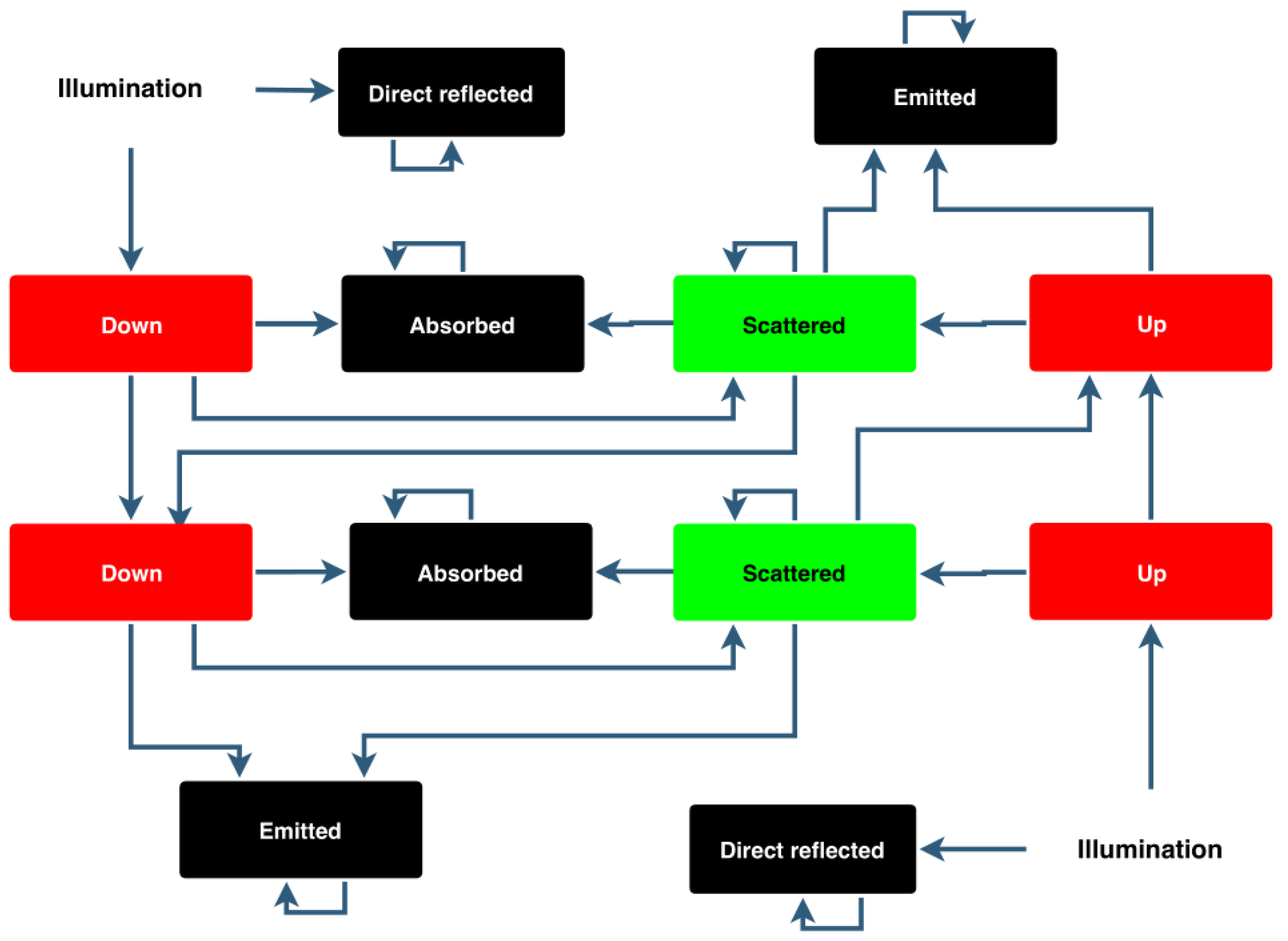
SLOP is a stochastic model of leaf optical properties based on Markov chains. It was first introduced by Tucker and Garratt in 1977 [23] and improved by Maier et al. in 1999 [22]. It takes leaf properties (see

Table 1. Constants and variables used in making training, testing, and validation data with SLOP. The training, testing, and validation data consist of 500,000 spectra made with SLOP. Each spectrum is produced by taking a random value from each interval in the table and calculating SLOP for each specified wavelength. The spectra are divided into training, testing, and validation data randomly, with constant sizes.

		Leaf Layer
		Palisade	Spongy
Variables	Chlorophyll a concentration ($\mathrm{m}$$\mathrm{g}$/$\mathrm{c}{\mathrm{m}}^3$)	[1, 10]	[0, 4]
	Chlorophyll b concentration ($\mathrm{m}$$\mathrm{g}$/$\mathrm{c}{\mathrm{m}}^3$)	[0.5, 5.5]	[0, 3]
	$\beta$-carotene concentration ($\mathrm{m}$$\mathrm{g}$/$\mathrm{c}{\mathrm{m}}^3$)	[0, 1]	[0, 0.5]
	Lutein concentration ($\mathrm{m}$$\mathrm{g}$/$\mathrm{c}{\mathrm{m}}^3$)	[0, 1]	[0, 0.5]
	Violaxanthin concentration ($\mathrm{m}$$\mathrm{g}$/$\mathrm{c}{\mathrm{m}}^3$)	[0, 0.5]	[0, 0.25]
	Neoxanthin concentration ($\mathrm{m}$$\mathrm{g}$/$\mathrm{c}{\mathrm{m}}^3$)	[0, 0.5]	[0, 0.25]
	Water content ($\mathrm{c}{\mathrm{m}}^3$/$\mathrm{c}{\mathrm{m}}^3$)	[0.8, 1]	[0.1, 0.5]
	scattering coefficient (1/$\mathrm{c}$$\mathrm{m}$)	[3.5, 5.5]	[1000, 1100]
	Probability of direct reflection	[0.4, 0.06]
Constants	Chloroplast diameter ($\mathrm{c}\mathrm{m}$)	0.0005
	Chloroplast concentration (1/$\mathrm{c}$${\mathrm{m}}^3$)	$5\times {10}^{-9}$	$6.7\times {10}^{-8}$
	Thickness ($\mathrm{c}\mathrm{m}$)	0.0069	0.0069

) and wavelength as an input and calculates leaf reflectance, transmittance, and absorbance. The basic idea of the stochastic modeling approach is that the leaf is modeled as a network of different states and their connections. For each connection, there is a corresponding probability for transition between states. The possible transitions in a leaf are described in Figure 1. The black boxes are end states where the only possible transition is to itself. In each layer of the leaf (see Figure 1) the photon goes to the next layer (or out), goes to the previous layer (or out) due to scattering, or it is absorbed into the layer. Each of these can also happen after scattering and therefore each layer contains four basic states: down, up, absorbed, and scattered. In addition, there are two white illumination states—for input—and four end states on the outside of the leaf. For each of these events probabilities are calculated based on the layer structure and pigment concentrations with the help of Beer’s law. For each transition, the probability is calculated as follows:

• For each up (similarly down) state, the up (down), scattering and absorption probabilities are

  $$\begin{array}{cc}\hfill P_{\mathrm{absorption}}\left(\lambda \right)& =\frac{a\left(\lambda \right)}{a\left(\lambda \right)+s}·(1-e^{-\left(a\right(\lambda )+s)·L}),\hfill \end{array}$$

  (1)

  $$\begin{array}{cc}\hfill P_{\mathrm{scattering}}\left(\lambda \right)& =\frac{s}{a\left(\lambda \right)+s}·(1-e^{-\left(a\right(\lambda )+s)·L}),\hfill \end{array}$$

  (2)

  $$\begin{array}{cc}\hfill P_{\mathrm{up} \left(\mathrm{down}\right)}\left(\lambda \right)& =1-P_{\mathrm{absorption}}-P_{\mathrm{scattering}}.\hfill \end{array}$$

  (3)
• For each scattered state the scattering and absorption probabilities are same as for the up and down states on the same layer. The up and down probabilities are

  $$P_{\mathrm{down}}\left(\lambda \right)=P_{\mathrm{up}}\left(\lambda \right)=\frac{1-P_{\mathrm{absorption}}-P_{\mathrm{scattering}}}{2}.$$

  (4)
• The probability of direct reflection is given as a parameter and the probability of entering the first layer is $1-P_{\mathrm{direct} \mathrm{reflection}}.$
• The probability of going from absorbed state, reflected state, or emitted state to itself is 1.
• All other transition probabilities are 0.

In the previous equations,

• $a\left(\lambda \right)$ is the absorption coefficient,

  $$a\left(\lambda \right)=\frac{\pi }{4}·(1+\frac{2e^{-\rho \left(\lambda \right)}}{\rho \left(\lambda \right)}+\frac{2(e^{-\rho \left(\lambda \right)}-1)}{\rho {\left(\lambda \right)}^2})·d_{\mathrm{chloroplast}}^2·c_{\mathrm{chloroplast}}+a_{H_{2}O}\left(\lambda \right)·w_{H_{2}O},$$

  (5)

  where

  $$\rho \left(\lambda \right)=\frac{6}{\pi }·\frac{1}{d_{\mathrm{chloroplast}}^2·c_{\mathrm{chloroplast}}}\sum _{\mathrm{pigments}}{a}_i·c_i,$$

  (6)
• s is the scattering coefficient,
• L is the length of the light path, which is assumed to be the same as the thickness of the layer,
• $a_i$ are the absorption coefficients of the pigments (chlorophyll a, chlorophyll b, beta-carotene, lutein, violaxanthin, neoxanthin) [22,25,26,27,28,29] and
• $c_i$ are their concentrations,
• $a_{H_{2}O}$ and $w_{H_{2}O}$ are the absorption coefficient [30,31,32] and volume concentration ($\mathrm{c}{\mathrm{m}}^3$/$\mathrm{c}{\mathrm{m}}^3$) of liquid water, and
• $d_{\mathrm{chloroplast}}$ is the diameter of chloroplast ($\mathrm{c}\mathrm{m}$) and $c_{\mathrm{chloroplast}}$ is its concentration (1/$\mathrm{c}{\mathrm{m}}^3$).

Table 1 shows the inputs and constants SLOP uses to calculate the previously introduced probabilities.

Mathematically, the Markov chain is handled as a matrix multiplication routine. The algorithm is the following:

• Initialize the state vector: The initial state of the network of states, for example “all photons coming from above, none inside” corresponds to the following state vector:

  $${\left[\begin{array}{c}{x}_0\\ x_1\\ x_2\\ ⋮\\ x_k\end{array}\right]}_0=\left[\begin{array}{c}1\\ 0\\ 0\\ ⋮\\ 0\end{array}\right]$$
• Matrix multiplication: The new state vector is the transition probability matrix multiplied with the old state vector:

  $${\left[\begin{array}{c}{x}_0\\ x_1\\ x_2\\ ⋮\\ x_k\end{array}\right]}_{n+1}=\left[\begin{array}{cccc}{P}_{0,0}& P_{0,1}& \cdots & P_{0,k}\\ ⋮& ⋮& \cdots & ⋮\\ P_{k,0}& P_{k,1}& \cdots & P_{k,k}\end{array}\right]{\left[\begin{array}{c}{x}_0\\ x_1\\ x_2\\ ⋮\\ x_k\end{array}\right]}_n$$
• Check the end condition: If the new and old state vectors are close enough to each other, end; otherwise, repeat from step 2. If

  $$\left|{\left[\begin{array}{c}{x}_0\\ x_1\\ x_2\\ ⋮\\ x_k\end{array}\right]}_{n+1}-{\left[\begin{array}{c}{x}_0\\ x_1\\ x_2\\ ⋮\\ x_k\end{array}\right]}_n\right|<ϵ,$$

  then each $x_i$ in the final state vector corresponds to the probability that the photon will end up in that state.

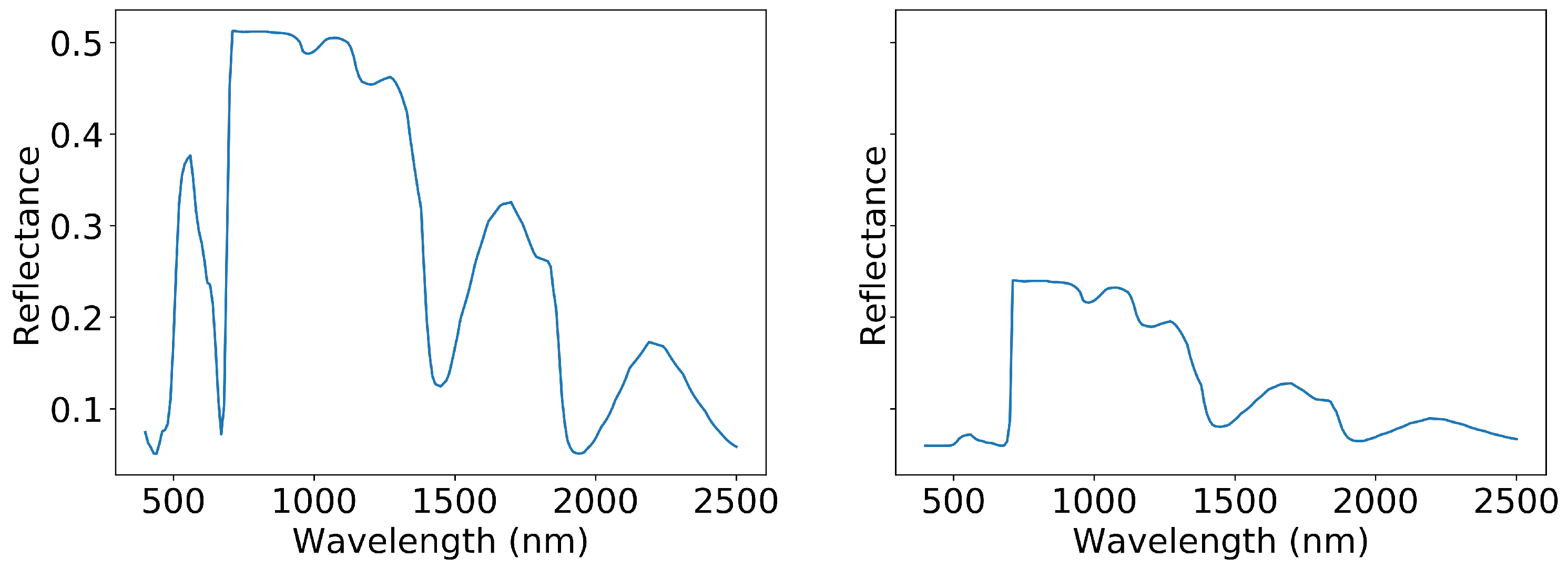
In this research, SLOP was used in making training, testing, and validation datasets for 1DCNN training. The input wavelengths depended on the validation scheme. With simulated validation data wavelengths from 400 $\mathrm{n}$$\mathrm{m}$ to 2500 $\mathrm{n}$$\mathrm{m}$ with 10 $\mathrm{n}$$\mathrm{m}$ spacing were used and with empirical validation data the first 19 wavelengths from

Table 2. Wavelength and full width of the half maximum (FWHM) values of the measured hyperspectral data [41].

Wavelength (nm):	507.60, 509.50, 514.50, 520.80, 529.00, 537.40, 545.80, 554.40, 562.70, 574.20, 583.60, 590.40, 598.80, 605.70, 617.50, 630.70, 644.20, 657.20, 670.10, 677.80, 691.10, 698.40, 705.30, 711.10, 717.90, 731.30, 738.50, 751.50, 763.70, 778.50, 794.00, 806.30, 819.70
FWHM (nm):	11.2, 13.6, 19.4, 21.8, 22.6, 20.7, 22.0, 22.2, 22.1, 21.6, 18.0, 19.8, 22.7, 27.8, 29.3, 29.9, 26.9, 30.3, 28.5, 27.8, 30.7, 28.3, 25.4, 26.6, 27.5, 28.2, 27.4, 27.5, 30.5, 29.5, 25.9, 27.3, 29.9

were used. The other inputs for SLOP are described in Table 1. Example spectra produced with SLOP can be seen in Figure 2.

2.2. Convolutional Neural Network

Convolutional neural networks (CNN) were first introduced by LeCun and Bengio in 1995 [13]. Traditional dense neural networks with hidden layers are based on matrix multiplication [33], where a convolutional layer replaces multiplication with convolution. CNNs are considered especially powerful for image-related tasks, such as image classification [8,9], or regression problems concerning images, such as object detection [10]. Altogether, CNN has been found to work well with signals [11,12].

The used 1DCNN architecture is described in

Table 3. The architecture of the used one-dimensional convolutional neural network (1DCNN).

Layer	Kernel/Pool Size and Activation	Filters/Units
Batch Normalization
Conv1D	3 ReLU	64
Batch Normalization
MaxPooling1D	3
Conv1D	3 ReLU	128
Batch Normalization
Dropout (0.15)
Flatten
Dense	ReLU	100
Dense	ReLU	1
Optimiser:	Adam
Loss:	Mean square error
Accuracy:	$r^2$-score

. It consisted of 1D convolution with 64 filters and a kernel size of 3, 1D pooling with a kernel size of 3, another 1D convolution with a kernel size of 3 and 128 filters, 15% dropout, a 100-filter dense layer and a dense output layer, and batch normalization [34] at the beginning and after each convolution layer. Input shape, and therefore the shape of each layer, depended on the shape of the training data. In this study, two different input data shapes were used. For the simulated validation data, the input data had a length of 210 and in the case of remotely sensed validation data it had a length of 19. Each layer that had an activation function used rectified linear unit activation [35]. The Adam optimizer was used [36], with a learning rate of $0.001$, ${\beta }_1=0.9$, ${\beta }_2=0.999$, and $ϵ={10}^{-7}$. The loss score was mean square error (MSE) [37], and the accuracy score was the coefficient of determination or, as it is also called, the $r^2$-score [38]. The dropout layers and batch normalization were added to reduce overfitting and also to help transition from the simulated data to the noisy empirical data.

All neural network implementation was performed with a Keras [39] package using the TensorFlow [40] backend. The computer used in neural network training had an Nvidia GT1080 16 Gb GPU.

Training data for the 1DCNN was split from the dataset produced by SLOP. For simulated data validation these data were used as they were, and for the case with remotely sensed data some Gaussian noise (M = 0, SD = 0.025) was added to the data. In both cases chlorophyll a and b estimators were trained separately.

2.3. Empirical Dataset

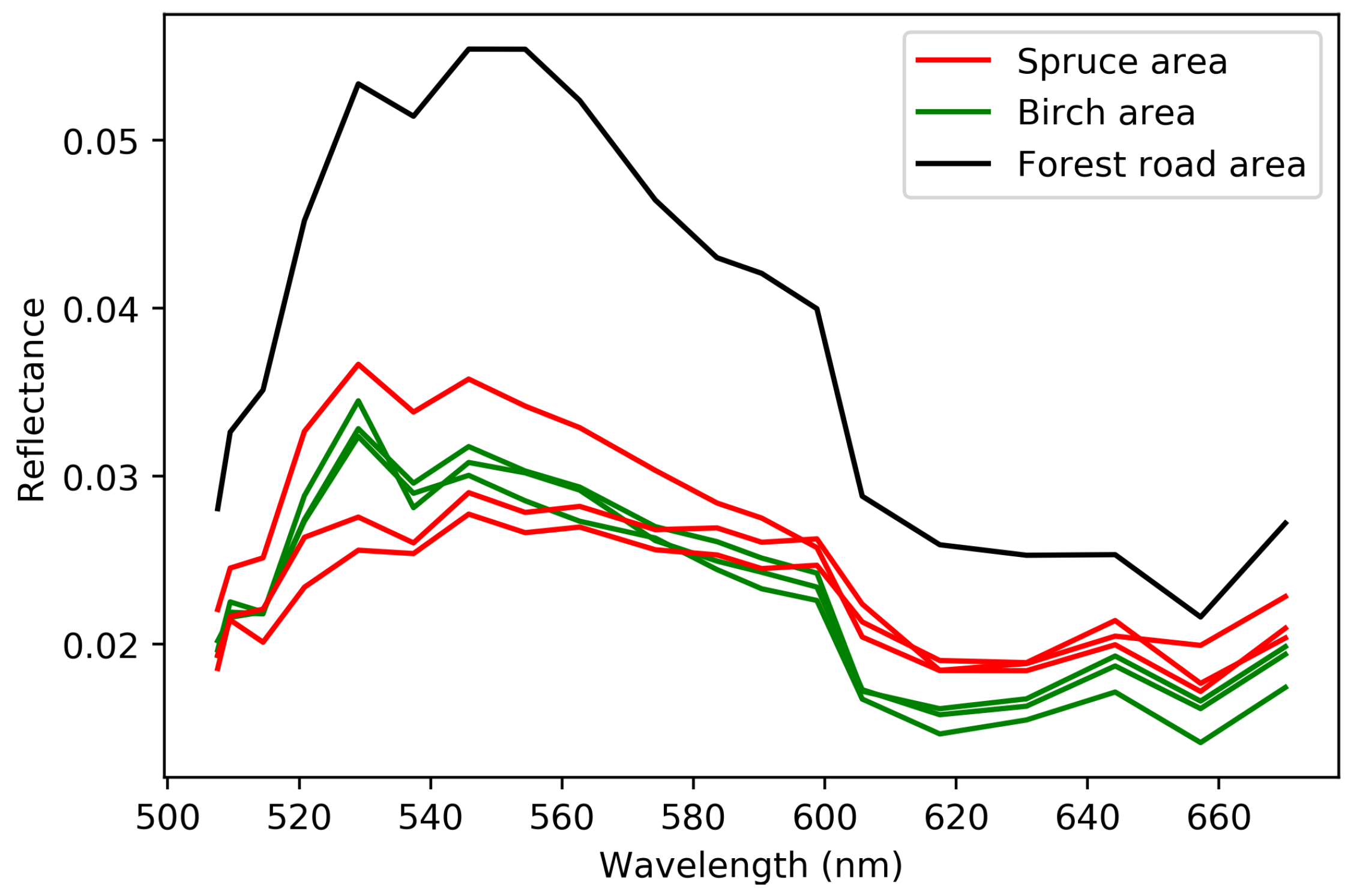
The empirical test site was located in the Vesijako experimental forest area in the municipality of Padasjoki in southern Finland. The test site was covered by young to middle-aged forest dominated by birch (Betula pendula), with spruce (Picea abies) as a secondary tree species. The flight campaign was carried out on 26 June 2014 from 12:09 to 12:22 using a hexacopter UAV. The weather conditions were cloudy. The hyperspectral images were captured using a 2D frame format hyperspectral camera based on a tunable Fabry–Pérot interferometer (FPI). The flying height was 88 $\mathrm{m}$ from the ground level, providing an average ground sampling distance (GSD) of $8.8$ $\mathrm{c}$$\mathrm{m}$ for the FPI images at ground level; the flight height was 67 $\mathrm{m}$ from the tree treetops, giving a GSD of $6.7$ $\mathrm{c}$$\mathrm{m}$ at the treetops. Hyperspectral orthophoto mosaics were calculated with a 10 $\mathrm{c}$$\mathrm{m}$ GSD and calibrated to reflectance units using the Finnish Geospatial Research Institute’s (FGI) in-house mosaicking software. The wavelengths measured were from $507.6$ $\mathrm{n}$$\mathrm{m}$ to $885.6$ $\mathrm{n}$$\mathrm{m}$, of which only 19 wavelength bands up to 671 $\mathrm{n}$$\mathrm{m}$ were used for neural network training and validation. All wavelengths were available for index calculations. Table 2 presents wavelength and full width of the half maximum (FWHM) values in detail. Example spectra can be seen in Figure 3. For details of the datasets and post-processing, see Nevalainen et al. [41]

2.4. Validation

The results of the neural network training were validated in two different ways. The first corresponds to an ideal scenario: The validation data are produced by SLOP and the assessment represents a case in which the measurements are noiseless and perfectly calibrated. In the second scenario, the inversion model was validated with empirical hyperspectral UAV data from a boreal forest. The second scenario can be further divided into three subscenarios:

• Calculation of chlorophyll a and b maps and comparison with the $\frac{\mathrm{TCARI}}{\mathrm{OSAVI}}$ index (TCARI = transformed chlorophyll absorption reflectance index, OSAVI = optimized soil adjusted vegetation index), a spectral index that is known for having a strong negative correlation with chlorophyll concentration [42],
• Comparison of simulated and measured $\frac{\mathrm{TCARI}}{\mathrm{OSAVI}}$ indices,
• Chlorophyll a/b ratio comparison to literature.

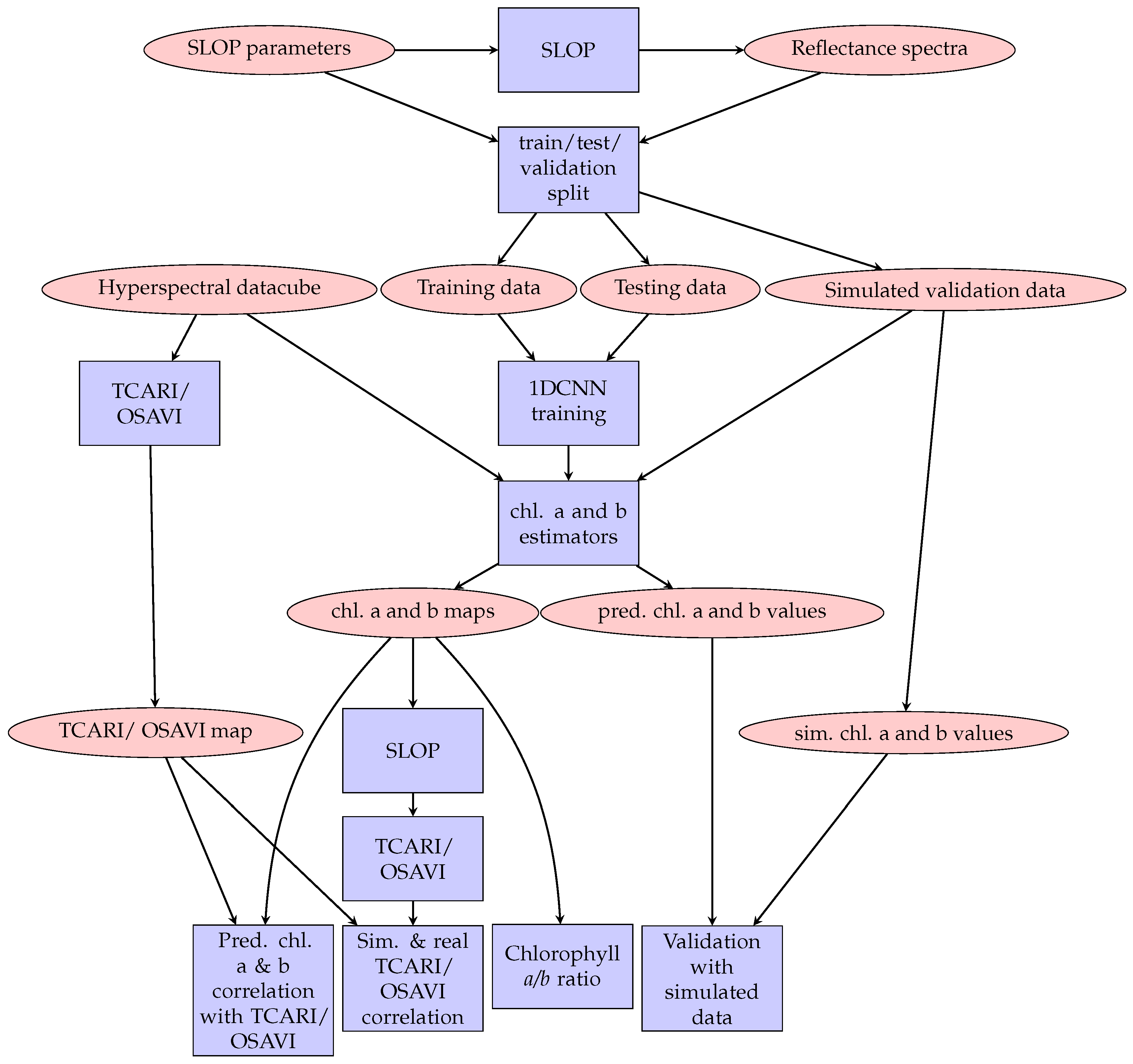
Figure 4 summarizes the proposed workflow and used methods.

Figure 3. Median spectrum from each plot 1–7 described in Figure 5.

Figure 3. Median spectrum from each plot 1–7 described in Figure 5.

2.4.1. Simulated Validation Dataset

In order to validate the method, the simulated data was divided into the training (45%), testing (22%), and validation (33%) datasets. The estimator was trained with the training and testing data and validated with the independent validation dataset. The predicted concentrations were provided by the estimator and compared to the validation data. Then the following metrics for the original and predicted concentrations were calculated:

• $r^2$ score between predicted and original values,
• Correlation coefficient between original and predicted values,
• MSE of their difference,
• Average difference,
• Standard deviation for the difference, and
• 95% confidence interval for the difference.

2.4.2. Empirical Validation Dataset

With the remotely sensed validation data, chlorophyll a and b maps were calculated by using the empirical data as input into the trained estimators. First, however, the data was shifted with a linear shift of 0.02 in order to get it to the same level as the training data and to eliminate negative values, that remained in the data after calibration. Since chlorophyll measurements for the data were not available, one had to acquire the concentrations using an alternative approach. Therefore, chlorophyll a and b predictions were compared to the $\frac{\mathrm{TCARI}}{\mathrm{OSAVI}}$ index. TCARI and OSAVI are calculated as follows:

$$\mathrm{TCARI}=3·(\mathrm{sel}(700 \mathrm{n}\mathrm{m})-\mathrm{sel}(670 \mathrm{n}\mathrm{m}))-0.2·(\mathrm{sel}(700 \mathrm{n}\mathrm{m})-\mathrm{sel}(500 \mathrm{n}\mathrm{m}))·\frac{\mathrm{sel}(700 \mathrm{n}\mathrm{m})}{\mathrm{sel}(670 \mathrm{n}\mathrm{m})}$$

(7)

and

$$\mathrm{OSAVI}=(1+0.16)·\frac{\mathrm{sel}\left(800 \mathrm{n}\mathrm{m}\right)-\mathrm{sel}\left(670 \mathrm{n}\mathrm{m}\right)}{\mathrm{sel}\left(800 \mathrm{n}\mathrm{m}\right)+\mathrm{sel}\left(670 \mathrm{n}\mathrm{m}\right)+0.16}$$

(8)

where the function sel chooses the wavelength band nearest to the desired band from the dataset. In this case, these were

$$\begin{array}{cc}\hfill \mathrm{sel}\left(700 \mathrm{n}\mathrm{m}\right)& =698.40 \mathrm{n}\mathrm{m},\hfill \\ \hfill \mathrm{sel}\left(670 \mathrm{n}\mathrm{m}\right)& =670.10 \mathrm{n}\mathrm{m},\hfill \\ \hfill \mathrm{sel}\left(500 \mathrm{n}\mathrm{m}\right)& =507.60 \mathrm{n}\mathrm{m},\hfill \\ \hfill \mathrm{sel}\left(800 \mathrm{n}\mathrm{m}\right)& =794.00 \mathrm{n}\mathrm{m}.\hfill \end{array}$$

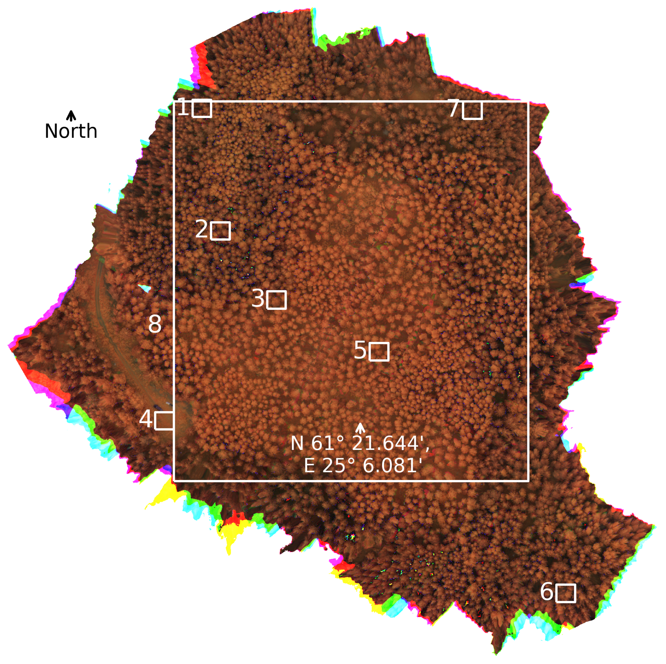
After calculating the different maps, each map was smoothed with a sliding $8\times 8$ pixel averaging window to account for camera noise. The maps were compared with each other on a large scale and in more detail using the plots described in Figure 5. The plots were selected so that they represent the forest area well. In the middle of it, there is an area that is mainly birch forest, and the border areas are spruce dominated. There is also a forest road. Three plots were chosen from the spruce-dominated area (plots 1, 6, and 7), two in the birch-dominated area (plots 2, 3, and 5), and one from the forest road (plot 4). Plot 8 is a larger plot combining large areas of both spruce- and birch-dominated parts of the forest.

2.4.3. Comparison of Simulated and Measured $\frac{\mathrm{TCARI}}{\mathrm{OSAVI}}$ Indices

$\frac{\mathrm{TCARI}}{\mathrm{OSAVI}}$ index was calculated with simulated data in order to compare it to the measured $\frac{\mathrm{TCARI}}{\mathrm{OSAVI}}$ index calculated in the previous chapter. The estimated chlorophyll a and b values for plots 1–7 were used as inputs for SLOP, while other inputs were averages of the intervals in Table 1. With SLOP, the reflectances on wavelengths 500 $\mathrm{n}$$\mathrm{m}$, 670 $\mathrm{n}$$\mathrm{m}$, 700 $\mathrm{n}$$\mathrm{m}$, and 800 $\mathrm{n}$$\mathrm{m}$ were simulated and used to calculate the simulated $\frac{\mathrm{TCARI}}{\mathrm{OSAVI}}$ for plots 1–7. Then they were compared visually and the correlations between them and the empirical $\frac{\mathrm{TCARI}}{\mathrm{OSAVI}}$ were calculated. The simulated map was limited to between 2 and 98 percentiles in order to remove the outliers in the simulated data.

2.4.4. Chlorophyll a/b

The chlorophyll a/b ratio map was also compared to common values for birch and spruce chlorophyll ratio. The birch chlorophyll ratios during early summer found in the literature were between 2.3 [43] and 3.78 [44]. For spruce, the corresponding interval was from 1.47 [45] to 3.75 [46].

3. Results and Discussion

3.1. Simulated Validation Dataset

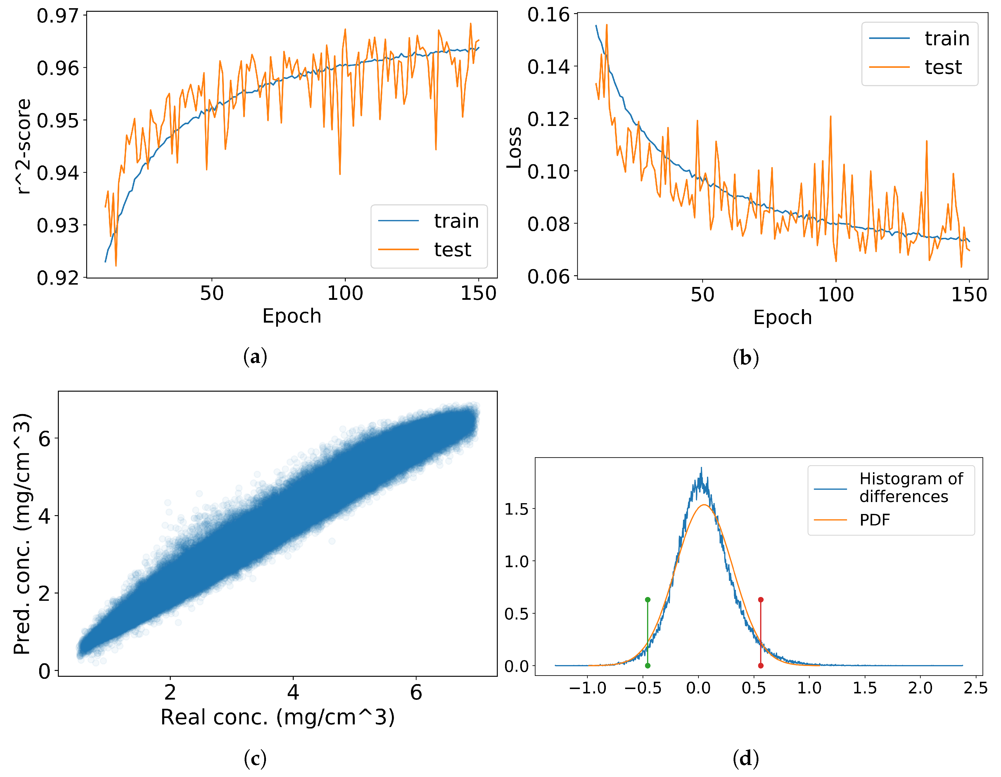
The MSE and $r^2$ scores converged during the training of the 1DCNN to 0 and 1 respectively and neither graph showed signs of over- or under-fitting (Figure 6), which holds for both the chlorophyll a and b training.

For the simulated validation dataset, the $r^2$ score between the original and predicted values was 0.97 for chlorophyll a and 0.95 for chlorophyll b. The correlation coefficient was 0.98 between the predicted and original chlorophyll a concentrations and 0.98 between the predicted and original chlorophyll b concentrations. The MSE was 0.07 between the original and predicted chlorophyll a values and 0.03 for the original and predicted chlorophyll b concentrations. The average difference in chlorophyll a predictions compared to original values was 0.05, with a standard deviation of 0.26. Thus, the difference between predicted and original values was between −0.46 and 0.56 with 95% probability. For chlorophyll b the corresponding values were the following: mean 0.02, standard deviation 0.18, 95% confidence interval $[-0.34,0.37]$ (Figure 6c,d,g,h and

Table 4. Results of training and validating the CNN estimators for chlorophyll a and b.

	Chlorophyll a	Chlorophyll b
$r^2$ score between original and predicted values	0.97	0.95
Correlation coefficient between original and predicted values	0.98	0.98
MSE	0.07	0.03
Average difference	0.05	0.02
Standard deviation	0.26	0.18
95% Confidence interval of the difference between predicted and original values	$[-0.46,0.56]$	$[-0.34,0.37]$

).

The results indicate that the estimators predict simulated chlorophyll a and b values accurately. This means that if the SLOP model is assumed to be perfect, the used hyperspectral camera is optimal with a spectral range of 400 $\mathrm{n}$$\mathrm{m}$ to 2600 $\mathrm{n}$$\mathrm{m}$ and illumination conditions are perfect, the chlorophyll a and b estimators give reasonably accurate results. Compared to previous research, the used network matched the results received in the past. Croft et al. simulated spectral data from multiple sensors and obtained $r^2$ scores of 0.96–0.99 when they compared their results to chlorophyll concentrations [14].

3.2. Empirical Validation Dataset

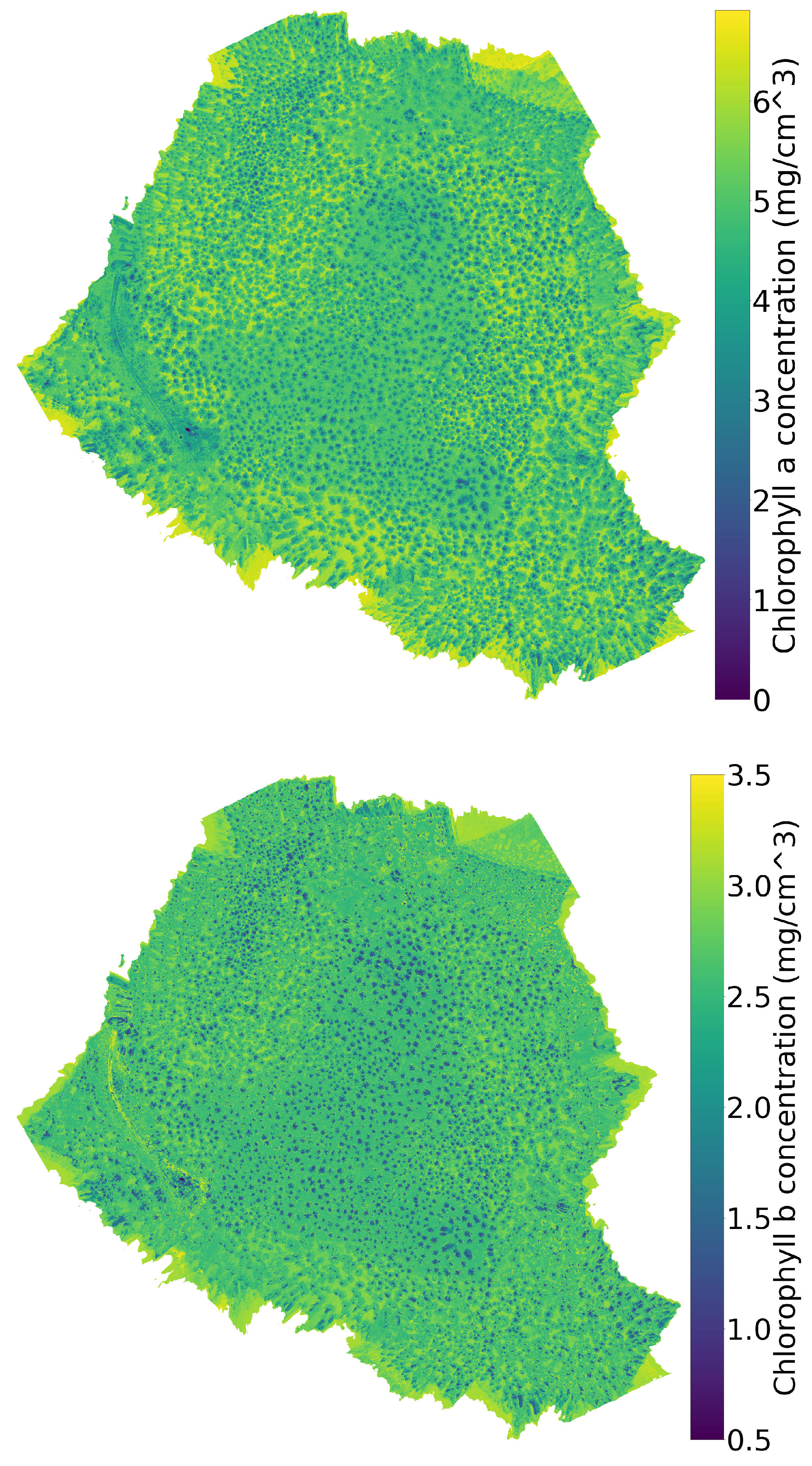
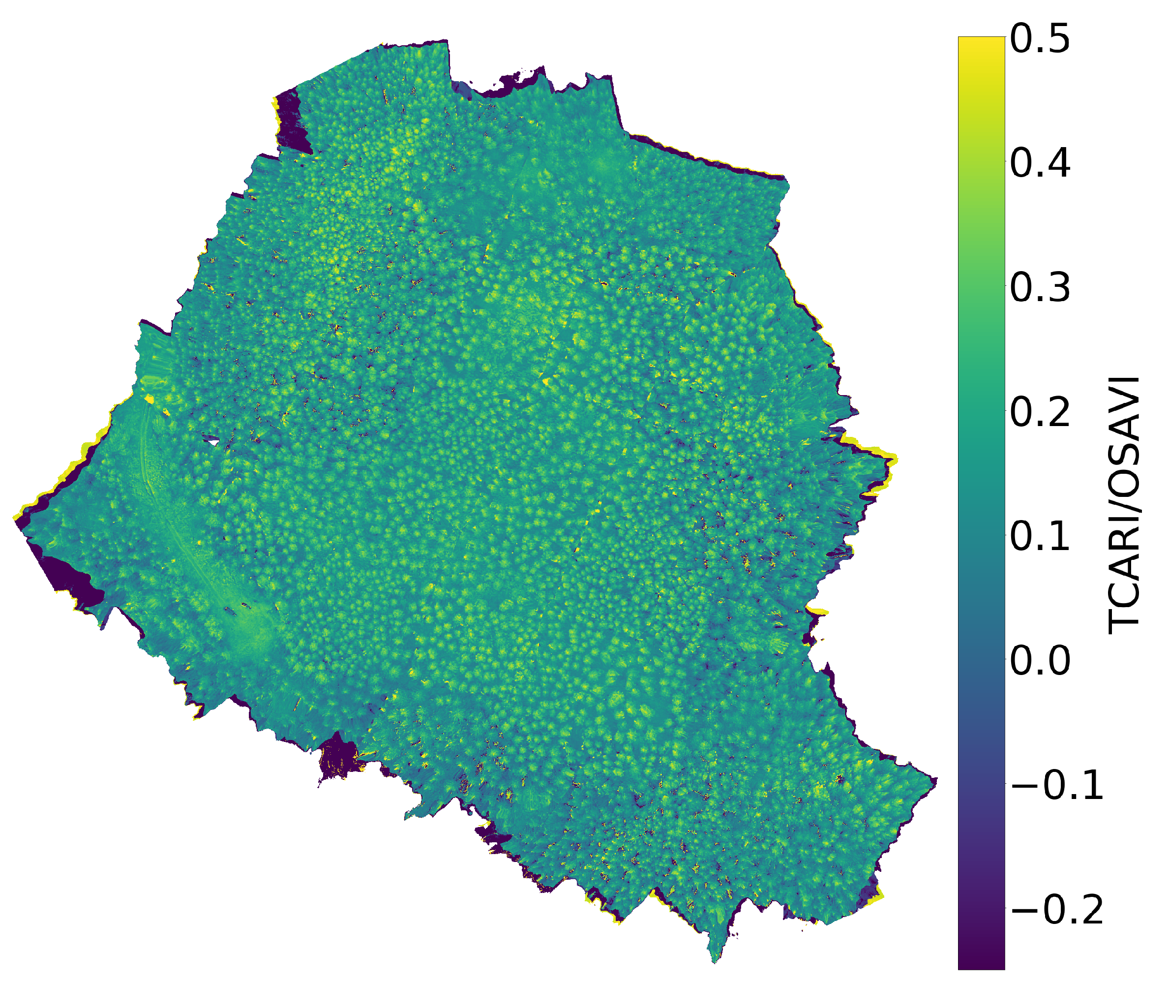
The results involving measured hyperspectral validation data can be seen in Figure 7, Figure 8, Figure 9, Figure 10, Figure 11 and

Table 5. Correlation coefficients between predicted chlorophyll values and the $\frac{\mathrm{TCARI}}{\mathrm{OSAVI}}$ index in the eight researched plots.

	Correlation Coefficient for Chlorophyll a and Index	Correlation Coefficient for Chlorophyll b and Index	Plot Description
Plot 1	−0.91	−0.81	Spruce
Plot 2	−0.90	−0.83	Birch
Plot 3	−0.84	−0.61	Birch
Plot 4	−0.81	−0.61	Forest road
Plot 5	−0.93	−0.88	Birch
Plot 6	−0.91	−0.74	Spruce
Plot 7	−0.88	−0.55	Spruce
Plots 1, 6 and 7	−0.90	−0.70	Spruce
Plots 2, 3 and 5	−0.89	−0.77	Birch
Plots 1–7	−0.87	−0.68	Spruce and Birch
Plot 8	−0.82	−0.76	Larger plot. Mainly birch, spruce on the border areas

and

Table 6. Correlation coefficients between simulated and empirical $\frac{\mathrm{TCARI}}{\mathrm{OSAVI}}$ indexes in the seven investigated plots.

	Correlation Coefficient between Simulated and Empirical $\frac{\mathbf{TCARI}}{\mathbf{OSAVI}}$ Indexes	Plot Description
Plot 1	0.89	Spruce
Plot 2	0.83	Birch
Plot 3	0.75	Birch
Plot 4	0.68	Forest road
Plot 5	0.88	Birch
Plot 6	0.85	Spruce
Plot 7	0.81	Spruce

. The chlorophyll a and b and $\frac{\mathrm{TCARI}}{\mathrm{OSAVI}}$ maps clearly resembled each other, with the birch and spruce areas distinguishable along with the forest road (Figure 7).

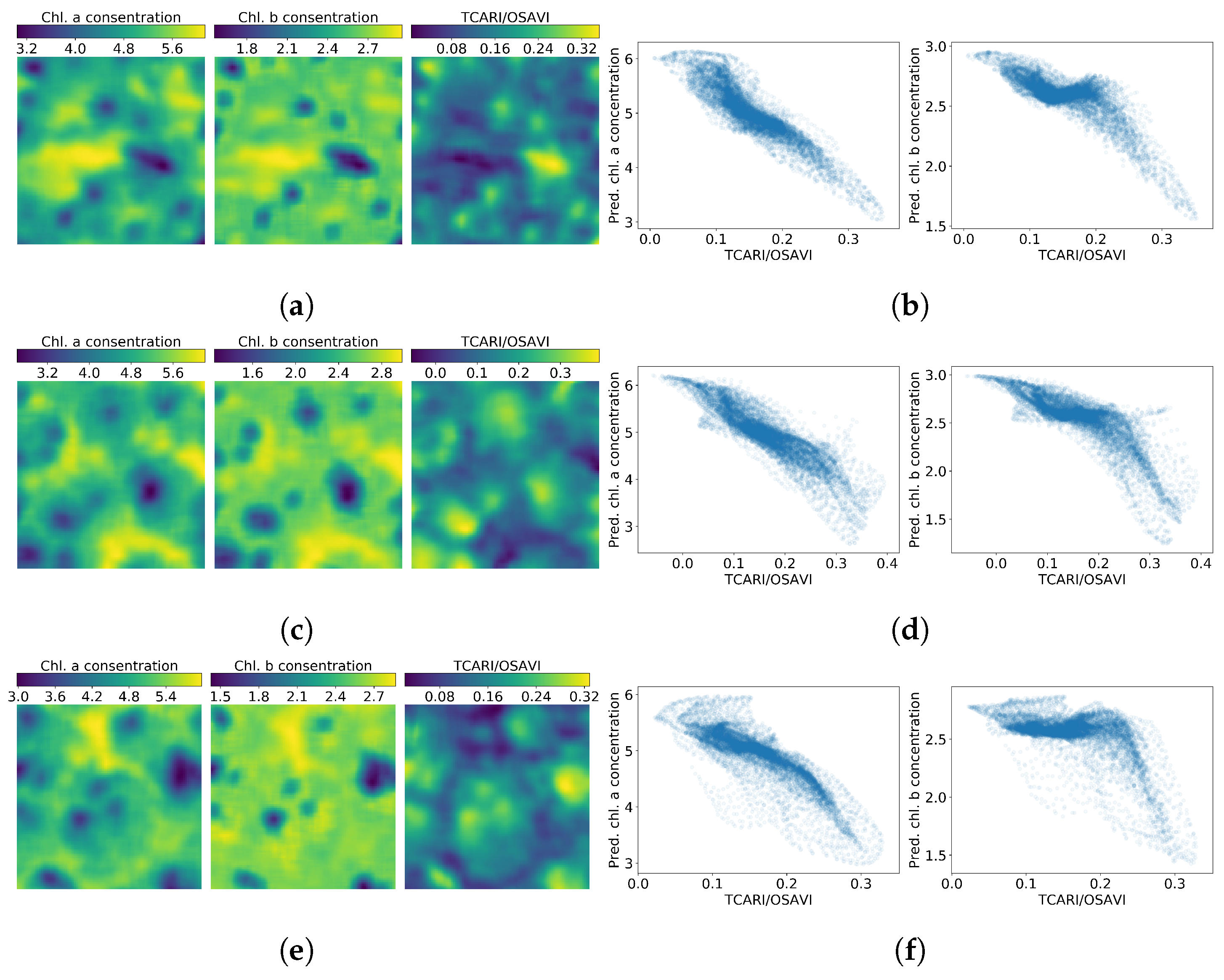
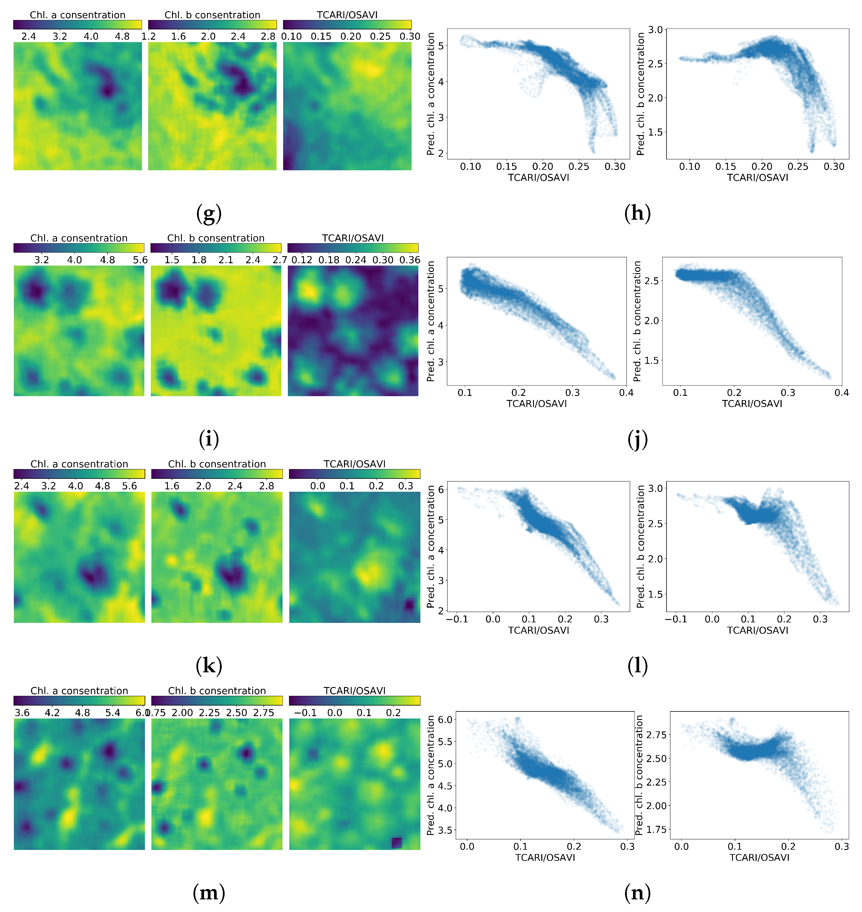
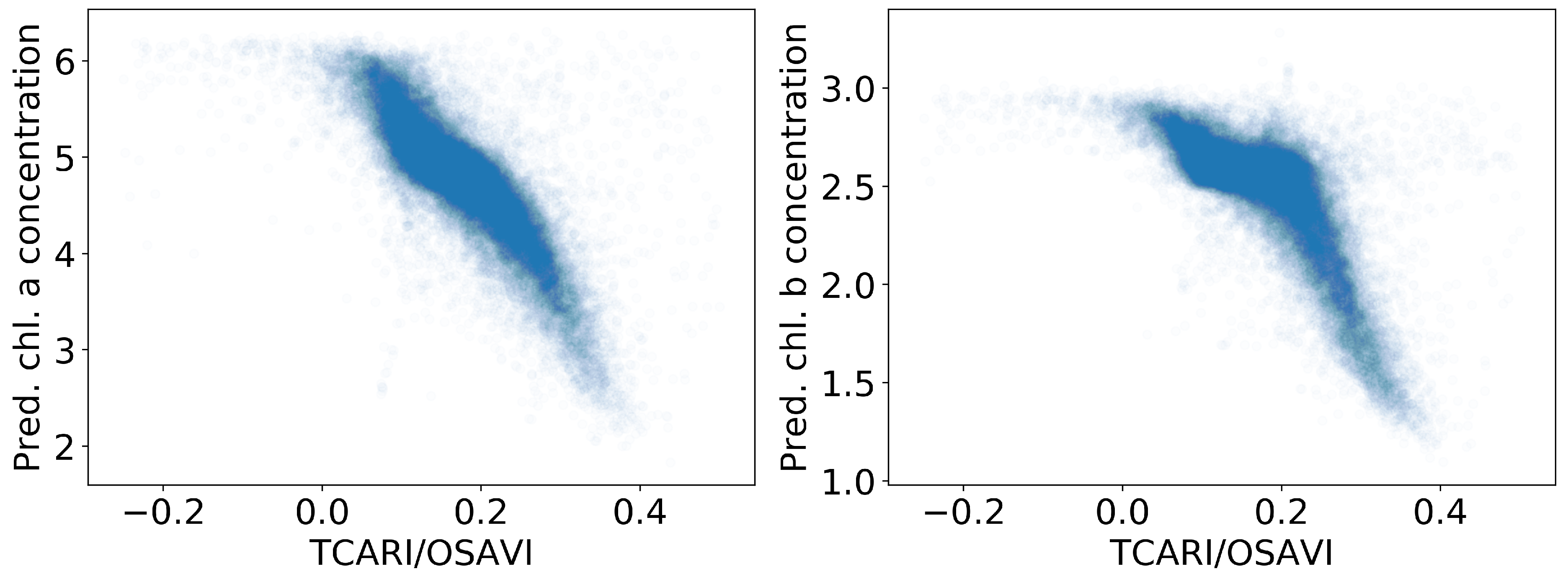
The predicted chlorophyll a and b correlated with the empirical $\frac{\mathrm{TCARI}}{\mathrm{OSAVI}}$ in the plots 1–7 described in Figure 5. In the spruce-dominant plots, the correlation coefficient was, on average, $-0.9$ for chlorophyll a and $-0.7$ for chlorophyll b. In the birch-dominated plots, the corresponding average correlation coefficients were $-0.89$ and $-0.77$ while in all of the plots 1–7 they were $-0.87$ and $-0.68$. The results for the plot 8 were $-0.82$ for chlorophyll a and $-0.76$ for chlorophyll b (Figure 8 and Figure 9 and Table 5).

We did not have reference data to assess the absolute accuracies, but results in Figure 7, Figure 8, and Figure 11 proposed that the results were at least proportionally correct. The estimated chlorophyll values of different land cover classes were consistent with the expectations (Figure 7). For example, the birch dominated area in the center of the forest was clearly separable from the spruce dominated area at the area perimeters, and the forest road obtained low chlorophyll values. As expected, the chlorophyll values were high for the low $\frac{\mathrm{TCARI}}{\mathrm{OSAVI}}$ values. Also, the analysis of the finer details indicated that these observations were correct (Figure 8). Comparisons of the values of predicted chlorophyll concentrations (Figure 7) to simulated values (Table 1) indicated that the values were of the same order of magnitude, which confirms that our approach could produce correct results if the training data has good quality.

While for chlorophyll a the relation with $\frac{\mathrm{TCARI}}{\mathrm{OSAVI}}$ was relatively linear, the corresponding connection for chlorophyll b had an approximately constant part when chlorophyll b was about $2.7$ $\mathrm{m}$$\mathrm{g}$/$\mathrm{c}{\mathrm{m}}^3$ and $\frac{\mathrm{TCARI}}{\mathrm{OSAVI}}$ increased from approximately $0.1$ to $0.2$ (Figure 8 and Figure 9). One possible reason is that the $\frac{\mathrm{TCARI}}{\mathrm{OSAVI}}$ correlation is with (combined) chlorophyll content, and its correlation with chlorophyll a and b separately has not been accounted for. In addition, chlorophyll a content is usually higher in plants, so it follows that chlorophyll b has a smaller net contribution in the correlation. To find the cause of the constant part, there is a need for further research and comparison of the inverse SLOP results to measured chlorophyll concentrations. If the constant part persists in such study, our postulation of the cause is false. At the moment we lack a proper dataset to conduct such research.

Our results are in line with previous research. Croft et al. found an $r^2$ score of 0.78 between modeled and measured chlorophyll concentrations, which assuming linearity would mean correlation similar to our results [14]. Results from [15] show an $r^2$ score of 0.87 between modeled and measured canopy chlorophyll content, which is slightly higher than what we obtained. The results are not directly comparable due to our lack of field chlorophyll measurements, and for a fair comparison of the results of this study, the method should be tested in further studies using in-situ chlorophyll measurements.

3.3. Comparison of Simulated and Measured $\frac{\mathit{TCARI}}{\mathit{OSAVI}}$ Indices

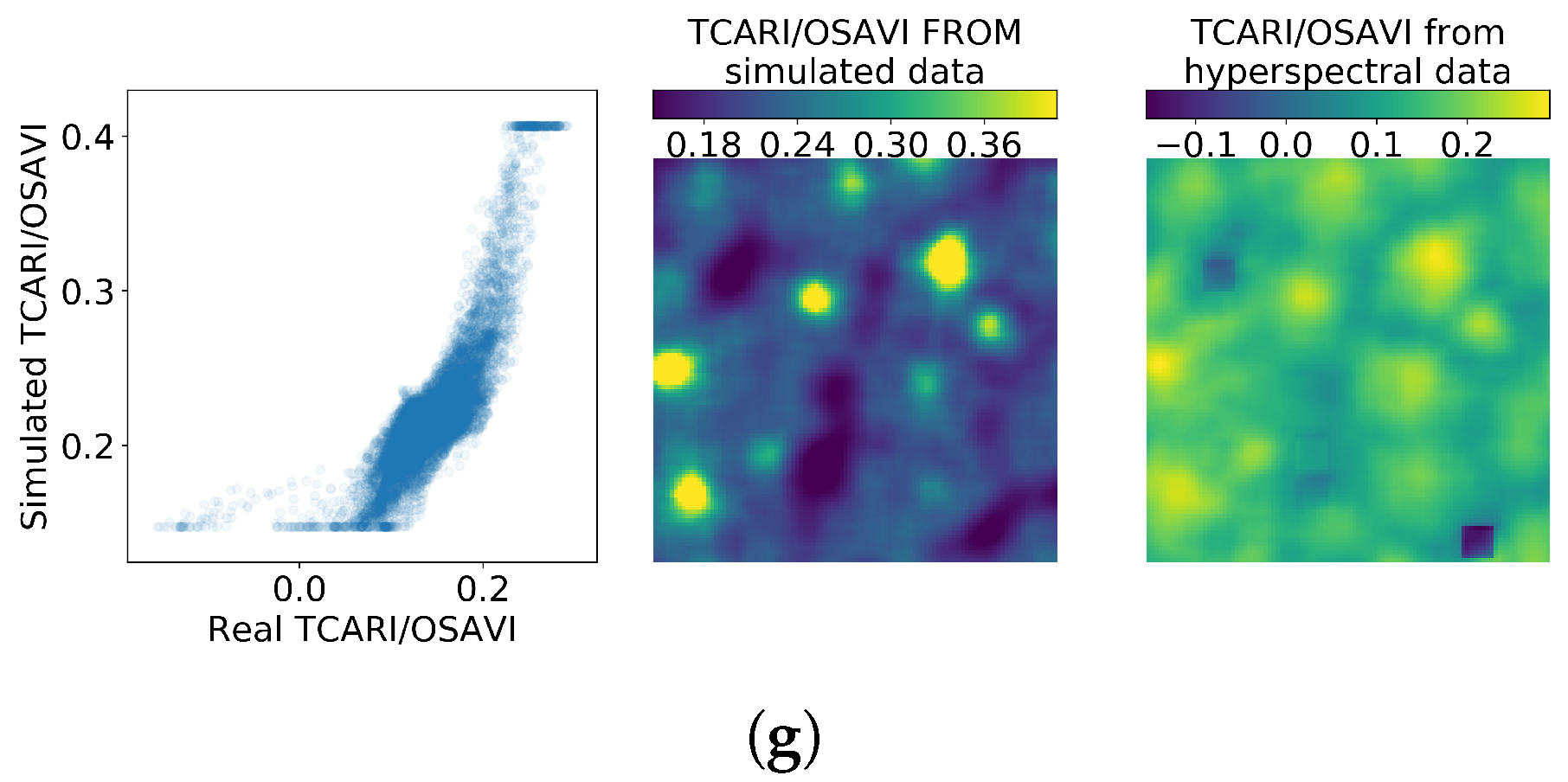
The simulated and empirical $\frac{\mathrm{TCARI}}{\mathrm{OSAVI}}$ indexes correlated strongly (see Figure 10 and Table 6). The correlation values ranged between 0.69 and 0.89, and the patterns were similar to each other and compared to Figure 8. This validates the SLOP model’s ability to produce data similar to empirical data and reinforces our conclusion that the 1DCNN estimators are truly emulating the true inverse function of SLOP in regards of chlorophyll a and b. If either of these conclusions were false, the data produced by SLOP would be significantly different from empirical data, and the error would propagate to the $\frac{\mathrm{TCARI}}{\mathrm{OSAVI}}$ calculation.

The reasoning of this assessment is the following. The $\frac{\mathrm{TCARI}}{\mathrm{OSAVI}}$ was calculated from the empirical validation data in two ways: by calculating directly from the empirical data and by using two different functions before calculating the $\frac{\mathrm{TCARI}}{\mathrm{OSAVI}}$. If the two approaches produced mutually correlating data, the two functions would act as approximate inverse function of each other. In addition, if the empirical validation data were vastly different from the data produced by SLOP, the trained inverse function would not have capability to explain the input and the output would be irrational.

3.4. Chlorophyll a/b

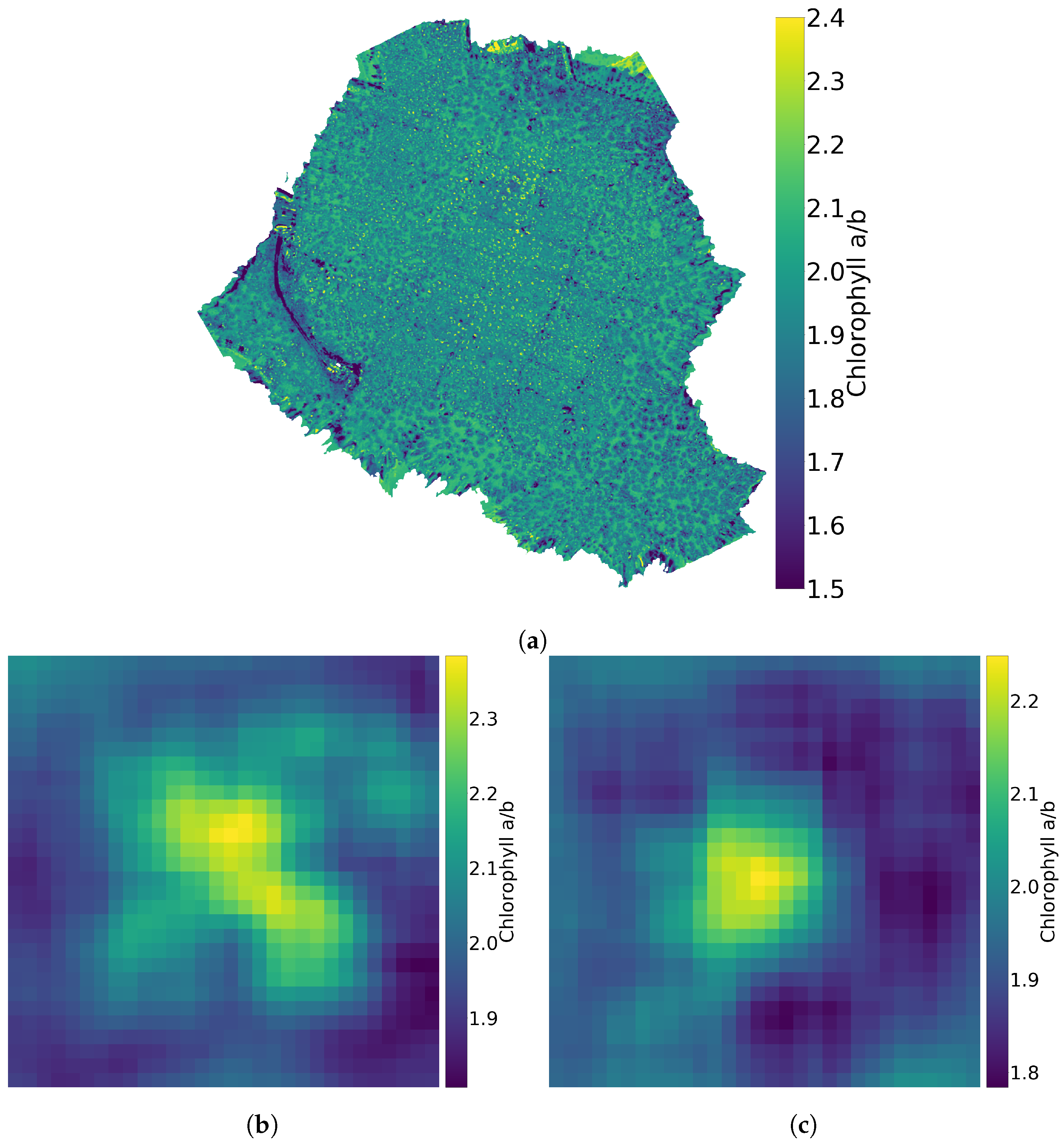
Chlorophyll a/b values ranged from 1.5 to 2.5 (see Figure 11) which was in line with spruce and birch intervals: from 1.47 to 3.75 for spruce [45,46] and from 2.3 to 3.78 for birch [43,44]. For spruce (Figure 11c) the values ranged from 1.8 to 2.2 and in the middle of the figure where the spruce stood the values were around 2.1 to 2.2, which were in the correct range. For the birch (Figure 11b) the values ranged from 1.85 to 2.35. In the middle the values were in between 2.1 and 2.35, which means that the values were at the lower end of the correct range.

3.5. Other Observations

The $\frac{\mathrm{TCARI}}{\mathrm{OSAVI}}$ index can also be used to estimate chlorophyll concentrations [42]. This estimation would be useful to correlate with our estimators, yet then the leaf area index (LAI) should be calculated. Unfortunately, it was not possible to estimate the LAI from the used empirical dataset.

In vegetation parameter retrieval studies, the leaf-level model is often paired to a canopy radiative transfer model (RTM) [14,15,17]. This procedure would have been advantageous in our study as well, and the fact that we used the leaf-level simulated spectral data instead of canopy-level features will cause some uncertainties in the analysis. However, we expect that these differences are smaller than in studies with conventional manned aircrafts or satellites. Firstly, our dataset had ultra-high spatial resolution with a ground sampling distance of 8 cm, thus spectral values of individual pixels had less mixing with background than the typical aircraft or satellite images with GSDs of e.g., 50 $\mathrm{c}$$\mathrm{m}$ to 10 $\mathrm{m}$. Secondly, the measurements took place in cloudy weather with diffuse illumination, thus the disturbing bidirectional reflectance (BRDF) effects were minimal in the data [41]. Thirdly, we added some Gaussian noise to the leaf-level training data, which could also account for some of the uncertainty that is introduced in transition from leaf-level to canopy-level. Even though we did not account for the canopy RTM, the results were consistent with the leaf level simulations. In future studies we will also implement the canopy RTM in our modeling. If the 1DCNN model is integrated with a radiative transfer simulator such as Librat [47], training data for various sensors and conditions could be generated.

Based on our literature review, the combination of using a simulation model for hyperspectral data and CNN for parameter retrieval is new in the field of hyperspectral data analysis. As discussed earlier, CNN is a powerful tool for signal regression and classification problems. It has been shown to perform better than traditional dense deep neural networks in image recognition and other signal-related tasks, thus it should perform better in regression problems concerning hyperspectral images. The use of simulated data in training is justified by the fact that obtaining a comprehensive dataset in field measurements requires a huge effort, whereas mathematical models can be developed with significantly less labor. Our approach of using simulated data for CNN training has the potential for a more universal and accurate regression and classification models in the context of hyperspectral imaging.

One of the difficult parts of using simulated data in parameter retrieval is accounting for error sources in hyperspectral images. The simulated data are smooth and noiseless, whereas the empirical data are vulnerable to multiple error sources. Two approaches to tackle this challenge are the development of rigorous data calibration approaches [4] and the implementation of different error sources to the canopy radiative transfer modeling [47]. In this study we attempted to take noise into account in the design of the CNN by adding batch Normalization layers to the bare-bones CNN template, by adding Gaussian noise to the training data and by averaging the resulting chlorophyll a and b and $\frac{\mathrm{TCARI}}{\mathrm{OSAVI}}$ maps over an $8\times 8$ pixel sliding window. There is still a need for development in this area to identify the best ways to control noise in hyperspectral images.

While it appears that our approach works relatively well with SLOP, it would be interesting to study different other models as well, such as ray tracing models [48,49], models specialized in coniferous trees [50], or models that take the entire forest stand into account [51,52,53,54]. They could improve the results, because SLOP is tied to the composition of the basic leaf. The ray tracing would be more accurate, but it would also require more computing time. In some cases, the use of a simpler or less accurate model could be justified if computation time is the limiting factor. It is also possible to obtain more specialized training data by narrowing the range of SLOP parameters around known values of some certain tree species. This would probably make results more accurate for that species while degrading the results for other tree species.

The 1DCNN model may not be the best possible network for the task. However, it has already shown promising results as the basis for the further developments. There is much work to do on developing CNN networks for different tasks, including regression and classification tasks in hyperspectral data analysis.

4. Conclusions

Our study has presented a novel method for chlorophyll a and b estimation from hyperspectral image data using the stochastic model of leaf optical (SLOP) properties and a convolutional neural network. We found that when the conditions and imaging system are consistent with the SLOP model, the convolutional neural network estimators for chlorophyll a and b produce feasible results. Our results showed that even with less-than-ideal remote sensing data, the results were in the right range and correlated well with an index known to correlate strongly with chlorophyll concentration. This indicates that our method shows promising results in measuring chlorophyll, although further verification of the results is needed to ensure their correctness.

We utilized a conventional one-dimensional convolutional neural network (CNN) structure, which showed promising performance. By optimizing the CNN model, the results are expected to improve, and the prediction errors are expected to decrease. The aim of further research could be developing a model based on CNN and hyperspectral data for reliable estimation of tree health through measurements of chlorophyll a and b.

References

1. Pan, Y.; Birdsey, R.A.; Fang, J.; Houghton, R.; Kauppi, P.E.; Kurz, W.A.; Phillips, O.L.; Shvidenko, A.; Lewis, S.L.; Canadell, J.G.; et al. A large and persistent carbon sink in the world’s forests. Science 2011, 333, 988–993. [Google Scholar] [CrossRef] [PubMed] [Green Version]
2. Rossini, M.; Panigada, C.; Meroni, M.; Colombo, R. Assessment of oak forest condition based on leaf biochemical variables and chlorophyll fluorescence. Tree Physiol. 2006, 26, 1487–1496. [Google Scholar] [CrossRef] [PubMed] [Green Version]
3. Bjorkman, C.; Niemela, P. Climate Change and Insect Pests; CABI: Wallingford, UK, 2015; Volume 8. [Google Scholar]
4. Aasen, H.; Honkavaara, E.; Lucieer, A.; Zarco-Tejada, P.J. Quantitative remote sensing at ultra-high resolution with UAV spectroscopy: A review of sensor technology, measurement procedures, and data correction workflows. Remote Sens. 2018, 10, 1091. [Google Scholar] [CrossRef] [Green Version]
5. Bioucas-Dias, J.M.; Plaza, A.; Camps-Valls, G.; Scheunders, P.; Nasrabadi, N.; Chanussot, J. Hyperspectral remote sensing data analysis and future challenges. IEEE Geosci. Remote Sens. Mag. 2013, 1, 6–36. [Google Scholar] [CrossRef] [Green Version]
6. Verrelst, J.; Camps-Valls, G.; Muñoz-Marí, J.; Rivera, J.P.; Veroustraete, F.; Clevers, J.G.; Moreno, J. Optical remote sensing and the retrieval of terrestrial vegetation bio-geophysical properties–a review. ISPRS J. Photogramm. Remote Sens. 2015, 108, 273–290. [Google Scholar] [CrossRef]
7. Verrelst, J.; Malenovskỳ, Z.; Van der Tol, C.; Camps-Valls, G.; Gastellu-Etchegorry, J.P.; Lewis, P.; North, P.; Moreno, J. Quantifying vegetation biophysical variables from imaging spectroscopy data: A review on retrieval methods. Surv. Geophys. 2018, 40, 589–629. [Google Scholar] [CrossRef] [Green Version]
8. Krizhevsky, A.; Sutskever, I.; Hinton, G.E. Imagenet classification with deep convolutional neural networks. In Proceedings of the Advances in Neural Information Processing Systems, Lake Tahoe, NV, USA, 3–8 December 2012; pp. 1097–1105. [Google Scholar]
9. Karpathy, A.; Toderici, G.; Shetty, S.; Leung, T.; Sukthankar, R.; Fei-Fei, L. Large-scale video classification with convolutional neural networks. In Proceedings of the IEEE conference on Computer Vision and Pattern Recognition, Columbus, OH, USA, 23–28 June 2014; pp. 1725–1732. [Google Scholar]
10. Szegedy, C.; Toshev, A.; Erhan, D. Deep neural networks for object detection. In Proceedings of the Advances in Neural Information Processing Systems, Lake Tahoe, NV, USA, 5–10 December 2013; pp. 2553–2561. [Google Scholar]
11. Cecotti, H.; Graeser, A. Convolutional neural network with embedded Fourier transform for EEG classification. In Proceedings of the 2008 19th International Conference on Pattern Recognition, Tampa, FL, USA, 8–11 December 2008; pp. 1–4. [Google Scholar]
12. Salamon, J.; Bello, J.P. Deep convolutional neural networks and data augmentation for environmental sound classification. IEEE Signal Process. Lett. 2017, 24, 279–283. [Google Scholar] [CrossRef]
13. LeCun, Y.; Bengio, Y. Convolutional networks for images, speech, and time-series. In The Handbook of Brain Theory and Neural Networks; MIT Press: Cambridge, MA, USA, 1995. [Google Scholar]
14. Croft, H.; Chen, J.; Zhang, Y.; Simic, A.; Noland, T.; Nesbitt, N.; Arabian, J. Evaluating leaf chlorophyll content prediction from multispectral remote sensing data within a physically-based modeling framework. ISPRS J. Photogramm. Remote Sens. 2015, 102, 85–95. [Google Scholar] [CrossRef]
15. Atzberger, C.; Jarmer, T.; Schlerf, M.; Kötz, B.; Werner, W. Retrieval of wheat bio-physical attributes from hyperspectral data and SAILH+ PROSPECT radiative transfer model. In Proceedings of the 3rd EARSeL Workshop on Imaging Spectroscopy, Herrsching, Germany, 13–16 May 2003; pp. 473–482. [Google Scholar]
16. Jacquemoud, S.; Baret, F. PROSPECT: A model of leaf optical properties spectra. Remote Sens. Environ. 1990, 34, 75–91. [Google Scholar] [CrossRef]
17. Jacquemoud, S.; Verhoef, W.; Baret, F.; Bacour, C.; Zarco-Tejada, P.J.; Asner, G.P.; François, C.; Ustin, S.L. PROSPECT+ SAIL models: A review of use for vegetation characterization. Remote Sens. Environ. 2009, 113, S56–S66. [Google Scholar] [CrossRef]
18. Tedesco, M.; Pulliainen, J.; Takala, M.; Hallikainen, M.; Pampaloni, P. Artificial neural network-based techniques for the retrieval of SWE and snow depth from SSM/I data. Remote Sens. Environ. 2004, 90, 76–85. [Google Scholar] [CrossRef]
19. Notarnicola, C.; Angiulli, M.; Posa, F. Soil moisture retrieval from remotely sensed data: Neural network approach versus Bayesian method. IEEE Trans. Geosci. Remote Sens. 2008, 46, 547–557. [Google Scholar] [CrossRef]
20. Trombetti, M.; Riaño, D.; Rubio, M.; Cheng, Y.; Ustin, S. Multi-temporal vegetation canopy water content retrieval and interpretation using artificial neural networks for the continental USA. Remote Sens. Environ. 2008, 112, 203–215. [Google Scholar] [CrossRef]
21. Cipollini, P.; Corsini, G.; Diani, M.; Grasso, R. Retrieval of sea water optically active parameters from hyperspectral data by means of generalized radial basis function neural networks. IEEE Trans. Geosci. Remote Sens. 2001, 39, 1508–1524. [Google Scholar] [CrossRef]
22. Maier, S.; Lüdeker, W.; Günther, K. SLOP: A Revised Version of the Stochastic Model for Leaf Optical Properties. Remote Sens. Environ. 1999, 68, 273–280. [Google Scholar] [CrossRef]
23. Tucker, C.; Garratt, M. Leaf optical system modeled as a stochastic process. Appl. Opt. 1977, 16, 635–642. [Google Scholar] [CrossRef]
24. Jacquemoud, S.; Ustin, L. Modeling leaf optical properties. Photobiol. Sci. Online 2008. Available online: http://photobiology.info/Jacq_Ustin.html (accessed on 10 January 2020).
25. Buschmann, C.; Nagel, E. Reflection Spectra Of Terrestrial Vegetation As Influenced By Pigment-protein Complexes And The Internal Optics Of The Leaf Tissue. In Proceedings of the Remote Sensing: Global Monitoring for Earth Management (IGARSS’91), Espoo, Finland, 3–6 June 1991; Volume 4, pp. 1909–1912. [Google Scholar] [CrossRef]
26. Lichtenthaler, H.K. [34] Chlorophylls and carotenoids: Pigments of photosynthetic biomembranes. In Plant Cell Membranes; Methods in Enzymology; Academic Press: Cambridge, MA, USA, 1987; Volume 148, pp. 350–382. [Google Scholar] [CrossRef]
27. Richter, T.; Fukshansky, L. Authentic in vivo absorption spectra for chlorophyll in leaves as derived from in situ and in vitro measurements. Photochem. Photobiol. 1994, 59, 237–247. [Google Scholar] [CrossRef]
28. Lichtenthaler, H.; Burkard, G.; Kuhn, G.; Prenzel, U. Light-Induced Accumulation and Stability of Chlorophylls and Chlorophyll-Proteins during Chloroplast Development in Radish Seedlings. Z. Naturforschung C 1981, 36, 421–430. [Google Scholar] [CrossRef] [Green Version]
29. Evans, J. A quantitative analysis of light distribution between the two photosystems, considering variation in both the relative amounts of the chlorophyll-protein complexes and the spectral quality of light. Photobiochem. Photobiophys. 1986, 10, 135–147. [Google Scholar]
30. Hale, G.M.; Querry, M.R. Optical Constants of Water in the 200-nm to 200-μm Wavelength Region. Appl. Opt. 1973, 12, 555–563. [Google Scholar] [CrossRef]
31. Tam, A.C.; Patel, C.K.N. Optical absorptions of light and heavy water by laser optoacoustic spectroscopy. Appl. Opt. 1979, 18, 3348–3358. [Google Scholar] [CrossRef]
32. Palmer, K.F.; Williams, D. Optical properties of water in the near infrared. J. Opt. Soc. Am. 1974, 64, 1107–1110. [Google Scholar] [CrossRef]
33. LeCun, Y.; Bengio, Y.; Hinton, G. Deep learning. Nature 2015, 521, 436–444. [Google Scholar] [CrossRef]
34. Ioffe, S.; Szegedy, C. Batch normalization: Accelerating deep network training by reducing internal covariate shift. arXiv 2015, arXiv:1502.03167. [Google Scholar]
35. Nair, V.; Hinton, G.E. Rectified linear units improve restricted boltzmann machines. In Proceedings of the 27th International Conference on Machine Learning (ICML-10), Haifa, Israel, 21–24 June 2010; pp. 807–814. [Google Scholar]
36. Kingma, D.P.; Ba, J. Adam: A method for stochastic optimization. arXiv 2014, arXiv:1412.6980. [Google Scholar]
37. Casella, G.; Lehmann, E.L. Theory of Point Estimation; Springer: New York, NY, USA, 1998. [Google Scholar]
38. Wright, S. Correlation and causation. J. Agric. Res. 1921, 20, 557–585. [Google Scholar]
39. Keras. 2015. Available online: keras.io (accessed on 9 January 2020).
40. Abadi, M.; Agarwal, A.; Barham, P.; Brevdo, E.; Chen, Z.; Citro, C.; Corrado, G.S.; Davis, A.; Dean, J.; Devin, M.; et al. TensorFlow: Large-Scale Machine Learning on Heterogeneous Systems. 2015. Available online: tensorflow.org (accessed on 9 January 2020).
41. Nevalainen, O.; Honkavaara, E.; Tuominen, S.; Viljanen, N.; Hakala, T.; Yu, X.; Hyyppä, J.; Saari, H.; Pölönen, I.; Imai, N.N.; et al. Individual Tree Detection and Classification with UAV-Based Photogrammetric Point Clouds and Hyperspectral Imaging. Remote Sens. 2017, 9, 185. [Google Scholar] [CrossRef] [Green Version]
42. Haboudane, D.; Miller, J.R.; Tremblay, N.; Zarco-Tejada, P.J.; Dextraze, L. Integrated narrow-band vegetation indices for prediction of crop chlorophyll content for application to precision agriculture. Remote Sens. Environ. 2002, 81, 416–426. [Google Scholar] [CrossRef]
43. Kauppi, A. Seasonal fluctuations in chlorophyll content in birch stems with special reference to bark thickness and light transmission, a comparison between sprouts and seedlings. Flora 1991, 185, 107–125. [Google Scholar] [CrossRef]
44. Possen, B.J.; Anttonen, M.J.; Oksanen, E.; Rousi, M.; Heinonen, J.; Kostiainen, K.; Kontunen-Soppela, S.; Heiskanen, J.; Vapaavuori, E.M. Variation in 13 leaf morphological and physiological traits within a silver birch (Betula pendula) stand and their relation to growth. Can. J. For. Res. 2014, 44, 657–665. [Google Scholar] [CrossRef]
45. Barnes, J.; Balaguer, L.; Manrique, E.; Elvira, S.; Davison, A. A reappraisal of the use of DMSO for the extraction and determination of chlorophylls a and b in lichens and higher plants. Environ. Exp. Bot. 1992, 32, 85–100. [Google Scholar] [CrossRef]
46. Robinson, D.C.; Wellburn, A.R. Seasonal changes in the pigments of Norway spruce, Picea abies (L.) Karst, and the influence of summer ozone exposures. New Phytol. 1991, 119, 251–259. [Google Scholar] [CrossRef]
47. Disney, M.; Lewis, P.; North, P. Monte Carlo ray tracing in optical canopy reflectance modeling. Remote Sens. Rev. 2000, 18, 163–196. [Google Scholar] [CrossRef]
48. Govaerts, Y.M.; Jacquemoud, S.; Verstraete, M.M.; Ustin, S.L. Three-dimensional radiation transfer modeling in a dicotyledon leaf. Appl. Opt. 1996, 35, 6585–6598. [Google Scholar] [CrossRef] [Green Version]
49. Govaerts, Y.M.; Verstraete, M.M. Raytran: A Monte Carlo ray-tracing model to compute light scattering in three-dimensional heterogeneous media. IEEE Trans. Geosci. Remote Sens. 1998, 36, 493–505. [Google Scholar] [CrossRef]
50. Dawson, T.P.; Curran, P.J.; Plummer, S.E. LIBERTY—Modeling the effects of leaf biochemical concentration on reflectance spectra. Remote Sens. Environ. 1998, 65, 50–60. [Google Scholar] [CrossRef]
51. Verhoef, W. Light scattering by leaf layers with application to canopy reflectance modeling: The SAIL model. Remote Sens. Environ. 1984, 16, 125–141. [Google Scholar] [CrossRef] [Green Version]
52. Kuusk, A. A two-layer canopy reflectance model. J. Quant. Spectrosc. Radiat. Transf. 2001, 71, 1–9. [Google Scholar] [CrossRef]
53. Goel, N.S. Models of vegetation canopy reflectance and their use in estimation of biophysical parameters from reflectance data. Remote Sens. Rev. 1988, 4, 1–212. [Google Scholar] [CrossRef]
54. Kuusk, A. A multispectral canopy reflectance model. Remote Sens. Environ. 1994, 50, 75–82. [Google Scholar] [CrossRef]
Figure 1. Diagram representation of stochastic model of leaf optical properties (SLOP). A tree leaf is assumed to have two major layers: a palisade layer and a spongy layer. In both layers, a photon can go straight through, be absorbed or scatter until it is absorbed or it moves to the previous or next layer. Adapted from [22].
Remotesensing 12 00283 g001
Figure 2. Two spectra produced with SLOP. The graph on the left is produced with minimum values from Table 1 while the graph on the right is produced with maximum values.
Remotesensing 12 00283 g002
Figure 4. Flow chart of the research methodology. Ovals represent data and boxes represent methods.
Remotesensing 12 00283 g004
Figure 5. Plots selected for in-depth analysis plotted over a false color image of the research forest. The wavelength bands used in making the figure are approximately 800 n m , 700 n m , and 500 n m . The edges show a rainbow artefact produced by some of the bands being empty in the plot. Plots 1, 5, and 6 are in a spruce-dominated plot, plots 2, 3, and 5 are in a birch-dominated plot and plot 4 is on a forest road. Plot 8 is a larger plot that consists mainly of birch forest, while having a significant amount of spruce on the border plots.
Remotesensing 12 00283 g005
Figure 6. Convolutional neural network (CNN) training and testing results for chlorophyll a (ad) and b (eh). Figures (a,e) contain training and testing r 2 scores and figures (b,f) contain training and testing mean square error (MSE) scores. In figures (c,g) the estimated values are compared to the values in the validation dataset and in figures (d,h) their difference is computed and the matching normal distribution is calculated. Red and green lines represent the 95% confidence interval.
Remotesensing 12 00283 g006aRemotesensing 12 00283 g006b
Figure 7. The chlorophyll a (top), b (middle), and TCARI OSAVI index (bottom) maps. The chlorophyll maps are calculated by feeding the hyperspectral data to the inverse SLOP model.
Remotesensing 12 00283 g007aRemotesensing 12 00283 g007b
Figure 8. Chlorophyll a, b and TCARI OSAVI maps (left column) and correlation between the chlorophylls and the TCARI OSAVI index (right column) in plots 1–7. Figures (a,b) are related to plot 1, (c,d) to plot 2, (e,f) to plot 3, (g,h) to plot 4, (i,j) to plot 5, (k,l) to plot 6 and (m,n) to plot 7.
Remotesensing 12 00283 g008aRemotesensing 12 00283 g008b
Figure 9. Correlation between chlorophyll and the TCARI OSAVI index in larger plot 8.
Remotesensing 12 00283 g009
Figure 10. Comparison between simulated and empirical TCARI OSAVI indexes. The simulated index is calculated from data simulated using SLOP. (a) corresponds to the research plot 1, (b) to plot 2, (c) to 3, (d) to 4, (e) to 5, (f) to 6 and (g) to 7.
Remotesensing 12 00283 g010aRemotesensing 12 00283 g010b
Figure 11. Chlorophyll a values divided by chlorophyll b values for the whole forest (a), for a birch (b) and for a spruce (c).
Remotesensing 12 00283 g011