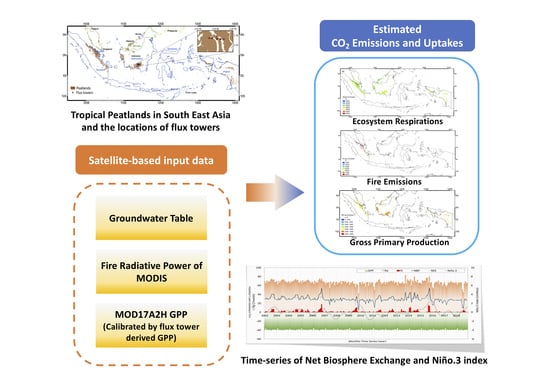
Satellite-Based Estimation of Carbon Dioxide Budget in Tropical Peatland Ecosystems


Abstract
1. Introduction
2. Materials and Methods
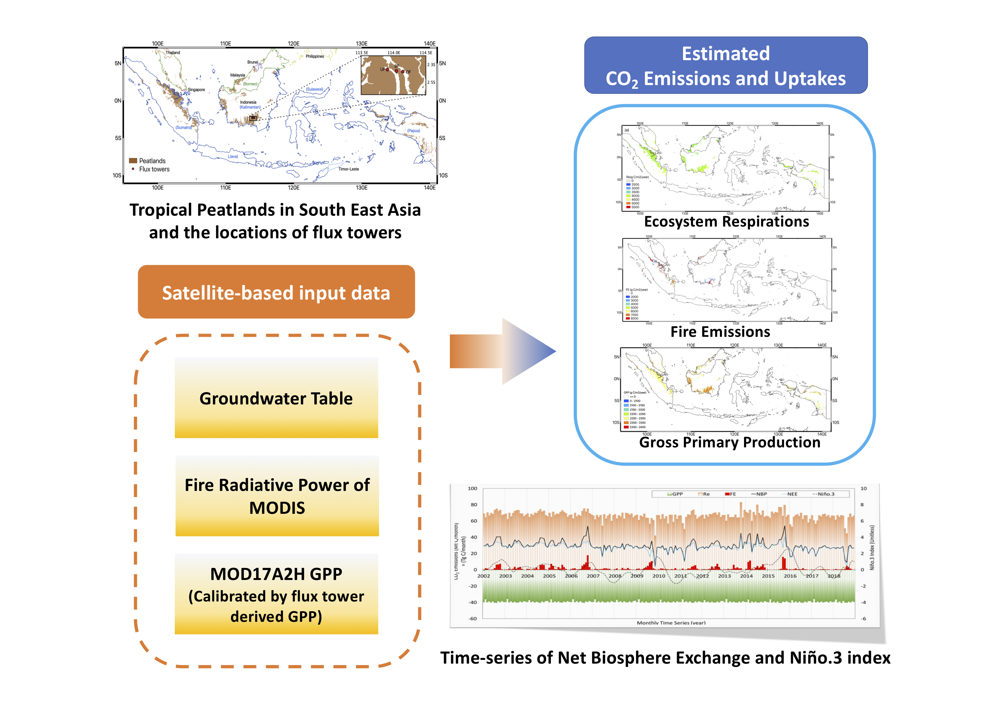
2.1. Study Area
2.2. Data
2.2.1. KBDI–Based GWT
2.2.2. Flux Tower Observations
2.2.3. MODIS GPP
2.2.4. Fire Emissions Based on MODIS
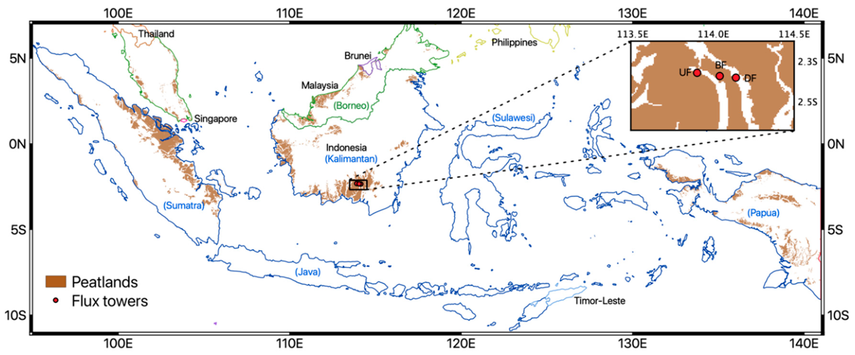
2.3. Methods
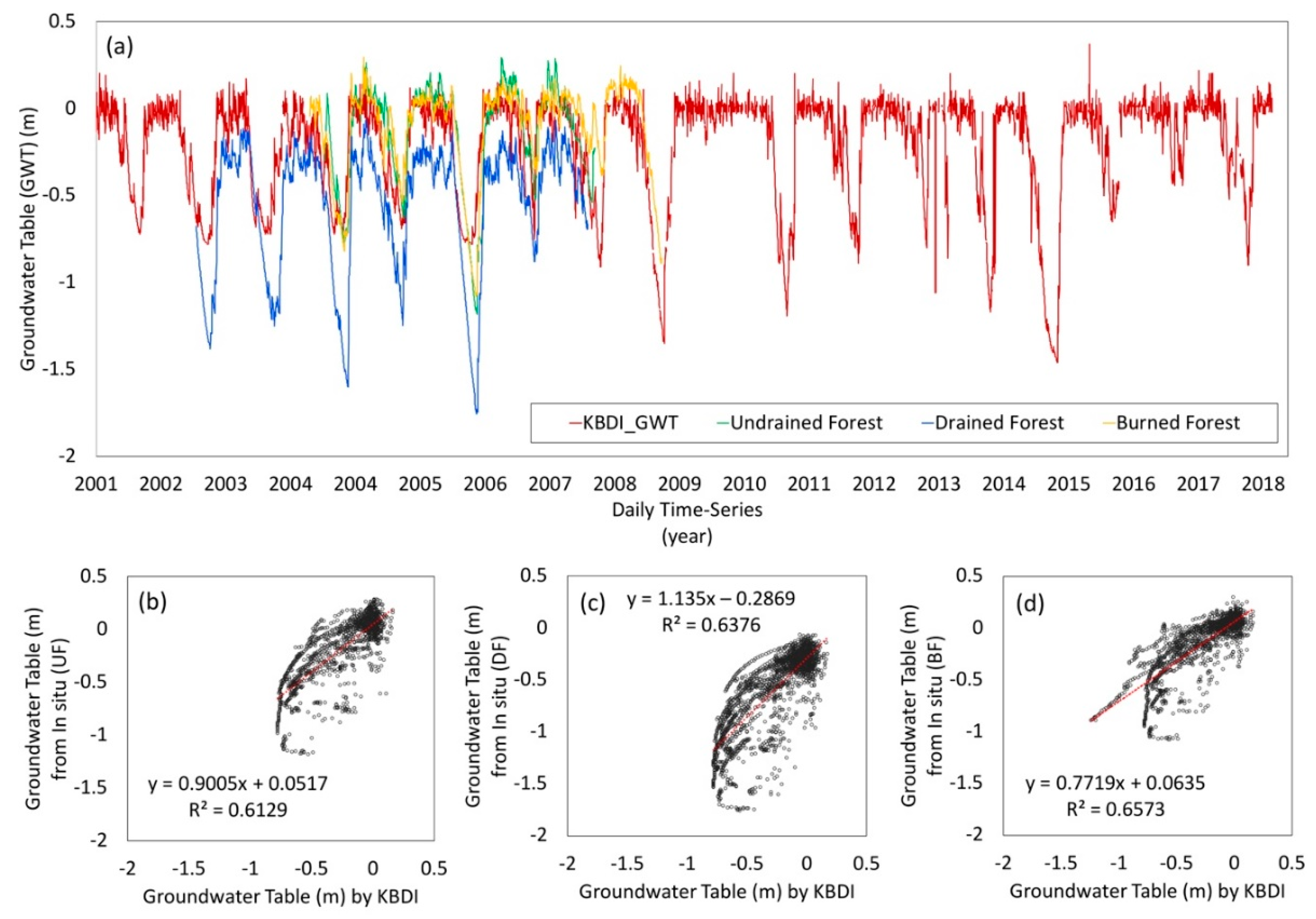
2.3.1. GWT Calculations
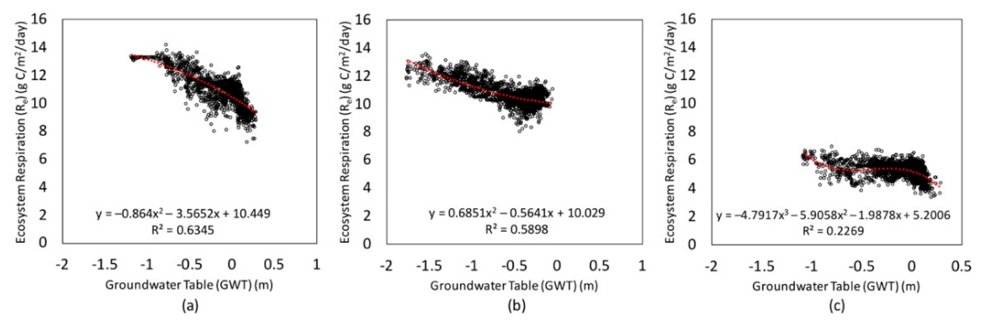
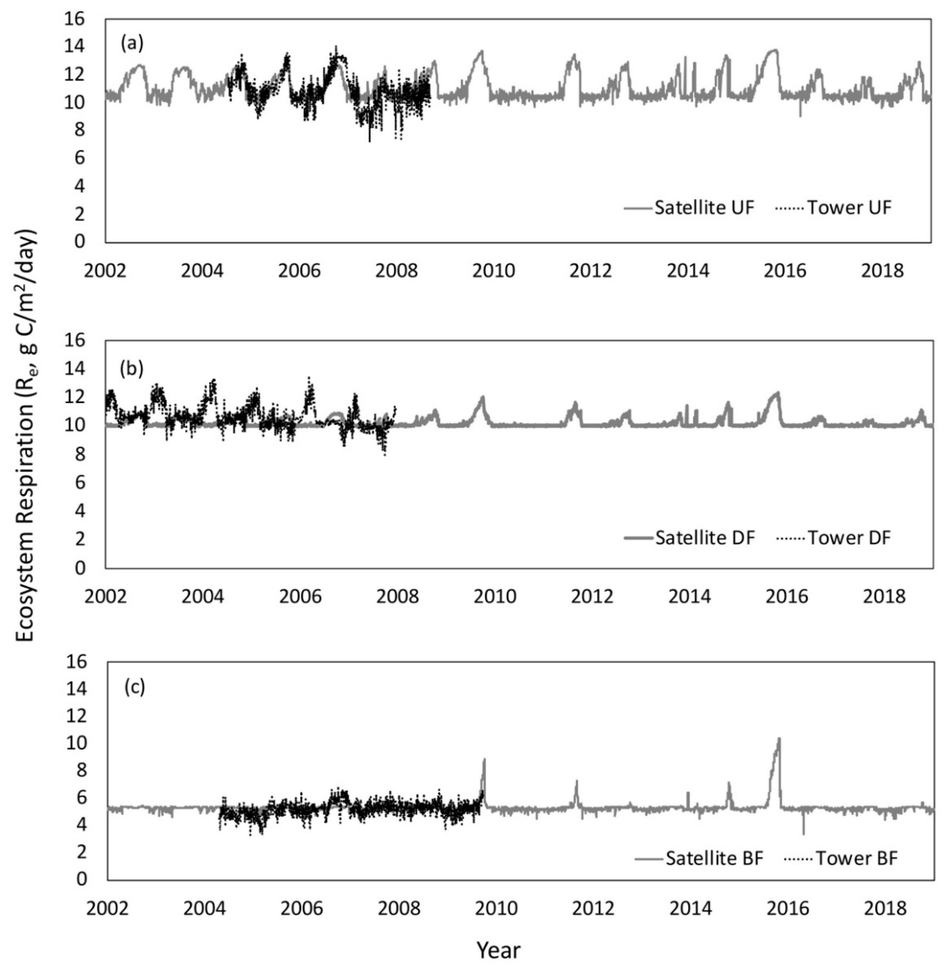
2.3.2. Ecosystem Respiration
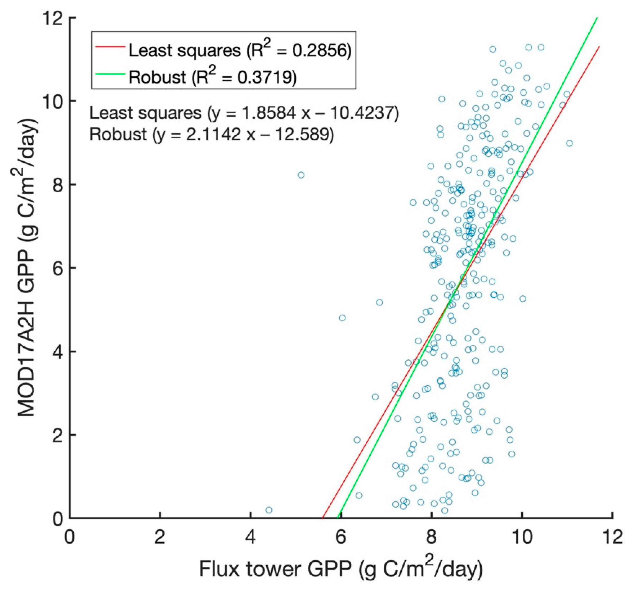
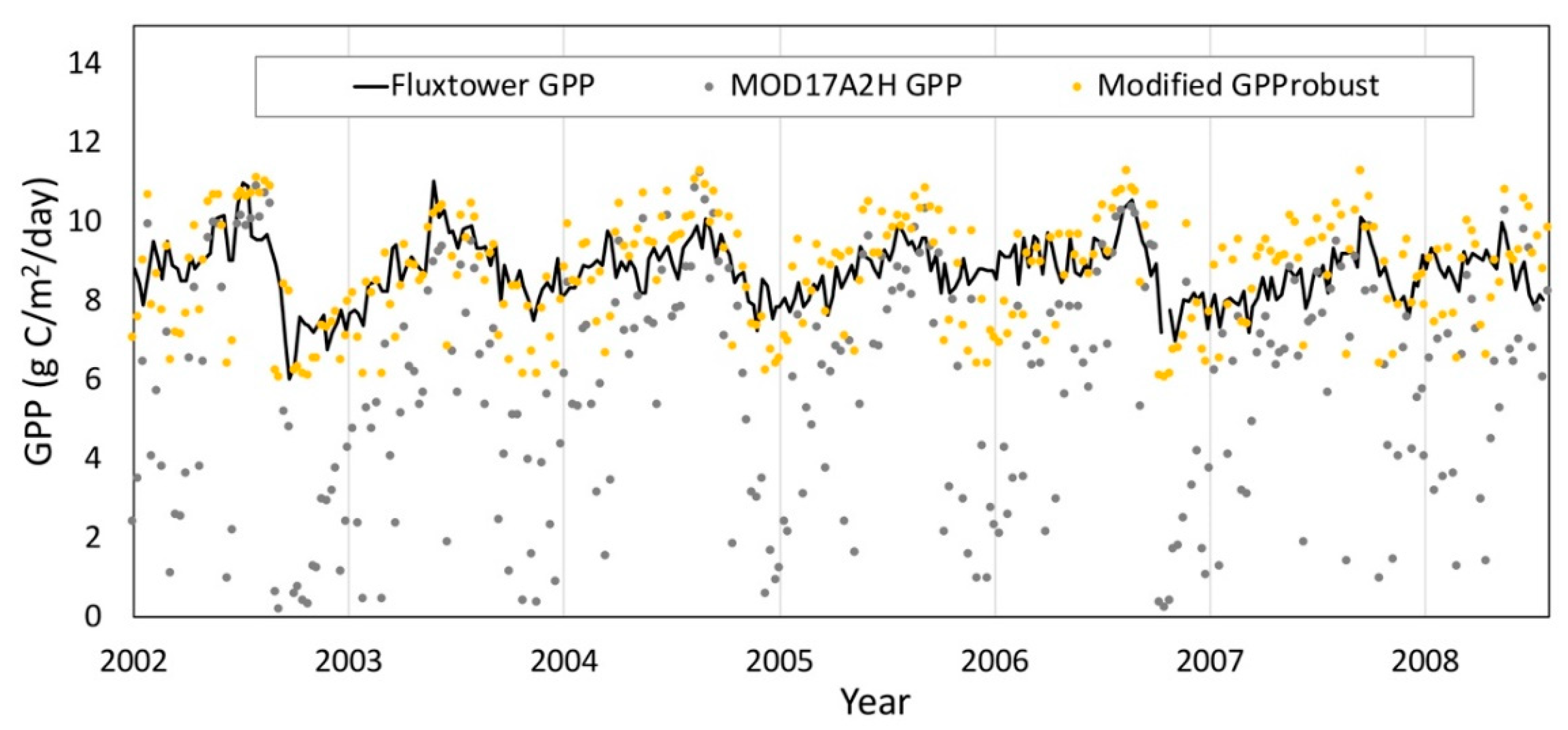
2.3.3. GPP Calibration
2.3.4. Net Biosphere Exchange
3. Results
3.1. GWT
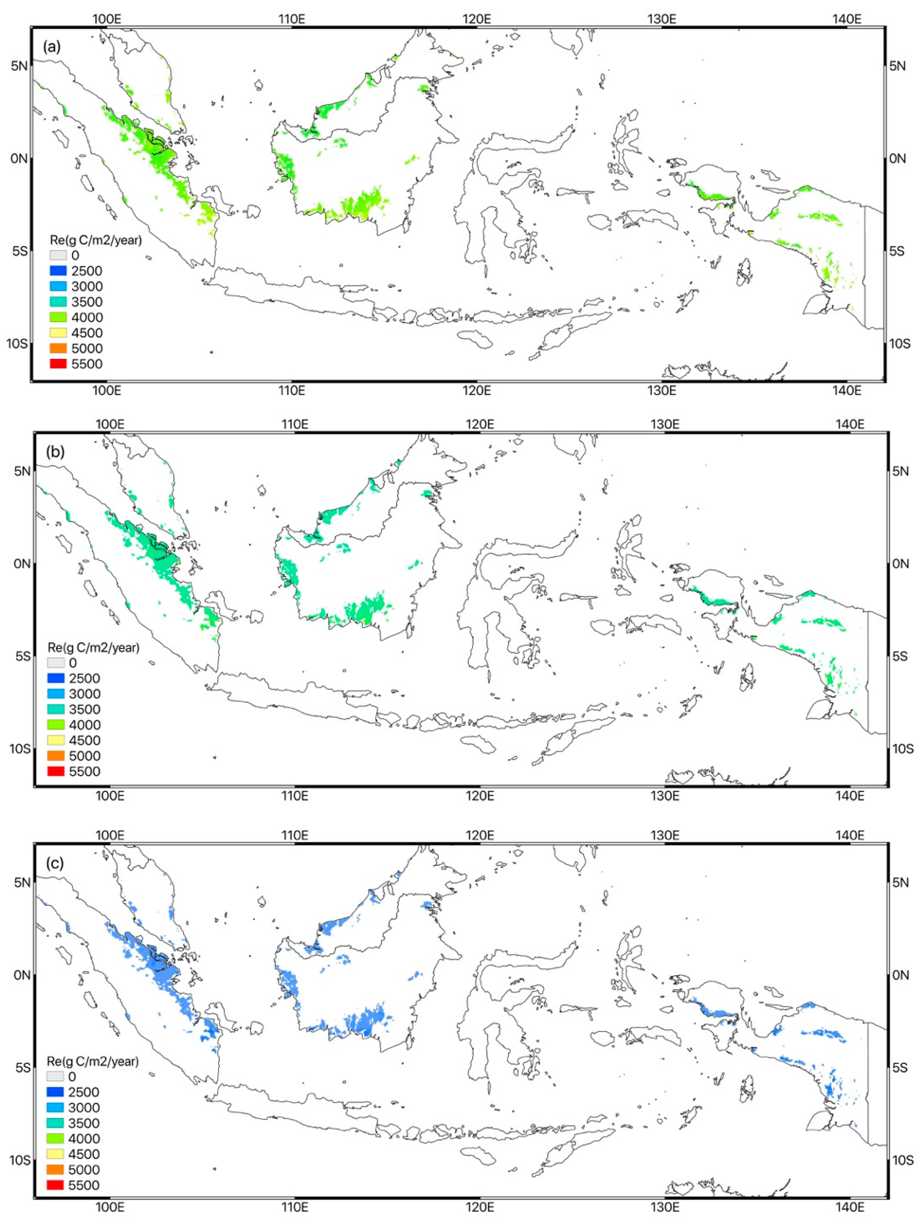
3.2. Ecosystem Respiration
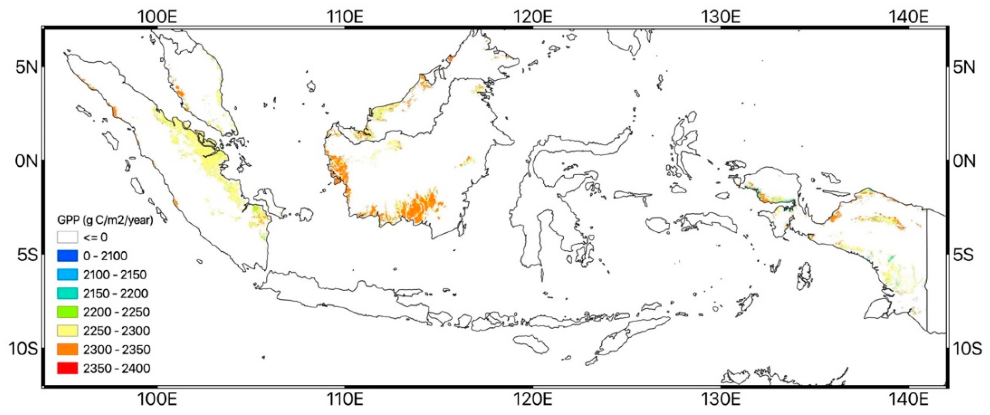
3.3. GPP in Tropical Peatlands
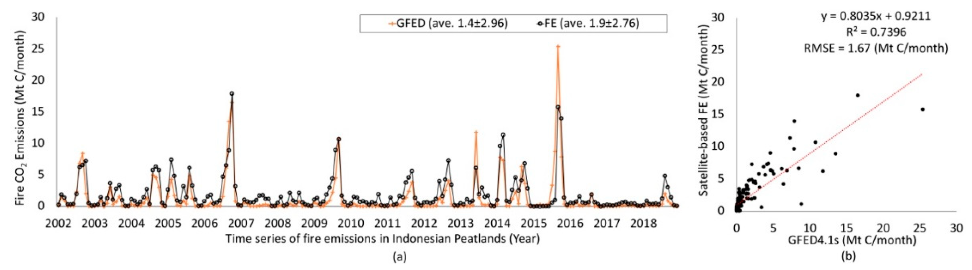
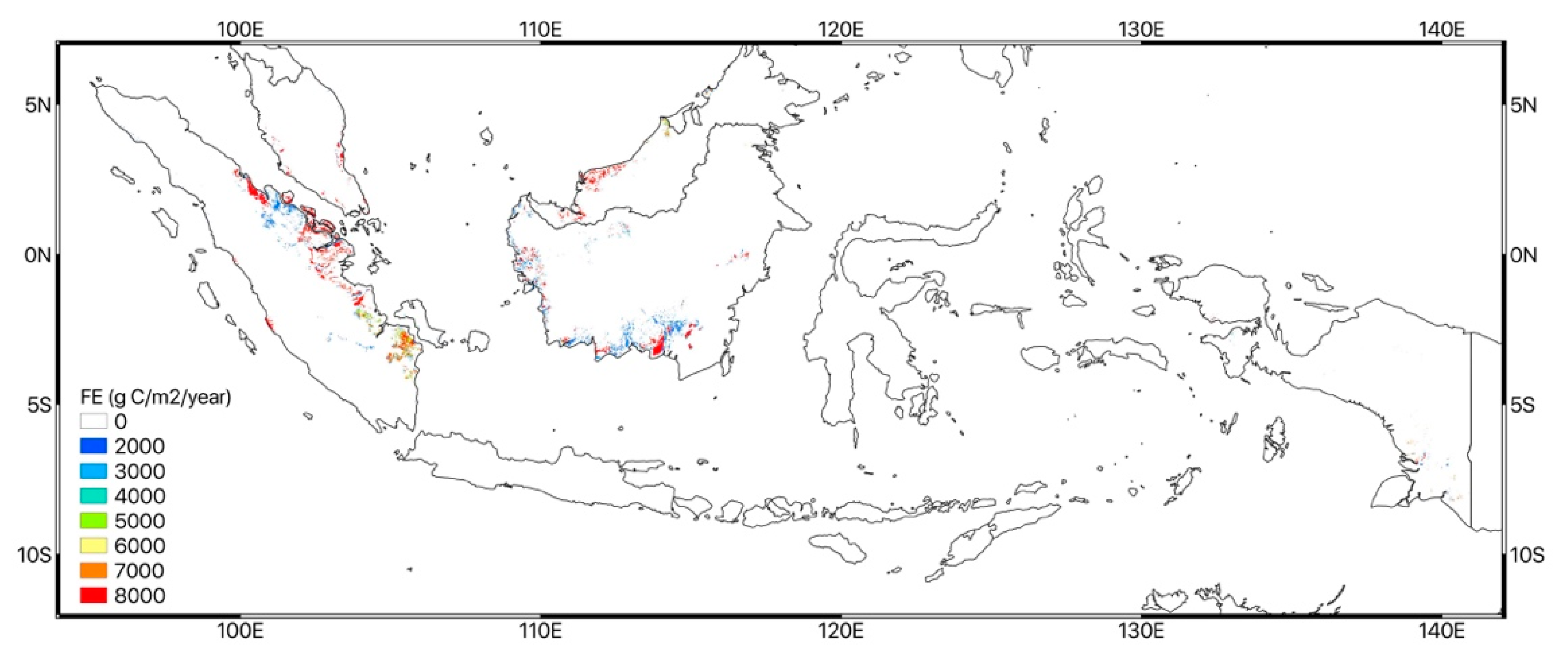
3.4. Fire Emissions
3.5. NBE Results and Validation with Flux Tower Data
4. Discussions
4.1. Spatial Distributions of GPP and Potential Uncertainties
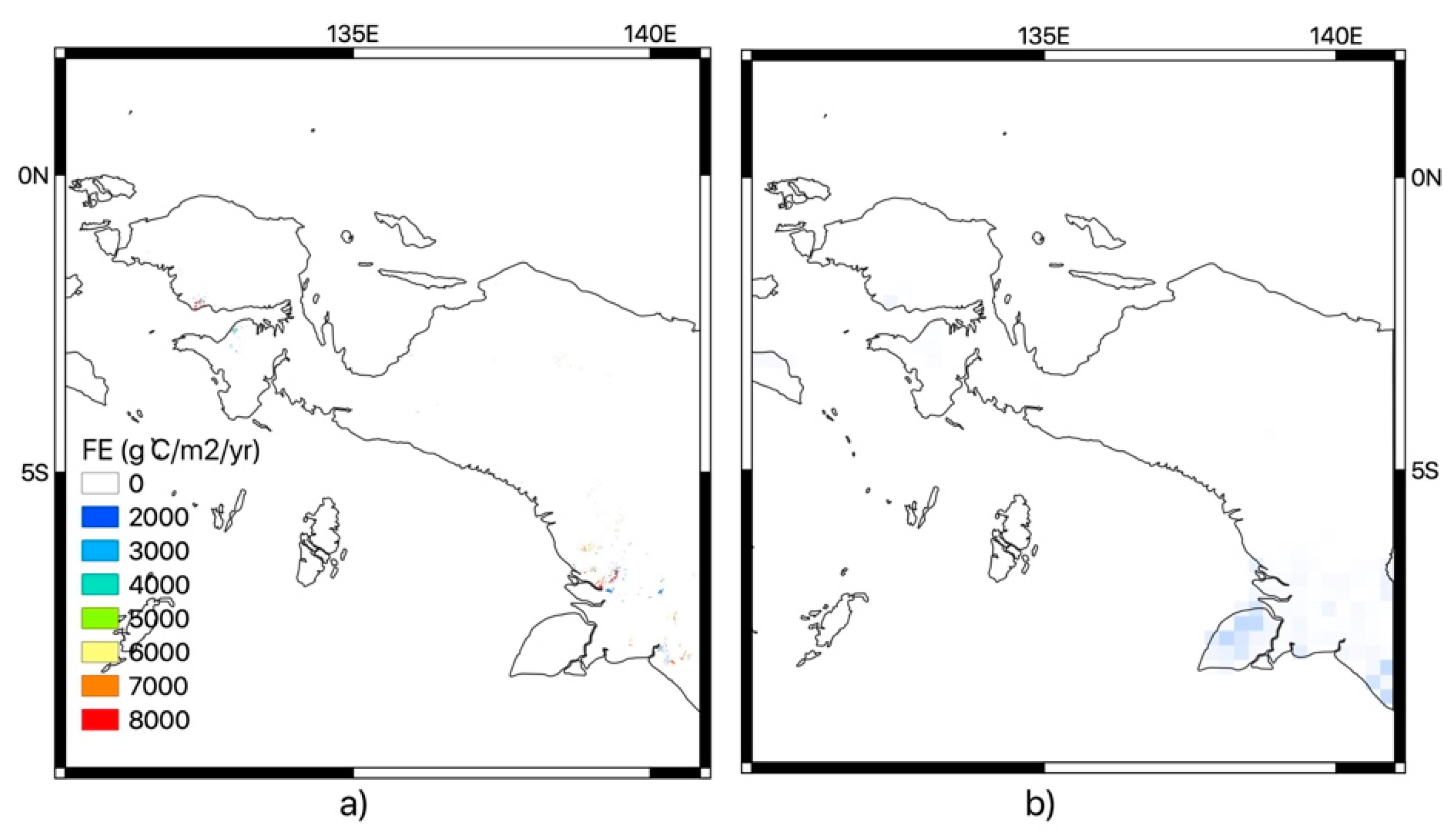
4.2. FE Comparisons with GFED 4.1s
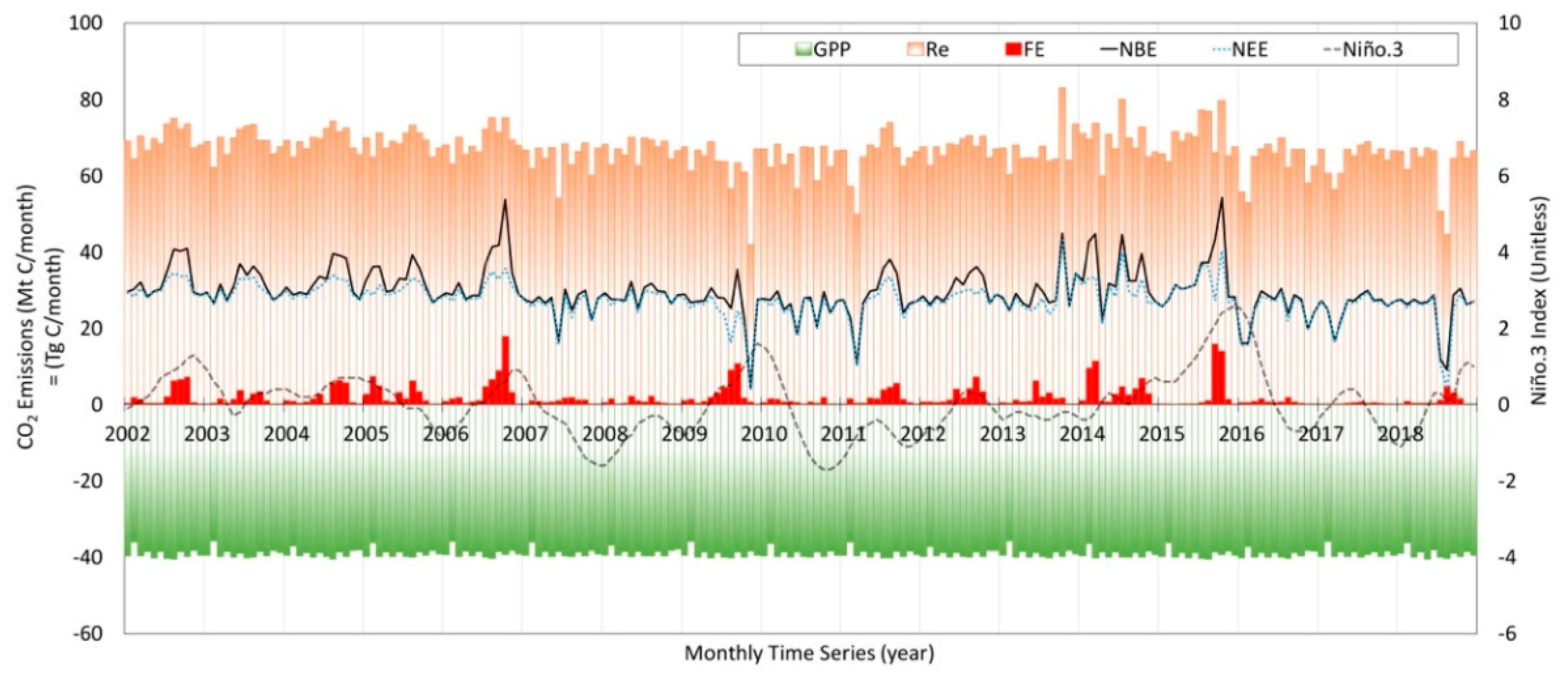
4.3. NBE and Niño.3 Index
4.4. NBE Reliability Comparing with Other Studies
5. Conclusions
Author Contributions
Funding
Acknowledgments
Conflicts of Interest
Appendix A

| Land Cover Type | Coefficient | Correlation Coefficient (R2) |
|---|---|---|
| Evergreen Needleleaf Forest | 157 | 0.50 |
| Evergreen Broadleaf Forest | 176.4 | 0.64 |
| Deciduous Needleleaf Forest | 93.1 | 0.53 |
| Deciduous Broadleaf Forest | 106.4 | 0.53 |
| Mixed Forest | 111.7 | 0.45 |
| Closed Shrublands | 110.5 | 0.49 |
| Open Shrublands | 151.3 | 0.34 |
| Woody Savannas | 133.3 | 0.42 |
| Savannas | 89.7 | 0.30 |
| Grasslands | 78.9 | 0.36 |
| Permanent Wetlands | 167.8 | 0.59 |
| Croplands | 77.9 | 0.25 |
| Urban and Built-up | 130.7 | 0.45 |
| Cropland/Natural Vegetation Mosaics | 125.4 | 0.33 |
| Permanent Snow and Ice | 271.2 | 0.39 |
| Barren | 85.6 | 0.22 |

References
- Ishikura, K.; Darung, U.; Inoue, T.; Hatano, R. Variation in soil properties regulate greenhouse gas fluxes and global warming potential in three land use types on tropical peat. Atmosphere 2018, 9, 465. [Google Scholar] [CrossRef]
- Joosten, H.; Clarke, D. Wise Use of Mires and Peatlands; International Mire Conservation Group and International Peat Society: Jyväskylä, Finland, 2002; Volume 304. [Google Scholar]
- Page, S.; Hosciło, A.; Wösten, H.; Jauhiainen, J.; Silvius, M.; Rieley, J.; Ritzema, H.; Tansey, K.; Graham, L.; Vasander, H. Restoration ecology of lowland tropical peatlands in Southeast Asia: Current knowledge and future research directions. Ecosystems 2009, 12, 888–905. [Google Scholar] [CrossRef]
- Page, S.E.; Rieley, J.O.; Banks, C.J. Global and regional importance of the tropical peatland carbon pool. Glob. Chang. Biol. 2011, 17, 798–818. [Google Scholar] [CrossRef]
- Gorham, E. Northern peatlands: Role in the carbon cycle and probable responses to climatic warming. Ecol. Appl. 1991, 1, 182–195. [Google Scholar] [CrossRef] [PubMed]
- Jaenicke, J.; Wösten, H.; Budiman, A.; Siegert, F. Planning hydrological restoration of peatlands in Indonesia to mitigate carbon dioxide emissions. Mitig. Adapt. Strateg. Glob. Chang. 2010, 15, 223–239. [Google Scholar] [CrossRef]
- Metz, B.; Davidson, O.; de Coninck, H.; Loos, M.; Meyer, L. Carbon Dioxide Capture and Storage; IPCC Special Report; Cambridge University Press: Cambridge, UK; New York, NY, USA, 2005; p. 342. [Google Scholar]
- Protocol, K. United Nations Framework Convention on Climate Change. 2011. Available online: https://unfccc.int/resource/docs/2011/sbi/eng/inf02.pdf (accessed on 9 January 2020).
- Morgan, J.; Dagnet, Y.; Tirpak, D. Elements and Ideas for the 2015 Paris Agreement; World Resources Institute: Washington, DC, USA, 2015. [Google Scholar]
- Alley, R.; Berntsen, T.; Bindoff, N.L.; Chen, Z.; Chidthaisong, A.; Friedlingstein, P.; Gregory, J.; Hegerl, G.; Heimann, M.; Hewitson, B. Climate Change 2007: The Physical Science Basis; Working Group I to the Fourth Assessment Report of the Intergovernmental Panel on Climate Change. Summary for Policymakers; IPCC Secretariat: Geneva, Switzerland, 2007. [Google Scholar]
- Page, S.; Wűst, R.; Weiss, D.; Rieley, J.; Shotyk, W.; Limin, S.H. A record of Late Pleistocene and Holocene carbon accumulation and climate change from an equatorial peat bog (Kalimantan, Indonesia): Implications for past, present and future carbon dynamics. J. Quat. Sci. 2004, 19, 625–635. [Google Scholar] [CrossRef]
- Limpens, J.; Berendse, F.; Blodau, C.; Canadell, J.; Freeman, C.; Holden, J.; Roulet, N.; Rydin, H.; Schaepman-Strub, G. Peatlands and the carbon cycle: From local processes to global implications—A synthesis. Biogeosciences 2008, 5, 1475–1491. [Google Scholar] [CrossRef]
- Hooijer, A.; Page, S.; Canadell, J.; Silvius, M.; Kwadijk, J.; Wosten, H.; Jauhiainen, J. Current and future CO2 emissions from drained peatlands in Southeast Asia. Biogeosciences 2010. [Google Scholar] [CrossRef]
- Page, S.E.; Siegert, F.; Rieley, J.O.; Boehm, H.-D.V.; Jaya, A.; Limin, S. The amount of carbon released from peat and forest fires in Indonesia during 1997. Nature 2002, 420, 61. [Google Scholar] [CrossRef]
- Sundari, S.; Hirano, T.; Yamada, H.; Kusin, K.; Limin, S. Effect of groundwater level on soil respiration in tropical peat swamp forests. J. Agric. Meteorol. 2012, 68, 121–134. [Google Scholar] [CrossRef]
- Husnain, H.; Wigena, I.P.; Dariah, A.; Marwanto, S.; Setyanto, P.; Agus, F. CO2 emissions from tropical drained peat in Sumatra, Indonesia. Mitig. Adapt. Strateg. Glob. Chang. 2014, 19, 845–862. [Google Scholar] [CrossRef]
- Couwenberg, J.; Dommain, R.; Joosten, H. Greenhouse gas fluxes from tropical peatlands in south-east Asia. Glob. Chang. Biol. 2010, 16, 1715–1732. [Google Scholar] [CrossRef]
- Miettinen, J.; Liew, S. Degradation and development of peatlands in Peninsular Malaysia and in the islands of Sumatra and Borneo since 1990. Land Degrad. Dev. 2010, 21, 285–296. [Google Scholar] [CrossRef]
- Wösten, J.; Clymans, E.; Page, S.; Rieley, J.; Limin, S. Peat–water interrelationships in a tropical peatland ecosystem in Southeast Asia. Catena 2008, 73, 212–224. [Google Scholar] [CrossRef]
- Keetch, J.J.; Byram, G.M. A Drought Index for Forest Fire Control; Res. Pap. SE-38; US Department of Agriculture, Forest Service, Southeastern Forest Experiment Station: Asheville, NC, USA, 1968; Volume 35, p. 38.
- Takeuchi, W.; Hirano, T.; Roswintiarti, O. Estimation Model of Ground Water Table at Peatland in Central Kalimantan, Indonesia. In Tropical Peatland Ecosystems; Springer: Tokyo, Japan, 2016; pp. 445–453. [Google Scholar]
- Baldocchi, D. ‘Breathing’of the terrestrial biosphere: Lessons learned from a global network of carbon dioxide flux measurement systems. Aust. J. Bot. 2008, 56, 1–26. [Google Scholar] [CrossRef]
- Yang, F.; Ichii, K.; White, M.A.; Hashimoto, H.; Michaelis, A.R.; Votava, P.; Zhu, A.-X.; Huete, A.; Running, S.W.; Nemani, R.R. Developing a continental-scale measure of gross primary production by combining MODIS and AmeriFlux data through Support Vector Machine approach. Remote Sens. Environ. 2007, 110, 109–122. [Google Scholar] [CrossRef]
- Jung, M.; Reichstein, M.; Bondeau, A. Towards global empirical upscaling of FLUXNET eddy covariance observations: Validation of a model tree ensemble approach using a biosphere model. Biogeosciences 2009, 6, 2001–2013. [Google Scholar] [CrossRef]
- Hirano, T.; Segah, H.; Kusin, K.; Limin, S.; Takahashi, H.; Osaki, M. Effects of disturbances on the carbon balance of tropical peat swamp forests. Glob. Chang. Biol. 2012, 18, 3410–3422. [Google Scholar] [CrossRef]
- Hirano, T.; Kusin, K.; Limin, S.; Osaki, M. Evapotranspiration of tropical peat swamp forests. Glob. Chang. Biol. 2015, 21, 1914–1927. [Google Scholar] [CrossRef]
- Ichii, K.; Kondo, M.; Lee, Y.-H.; Wang, S.-Q.; Kim, J.; Ueyama, M.; Lim, H.-J.; Shi, H.; Suzuki, T.; Ito, A. Site-level model–data synthesis of terrestrial carbon fluxes in the CarboEastAsia eddy-covariance observation network: Toward future modeling efforts. J. For. Res. 2013, 18, 13–20. [Google Scholar] [CrossRef]
- Ito, A. The regional carbon budget of East Asia simulated with a terrestrial ecosystem model and validated using AsiaFlux data. Agric. For. Meteorol. 2008, 148, 738–747. [Google Scholar] [CrossRef]
- Murakami, K.; Sasai, T.; Yamaguchi, Y. A new one-dimensional simple energy balance and carbon cycle coupled model for global warming simulation. Theor. Appl. Climatol. 2010, 101, 459–473. [Google Scholar] [CrossRef]
- Ueyama, M.; Ichii, K.; Hirata, R.; Takagi, K.; Asanuma, J.; Machimura, T.; Nakai, Y.; Ohta, T.; Saigusa, N.; Takahashi, Y. Simulating carbon and water cycles of larch forests in East Asia by the BIOME-BGC model with AsiaFlux data. Biogeosciences 2010, 7, 959–977. [Google Scholar] [CrossRef]
- Turner, D.; Ritts, W.; Law, B.; Cohen, W.; Yang, Z.; Hudiburg, T.; Campbell, J.; Duane, M. Scaling net ecosystem production and net biome production over a heterogeneous region in the western United States. Biogeosciences 2007, 4, 597–612. [Google Scholar] [CrossRef]
- Van der Werf, G.R.; Randerson, J.T.; Giglio, L.; Collatz, G.J.; Kasibhatla, P.S.; Arellano, A.F., Jr. Interannual variability in global biomass burning emissions from 1997 to 2004. Atmos. Chem. Phys. 2006, 6, 3423–3441. [Google Scholar] [CrossRef]
- Akagi, S.; Yokelson, R.J.; Wiedinmyer, C.; Alvarado, M.; Reid, J.; Karl, T.; Crounse, J.; Wennberg, P. Emission factors for open and domestic biomass burning for use in atmospheric models. Atmos. Chem. Phys. 2011, 11, 4039–4072. [Google Scholar] [CrossRef]
- Running, S.W.; Nemani, R.; Glassy, J.M.; Thornton, P.E. MODIS daily photosynthesis (PSN) and annual net primary production (NPP) product (MOD17) Algorithm Theoretical Basis Document. In SCF At-Launch Algorithm ATBD Documents; University of Montana: Missoula, MT, USA, 1999; Available online: https://www.ntsg.umt.edu/modis/ATBD/ATBD_MOD17_v21.pdf (accessed on 9 January 2020).
- Hansen, M.C.; Krylov, A.; Tyukavina, A.; Potapov, P.V.; Turubanova, S.; Zutta, B.; Ifo, S.; Margono, B.; Stolle, F.; Moore, R. Humid tropical forest disturbance alerts using Landsat data. Environ. Res. Lett. 2016, 11. [Google Scholar] [CrossRef]
- Global Forest Watch. Available online: www.globalforestwatch.org (accessed on 19 November 2019).
- Takeuchi, W.; Gonzalez, L. Blending MODIS and AMSR-E to predict daily land surface water coverage. In Proceedings of the International Remote Sensing Symposium (ISRS), Busan, Korea, 28–30 October 2009. [Google Scholar]
- Göckede, M.; Rebmann, C.; Foken, T. A combination of quality assessment tools for eddy covariance measurements with footprint modelling for the characterisation of complex sites. Agric. For. Meteorol. 2004, 127, 175–188. [Google Scholar] [CrossRef]
- Running, S.; Mu, Q.; Zhao, M. MOD17A2H MODIS/Terra Gross Primary Productivity 8-Day L4 Global 500m SIN Grid V006; NASA EOSDIS Land Processes DAAC: Sioux Falls, SD, USA, 2015.
- Zhao, M.; Heinsch, F.A.; Nemani, R.R.; Running, S.W. Improvements of the MODIS terrestrial gross and net primary production global data set. Remote Sens. Environ. 2005, 95, 164–176. [Google Scholar] [CrossRef]
- Andreae, M.O.; Merlet, P. Emission of trace gases and aerosols from biomass burning. Glob. Biogeochem. Cycles 2001, 15, 955–966. [Google Scholar] [CrossRef]
- Ito, A.; Oikawa, T. A simulation model of the carbon cycle in land ecosystems (Sim-CYCLE): A description based on dry-matter production theory and plot-scale validation. Ecol. Model. 2002, 151, 143–176. [Google Scholar] [CrossRef]
- Inatomi, M.; Ito, A.; Ishijima, K.; Murayama, S. Greenhouse gas budget of a cool-temperate deciduous broad-leaved forest in Japan estimated using a process-based model. Ecosystems 2010, 13, 472–483. [Google Scholar] [CrossRef]
- Takeuchi, W.; Sekiyama, A.; Imasu, R. Estimation of global carbon emissions from wild fires in forests and croplands. In Proceedings of the 2013 IEEE International Geoscience and Remote Sensing Symposium-IGARSS, Melbourne, Australia, 21–26 July 2013; pp. 1805–1808. [Google Scholar]
- Justice, C.; Giglio, L.; Korontzi, S.; Owens, J.; Morisette, J.; Roy, D.; Descloitres, J.; Alleaume, S.; Petitcolin, F.; Kaufman, Y. The MODIS fire products. Remote Sens. Environ. 2002, 83, 244–262. [Google Scholar] [CrossRef]
- Wooster, M.J.; Roberts, G.; Perry, G.; Kaufman, Y. Retrieval of biomass combustion rates and totals from fire radiative power observations: FRP derivation and calibration relationships between biomass consumption and fire radiative energy release. J. Geophys. Res. Atmos. 2005, 110. [Google Scholar] [CrossRef]
- Van der Werf, G.R.; Randerson, J.T.; Giglio, L.; Van Leeuwen, T.T.; Chen, Y.; Rogers, B.M.; Mu, M.; Van Marle, M.J.; Morton, D.C.; Collatz, G.J. Global fire emissions estimates during 1997–2016. Earth Syst. Sci. Data 2017. [Google Scholar] [CrossRef]
- Benali, A.; Carvalho, A.; Nunes, J.; Carvalhais, N.; Santos, A. Estimating air surface temperature in Portugal using MODIS LST data. Remote Sens. Environ. 2012, 124, 108–121. [Google Scholar] [CrossRef]
- Vogt, J.V.; Viau, A.A.; Paquet, F. Mapping regional air temperature fields using satellite-derived surface skin temperatures. Int. J. Climatol. 1997, 17, 1559–1579. [Google Scholar] [CrossRef]
- Rieley, J. Tropical peatland-The amazing dual ecosystem: Coexistence and mutual benefit. In Proceedings of the International Symposium and Workshop on Tropical Peatland, Leicester, UK, 27–29 August 2007; pp. 1–14. [Google Scholar]
- Verstraeten, W.W.; Veroustraete, F.; Feyen, J. On temperature and water limitation of net ecosystem productivity: Implementation in the C-Fix model. Ecol. Model. 2006, 199, 4–22. [Google Scholar] [CrossRef]
- Hansen, P.C.; Pereyra, V.; Scherer, G. Least Squares Data Fitting with Applications; JHU Press: Baltimore, MD, USA, 2013. [Google Scholar]
- Rousseeuw, P.J.; Leroy, A.M. Robust Regression and Outlier Detection; John Wiley & Sons: Hoboken, NJ, USA, 2005; Volume 589. [Google Scholar]
- He, M.; Ju, W.; Zhou, Y.; Chen, J.; He, H.; Wang, S.; Wang, H.; Guan, D.; Yan, J.; Li, Y. Development of a two-leaf light use efficiency model for improving the calculation of terrestrial gross primary productivity. Agric. For. Meteorol. 2013, 173, 28–39. [Google Scholar] [CrossRef]
- Propastin, P.; Ibrom, A.; Knohl, A.; Erasmi, S. Effects of canopy photosynthesis saturation on the estimation of gross primary productivity from MODIS data in a tropical forest. Remote Sens. Environ. 2012, 121, 252–260. [Google Scholar] [CrossRef]
- DeLUCIA, E.H.; Drake, J.E.; Thomas, R.B.; Gonzalez-Meler, M. Forest carbon use efficiency: Is respiration a constant fraction of gross primary production? Glob. Chang. Biol. 2007, 13, 1157–1167. [Google Scholar] [CrossRef]
- Hashimoto, H.; Dungan, J.L.; White, M.A.; Yang, F.; Michaelis, A.R.; Running, S.W.; Nemani, R.R. Satellite-based estimation of surface vapor pressure deficits using MODIS land surface temperature data. Remote Sens. Environ. 2008, 112, 142–155. [Google Scholar] [CrossRef]
- Li, L.; Zha, Y. Mapping relative humidity, average and extreme temperature in hot summer over China. Sci. Total Environ. 2018, 615, 875–881. [Google Scholar] [CrossRef] [PubMed]
- Robinson, N.P.; Allred, B.W.; Smith, W.K.; Jones, M.O.; Moreno, A.; Erickson, T.A.; Naugle, D.E.; Running, S.W. Terrestrial primary production for the conterminous United States derived from Landsat 30 m and MODIS 250 m. Remote Sens. Ecol. Conserv. 2018, 4, 264–280. [Google Scholar] [CrossRef]
- Ustin, S.L.; Gamon, J.A. Remote sensing of plant functional types. New Phytol. 2010, 186, 795–816. [Google Scholar] [CrossRef] [PubMed]
- Van der Werf, G.; Randerson, J.; Giglio, L.; Collatz, J.; Kasibhatla, P.; Morton, D.; DeFries, R. The improved Global Fire Emissions Database (GFED) version 3: Contribution of savanna, forest, deforestation, and peat fires to the global fire emissions budget. In Proceedings of the EGU General Assembly Conference Abstracts, Vienna, Austria, 2–7 May 2010; p. 13010. [Google Scholar]
- Brown, L.E.; Holden, J.; Palmer, S.M.; Johnston, K.; Ramchunder, S.J.; Grayson, R. Effects of fire on the hydrology, biogeochemistry, and ecology of peatland river systems. Freshw. Sci. 2015, 34, 1406–1425. [Google Scholar] [CrossRef]
- Kirono, D.G.; Tapper, N.J. ENSO rainfall variability and impacts on crop production in Indonesia. Phys. Geogr. 1999, 20, 508–519. [Google Scholar] [CrossRef]
- D’Arrigo, R.; Wilson, R. El Nino and Indian Ocean influences on Indonesian drought: Implications for forecasting rainfall and crop productivity. Int. J. Climatol. 2008, 28, 611–616. [Google Scholar] [CrossRef]
- Field, R.D.; van der Werf, G.R.; Shen, S.S. Human amplification of drought-induced biomass burning in Indonesia since 1960. Nat. Geosci. 2009, 2, 185. [Google Scholar] [CrossRef]
- Liu, J.; Bowman, K.W.; Schimel, D.S.; Parazoo, N.C.; Jiang, Z.; Lee, M.; Bloom, A.A.; Wunch, D.; Frankenberg, C.; Sun, Y. Contrasting carbon cycle responses of the tropical continents to the 2015–2016 El Niño. Science 2017, 358. [Google Scholar] [CrossRef]
- Guerlet, S.; Basu, S.; Butz, A.; Krol, M.; Hahne, P.; Houweling, S.; Hasekamp, O.; Aben, I. Reduced carbon uptake during the 2010 Northern Hemisphere summer from GOSAT. Geophys. Res. Lett. 2013, 40, 2378–2383. [Google Scholar] [CrossRef]
- He, Z.; Lei, L.; Welp, L.; Zeng, Z.-C.; Bie, N.; Yang, S.; Liu, L. Detection of Spatiotemporal Extreme Changes in Atmospheric CO2 Concentration Based on Satellite Observations. Remote Sens. 2018, 10, 839. [Google Scholar] [CrossRef]
- Holle, R.L. Effects of cloud condensation nuclei due to fires and surface sources during South Florida droughts. J. Appl. Meteorol. 1971, 10, 62–69. [Google Scholar] [CrossRef][Green Version]
- Achtemeier, G.L. On the formation and persistence of superfog in woodland smoke. Meteorol. Appl. 2009, 16, 215–225. [Google Scholar] [CrossRef]
- Davison, P.; Roberts, D.; Arnold, R.; Colvile, R. Estimating the direct radiative forcing due to haze from the 1997 forest fires in Indonesia. J. Geophys. Res. Atmos. 2004, 109. [Google Scholar] [CrossRef]
- Joosten, H. The Global Peatland CO2 Picture: Peatland Status and Drainage Related Emissions in All Countries of the World; Wetlands International: Wageningen, The Netherlands, 2010. [Google Scholar]


© 2020 by the authors. Licensee MDPI, Basel, Switzerland. This article is an open access article distributed under the terms and conditions of the Creative Commons Attribution (CC BY) license (http://creativecommons.org/licenses/by/4.0/).
Share and Cite
Park, H.; Takeuchi, W.; Ichii, K. Satellite-Based Estimation of Carbon Dioxide Budget in Tropical Peatland Ecosystems. Remote Sens. 2020, 12, 250. https://doi.org/10.3390/rs12020250
Park H, Takeuchi W, Ichii K. Satellite-Based Estimation of Carbon Dioxide Budget in Tropical Peatland Ecosystems. Remote Sensing. 2020; 12(2):250. https://doi.org/10.3390/rs12020250
Chicago/Turabian StylePark, Haemi, Wataru Takeuchi, and Kazuhito Ichii. 2020. "Satellite-Based Estimation of Carbon Dioxide Budget in Tropical Peatland Ecosystems" Remote Sensing 12, no. 2: 250. https://doi.org/10.3390/rs12020250
APA StylePark, H., Takeuchi, W., & Ichii, K. (2020). Satellite-Based Estimation of Carbon Dioxide Budget in Tropical Peatland Ecosystems. Remote Sensing, 12(2), 250. https://doi.org/10.3390/rs12020250