Towards an Operational, Split Window-Derived Surface Temperature Product for the Thermal Infrared Sensors Onboard Landsat 8 and 9

Abstract

The split window technique has been used for over thirty years to derive surface temperatures of the Earth with image data collected from spaceborne sensors containing two thermal channels. The latest NASA/USGS Landsat satellites contain the Thermal Infrared Sensor (TIRS) instruments that acquire Earth data in two longwave infrared bands, as opposed to a single band with earlier Landsats. The United States Geological Survey (USGS) will soon begin releasing a surface temperature product for Landsats 4 through 8 based on the single spectral channel methodology. However, progress is being made toward developing and validating a more accurate and less computationally intensive surface temperature product based on the split window method for Landsat 8 and 9 datasets. This work presents the progress made towards developing an operational split window algorithm for TIRS. Specifically, details of how the generalized split window algorithm was tailored for the TIRS sensors are presented, along with geometric considerations that should be addressed to avoid spatial artifacts in the final surface temperature product. Validation studies indicate that the proposed algorithm is accurate to within 2 K when compared to land-based measurements and to within 1 K when compared to water-based measurements, highlighting the improved accuracy that may be achieved over the current single-channel methodology being used to derive surface temperature in the Landsat Collection 2 surface temperature product. Surface temperature products using the split window methodologies described here can be made available upon request for testing purposes.

1. Introduction

The United States Geological Survey’s (USGS) Earth Resources Observation and Science (EROS) Center will begin distributing higher-level products derived from Landsat image data as part of their Collection 2 release in early 2020. A global surface temperature (ST) product will be included in Collection 2 and will contain over thirty-five years of data collected from the various thermal instruments onboard Landsats 4 through 8. A single-channel algorithm that utilizes the Goddard Earth Observing System, Version 5 (GEOS-5) reanalysis data for atmospheric characterization along with a radiative transfer model (e.g., MODTRAN) will be applied to the existing thermal data archive and to newly collected scenes in a near real-time fashion to produce per-pixel, 30 m surface temperature data [1,2]. On the other hand, the recent Landsat 8 and upcoming Landsat 9 missions both contain the dual-band Thermal Infrared Sensor (TIRS) [3] that will enable the use of the split-window surface temperature algorithm. Recent software updates to the Landsat 8/TIRS image processing flow have mitigated the adverse effects of the stray light issue [4] that precluded the use of the split-window method. Once the radiometric quality of TIRS image data had been brought back to within requirements, work began on developing a split window algorithm tailored to TIRS image data. Several considerations were addressed before using data from these instruments to derive Earth surface temperature with the more accurate and computationally attractive split window algorithm.

This paper presents progress made towards developing and verifying an operational version of the split window algorithm for the TIRS instruments. Specifically, a discussion of the radiometric performance of the split window algorithm versus the single channel methodology implemented in the Collection 2 release is provided with ground-based measurements used as a baseline for reference. Surface measurements from several sites across the continental United States and near-shore and inland buoys were used to demonstrate the improved radiometric performance that may be achieved in future releases of ST products using dual-band Landsat thermal instruments.

An additional discussion regarding the spatial fidelity of split window-derived versus single channel-derived surface temperature products is also provided. Due to the physical layout of the TIRS focal plane, the two thermal channels, Band 10 and Band 11, acquire scene content at slightly different times. As such, an inherent misregistration of image data is evident in the corresponding Level 1 radiance product. Although band-to-band registration is well-within the defined specification [5], applying the difference terms in the split window algorithm (see Equation (1)) leads to undesired artifacts in the resulting surface temperature product. The origin of, and strategies to mitigate, these artifacts are presented along with future considerations necessary to achieve an operational split window product from Landsat 8 and 9 TIRS image data for Collection 3 processing.

2. Methodologies

Leveraging over twenty years of knowledge and refinements, the split window algorithm used in this work was initially proposed by Becker and Li, (1990) for the AVHRR instrument [6]. Wan and Dozier, (1996) generalized the algorithm to enable its utility for other dual-band instruments with a final adjustment made by Wan, (2014) to improve its performance over bare soils for the MODIS instruments [7,8]. The final form of the split window algorithm used here is

$$ST=b_0+\left(b_1+b_2\frac{1-ϵ}{ϵ}+b_3\frac{\Delta ϵ}{{ϵ}^2}\right)\frac{T_i+T_j}{2}+\left(b_4+b_5\frac{1-ϵ}{ϵ}+b_6\frac{\Delta ϵ}{{ϵ}^2}\right)\frac{T_i-T_j}{2}+b_7{(T_i-T_j)}^2,$$

(1)

where

• ST is the desired surface temperature [K];
• b_k (for k = 0, 1, …, 7) are sensor-dependent (and potentially water-vapor-dependent) coefficients that are derived through a training process;
• i and j correspond to the two thermal bands (Bands 10 and 11 for TIRS);
• $\Delta ϵ={ϵ}_i-{ϵ}_j$ or the difference in band-effective emissivities;
• $ϵ=({ϵ}_i+{ϵ}_j$)/2 or the average of the band-effective emissivities;
• T_i, T_j are the apparent temperatures in the two thermal bands.

Once the b-coefficients are derived for a sensor of interest, the ST can be estimated from dual-band thermal image data using Equation (1) if the effective emissivity in each band is known (or can be estimated). This section provides the details of a prototype split window implementation developed for the Landsat 8/TIRS and Landsat 9/TIRS-2 sensors and a corresponding validation effort conducted thus far for Landsat 8/TIRS.

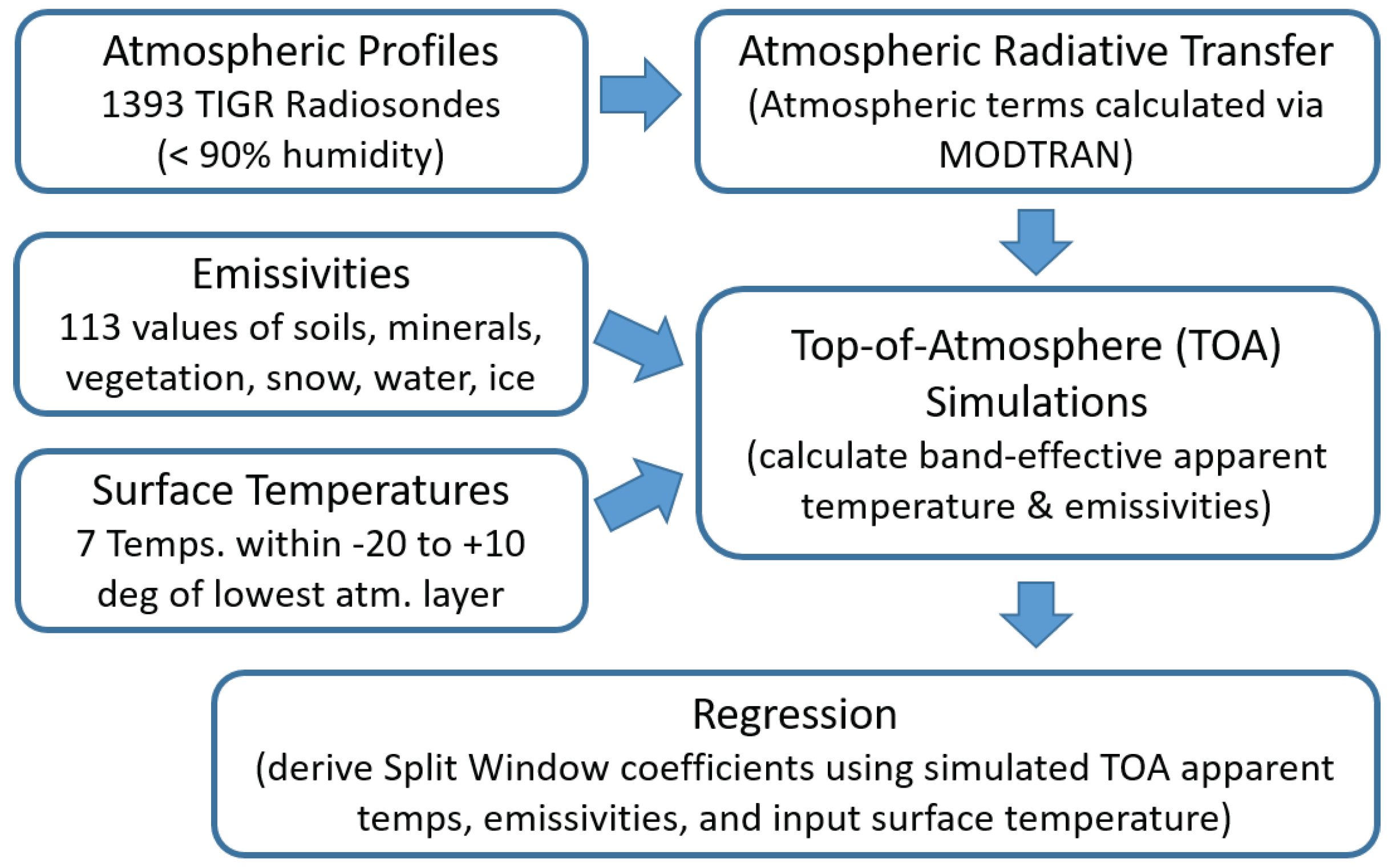
2.1. Derivation of the b-Coefficients

The flowchart in Figure 1 illustrates the training process that was performed to derive the b-coefficients shown in Equation (1). The radiative transfer model, MODTRAN [9], was used to simulate a representative range of environmental acquisition parameters. Atmospheric profiles from the Thermodynamic Initial Guess Retrieval (TIGR) database [10] were used to characterize atmospheric effects; seven surface temperatures bracketing the temperature of the lowest layer of each atmospheric profile were used as input [6,7]; and spectral emissivities of natural materials were obtained from the MODIS UCSB emissivity library [11].

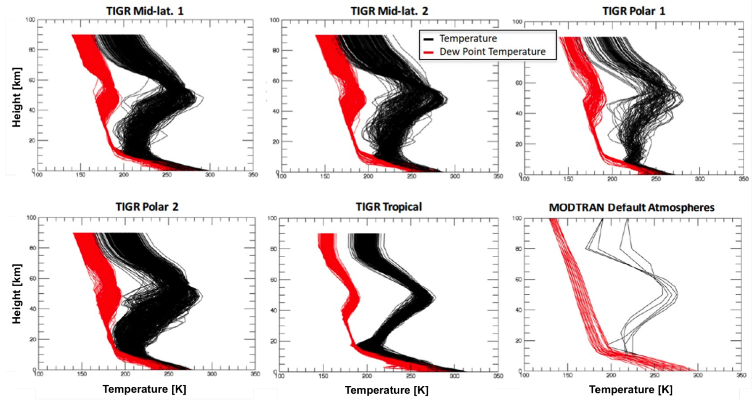
The TIGR database is a climatological library of 2311 unique atmospheric profiles that were categorized from 80,000 radiosondes. The profiles are classified into air masses (i.e., Tropical, Mid-lat1, Mid-lat2, Polar1, Polar2) that are consistent with MODTRAN’s default atmospheres but provide a richer and more densified representation of potential atmospheric effects that may be observed from a spaceborne platform. Temperature, water vapor, and ozone data are delivered at 43 predefined pressure levels ranging from 1013 mb (millibars) to 0.0026 mb [10]. Figure 2 shows plots of the 2311 atmospheric profiles provided in the TIGR database categorized by airmass. For comparison, Figure 2 (bottom right) shows the default MODTRAN profiles.

To be consistent with previous efforts and to satisfy the assumption that split window is most appropriate to be used for surface temperature retrieval when the ground temperature is close to the air temperature [6,7], seven surface temperatures bracketing the temperature of the lowest layer of each atmospheric profile were used as input to the forward model. Surface temperatures between −10 °C < t₀ < 20 °C in 5 °C steps were used in this study, where t₀ is the temperature of the lowest atmospheric layer. While some specific applications may warrant an extension of the range used to train the model (e.g., studies of urban heat island), the traditional range used here is appropriate for natural materials.

The MODIS UCSB emissivity database was used to provide a representative range of natural materials as input to the forward model [11]. With 74 unique soils and minerals, 28 unique types of vegetation, and 11 forms of water (including snow and ice), this database provides 113 unique spectral emissivities between 8 and 14 μm that can be used to train the model in Equation (1). Note that man-made materials are included in the MODIS UCSB emissivity database but were excluded in this study as the TIRS instrument has a spatial resolution of 100 m and was designed for environmental applications.

Referring again to Figure 1, all parameters described above were provided as input to a forward model that uses MODTRAN for the atmospheric radiative transfer process to generate at-sensor spectral radiance. At-sensor, band-effective radiance was calculated by sampling the simulated top-of-atmosphere spectra with the TIRS spectral response functions, and apparent temperatures (T_i, T_j) were determined by developing and utilizing a predefined look-up table that relates band-effective radiance to blackbody temperature for Bands 10 and 11 of TIRS. Finally, band-effective emissivities were calculated by sampling the 113 spectral emissivities with the TIRS spectral response functions.

Note from Figure 1 that modeled data were filtered to only include scenarios where the relative humidity is less than 90%. This was performed to remain consistent with previous studies [12] and to eliminate saturated atmospheric conditions, which represents a challenging scenario for ST retrieval. Future work will explore and include higher humidity cases as needed. Nevertheless, with all the components of Equation (1) determined, ST was regressed against the independent variables to determine the b-coefficients that best fit the model in a least-squares sense.

Table 1. Split window algorithm b-coefficients derived in this study compared the coefficients derived by Du et al. and the associated root mean square error of the model fits.

	b0	b1	b2	b3	b4	b5	b6	b7	RMSE [K]
Du et al. (2015)	−0.4117	0.0052	0.1454	−0.2730	4.0666	−6.9251	−18.2764	0.2447	0.87
Proposed Prototype	2.2925	0.9929	0.1545	−0.3122	3.7186	0.3502	−3.5889	0.1825	0.73

shows a comparison of the b-coefficients derived in this study versus the b-coefficients derived in Du et al. (2015) [12], along with the residual retrieval error when these coefficients are applied to the simulated data. Note that although the same split window algorithm was used, the derived b-coefficients could be significantly different due to the desired application. For example, Du et al. incorporated man-made materials into their training process to enable the utility of split window applications over urban areas. The impact of this training methodology on environmental applications is discussed in Section 3 and Section 4.

2.2. Emissivity Estimation

Once the b-coefficients are derived, estimation of emissivity remains the one unknown in Equation (1). To be consistent with the single channel methodology used to derive Landsat surface temperature products in the Collection 2 release, the algorithm used to estimate broadband emissivity in the existing single channel workflow was mirrored in this study but extended for the TIRS dual-band instrument. To summarize the existing workflow, ASTER emissivity products that spatially cover the Landsat scene of interest are ingested and a spectral adjustment is made to estimate the equivalent TIRS emissivities. The spectrally-adjusted emissivities are then modified based on observed in-scene conditions (e.g., emissivities may be modified if snow or vegetation is present in a scene).

The ASTER global emissivity dataset (ASTER-GED) v3 contains worldwide emissivity maps at 100 m spatial resolution. The dataset was compiled using clear-sky scenes acquired between 2000 and 2008. Emissivities were calculated with the temperature emissivity separation algorithm (TES) and the water vapor scaling (WVS) atmospheric correction algorithm, and are available for all five ASTER TIR bands centered at 8.3, 8.6, 9.1, 10.6, and 11.3 μm. The ASTER-GED has been validated to an absolute band error of 1% [13].

To enable an adjustment of the ASTER emissivities to the spectral response of the TIRS bands, a linear relationship that relates ASTER-observed (Bands 13 and 14) to TIRS-estimated (Bands 10 and 11) emissivities was developed. Note that ASTER Bands 13 and 14 were used here as they have the most overlap (spectrally) with the TIRS bands. To develop this relationship, the 113 spectral emissivities from the MODIS UCSB emissivity database described in Section 2.1 were used. Band-effective emissivities for Bands 10 and 11 of TIRS were regressed against the corresponding band-effective emissivities for Bands 13 and 14 of ASTER to derive the coefficients shown in Equations (2) and (3).

$$\begin{array}{cc}\hfill {ϵ}_{10}& =c_0+c_1{ϵ}_{13}+c_2{ϵ}_{14}\hfill \end{array}$$

(2)

$$\begin{array}{cc}\hfill {ϵ}_{11}& =c_0+c_1{ϵ}_{13}+c_2{ϵ}_{14}\hfill \end{array}$$

(3)

where,

$$\begin{array}{cc}\hfill (c_0,c_1,c_2)& =(0.6820,0.2578,0.0584)\mathrm{for}\mathrm{TIRS}\mathrm{Band}10,\hfill \\ \hfill (c_0,c_1,c_2)& =(-0.5415,1.4305,0.1092)\mathrm{for}\mathrm{TIRS}\mathrm{Band}11.\hfill \end{array}$$

Note that an estimation of the residual errors associated with these relationships can be made by applying Equations (2) and (3) to the band-effective ASTER data for the 113 emissivities. The residual errors between the estimated band-effective emissivities can then be compared to the actual band-effective emissivities (as modeled here). The standard deviations of the residual emissivities in this simulated context are 0.001 (0.1%) and 0.005 (0.5%) for Bands 10 and 11, respectively.

Since the ASTER emissivity database represents averages over a nine-year period, modifications were made to the spectrally adjusted emissivities based on observations made by the Operational Land Imager (OLI), the TIRS reflective band counterpart onboard Landsat 8. Specifically, per-pixel normalized difference vegetation indices (NDVI) and normalized difference snow indices (NDSI) were calculated with the OLI. NDSI was computed by dividing the difference in reflectance observed in the Landsat 8 green band (0.53–0.59 μm) and the shortwave infrared band (1.57–1.65 μm) by the sum of the two bands [14]. To make the NDVI adjustment, bare soil locations were estimated when the ASTER NDVI data were less than 0.1, and the Landsat vegetation emissivities adjusted accordingly based on the Landsat calculated NDVI. Snow locations for NDSI were set to 0.9876 and 0.9724 respectively for Band 10 and Band 11, where the calculated NDSI was larger than 0.4. A comprehensive description of the adjustments can be found in Malakar et al. (2018) [1].

2.3. Surface Reference Data Sources

Several sources of surface measurements were used as reference to validate the efficacy of the split window algorithm as trained here for Landsat’s TIRS instruments. Several land-based instrumented sites, including three sites from the SURFRAD [15] network and one site from the Ameriflux [16] network, were used in the assessment. Additionally, the National Oceanic and Atmospheric Administration (NOAA) buoy network [17] and the NASA Jet Propulsion Laboratory (JPL) instrumented buoys [18,19] were used to provide reference data over water.

NOAA established the surface radiation budget observing network (SURFRAD) to provide accurate, high-quality broadband solar and thermal upwelled and downwelled irradiance to support climate research, satellite retrieval validation and modeling, and weather forecasting research [15]. The current SURFRAD network consists of seven locations selected to represent diverse climates in the United States [15]. Note that three sites were chosen for this initial analysis due to their high spatial uniformity across an extended region. The three sites consist of agricultural land (Goodwin, Mississippi, US), bare soil (Desert Rock, Nevada, US), and grassland with a high inter-annual variation of snow cover (Fort Peck, Montana, US).

Each SURFRAD site is equipped with two Eppley Precision Infrared Pyrgeometers (model PIR) to collect measurements of broadband (4–50 μm) thermal infrared irradiance. The PIR pyrgeometers have a field-of-view (FOV) of 180 degrees and measure longwave irradiance with an uncertainty of ∼1.5% [20], which leads to a reported uncertainty of less than 1 K in the retrieved LST [21]. One pyrgeometer is upward facing and the other is downward facing to measure downwelled atmospheric irradiance and upwelled surface-leaving irradiance, respectively. Data from 1998 to 2009 were collected every three minutes, and every minute thereafter. The data has a quality flag to indicate failed internal quality checks. A detailed description of the SURFRAD instrumentation at each site can be found at: https://www.esrl.noaa.gov/gmd/grad/surfrad/overview.html.

FLUXNET is a vast global network of more than 800 sites for in-situ flux measurement. Regional networks contribute to the FLUXNET data, one of which is a group of sites across the Americas called AmeriFlux. There are hundreds of AmeriFlux sites, with 44 flagged as “core” sites. These core sights deliver timely data, receiving support from the AmeriFlux Management Project (AMP) to ensure high quality data collection at 30 min intervals. Since not all sites measure upwelled and downwelled thermal radiation, the core sights were filtered for spatial uniformity, activity between 2013 to 2018, and having a sufficient number of upwelled and downwelled infrared observations. Only one site passed these criteria; namely, the University of Michigan Biological Station (UMBS) [22]. This site is located within a protected forest of mid-aged northern hardwoods, conifer understory, aspen and old growth hemlock. The UMBS AmeriFlux site is equipped with a CG4 pyrgeometer from Kipp and Zonen to measure broadband (4.5 to 42 μm) thermal irradiance. The CG4 pyrgeometer, similar to the SURFRAD instrumentation, has an FOV of 180 degrees with an instrument uncertainty of less than 3% [20], and temperature uncertainty of ±0.02 K [23].

To estimate the in-situ ST using SURFRAD and AmeriFlux networks, the Stefan–Boltzmann law is manipulated to derive the following relationship [15]:

$$S{T}_{ground}={\left[\frac{1}{ϵ\sigma }(E_{upwelled}-(1-ϵ)E_{downwelled})\right]}^{\frac{1}{4}}\left[\mathrm{K}\right]$$

(4)

where ϵ represents the broadband emissivity, $\sigma =5.67·{10}^{-8}\left[\frac{\mathrm{W}}{{\mathrm{m}}^2{\mathrm{K}}^4}\right]$ is the Stefan–Boltzmann constant, and E is the measured irradiance $\left[\frac{\mathrm{W}}{{\mathrm{m}}^2}\right]$. Broadband emissivity can be retrieved from narrowband satellite emissivities via empirical relationships (Wang et al., 2005) [24]. However, this approach uses a combination of broadband emissivity from 8 to 12 μm and 14 to 25 μm. The latter range is from an emissivity library containing only measurements of minerals and does not include data beyond 25 μm because of the strong atmospheric absorption and weak thermal signals. For these reasons, the average emissivity of TIRS Bands 10 and 11 that is estimated from image data (as described in Section 2.2) was used in Equation (4) for this analysis.

When used in conjunction with land-based measurements, water represents a desirable target for surface temperature validation, as its emissivity is spectrally stable and well-defined [25]. NOAA operates a suite of worldwide instrumented buoys that collect, among other variables, water temperature. The data are freely available and delivered through their National Data Buoy Center website [17]. Measurements from thirty-six buoys in the near-shore of the United States coastline were used as reference in this work, with a bulk to surface adjustment, since measurements are obtained at depth [26]. Note that Zeng et al. (1999) estimate the uncertainty in skin temperature estimation to be approximately 0.35 K, which includes measurement uncertainty.

In addition to the NOAA sensor suite, NASA’s Jet Propulsion Laboratory’s (JPL) instrumented buoys located in Lake Tahoe, California and Salton Sea, California are attractive sources of reference data. Lake Tahoe is approximately 1900 m above sea level, and with average lake temperatures ranging from 5 to 25 °C throughout the year [18], it is an attractive cold water target for surface temperature validation. Alternatively, Salton Sea is located in Southern California and is approximately 70 m below sea level. With lake temperatures exceeding 35 °C, it is an attractive warm water target [19]. The JPL data used for the validation efforts presented here are made freely available by JPL [18,19].

Referring to

Table 2. A list of the reference data sources along with the number of measurements utilized for this work.

Site Name	Number of Sites	Number of Measurements
SurfRad	3 land sites	727
AmeriFlux	1 land site	186
NOAA Buoys	36 bouys	308
Lake Tahoe (JPL)	4 buoys	234
Salton Sea (JPL)	1 buoy	63
Total		1518

, over 1500 Landsat Level-1 Terrain-Corrected (L1T) TIRS scenes acquired between 2013 and 2018 were processed with the split window algorithm and the derived surface temperatures compared to reference measurements acquired from the various sites during the Landsat 8 overpass. For comparison, and to gauge the fidelity of the presented split window implementation, the same L1T scenes were processed to surface temperature using split window with the b-coefficients suggested by Du et al. (2015) [12] and using the single channel methodology [1] that will be delivered to users in Collection 2.

2.4. Geometric Considerations

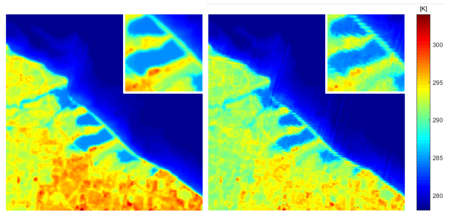
An initial application of Equation (1) to the TIRS (L1T) image data resulted in undesirable artifacts in the final surface temperature product; see an example of Lake Ontario, NY in Figure 3. The ST product derived from the single channel method is shown on the left for visual reference, while the split window-derived surface temperature image is shown on the right. Clearly, ringing artifacts can be observed at sharp transitions (edges) in the data; e.g., along the Lake Ontario shoreline as shown in the zoom windows of Figure 3. Note that the derived surface temperatures in the single channel method are roughly two degrees warmer than the temperature derived from the split window method. This discrepancy will be discussed further in Section 3.

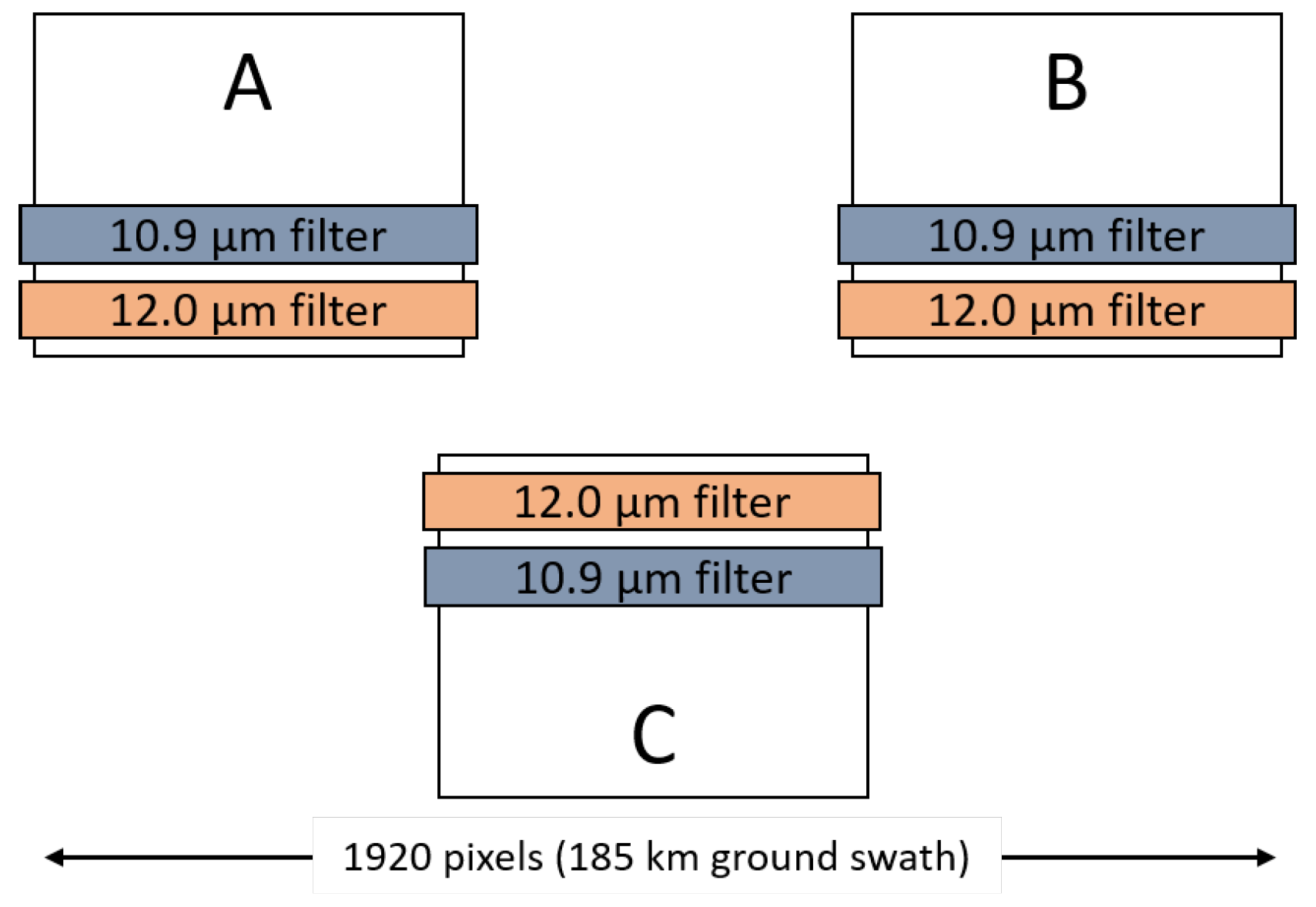
To understand the source of these artifacts, a brief background of the TIRS focal plane is required. Referring to Figure 4, the TIRS focal plane array (FPA) consists of three staggered detector arrays to cover the 185 km cross-track FOV of the instrument at a ground sampling distance (GSD) of approximately 100 m. Spectral filters are placed on the FPA detectors to produce detector rows with the desired spectral band shapes (Band 10 centered at 10.9 μm and Band 11 centered at 12.0 μm). When imaging in the nominal pushbroom mode, image data are recorded from one row of detectors in each filtered region and an image interval of the Earth is assembled as the instrument travels in orbit. Although band-to-band registration is well-within the defined specification for TIRS [5], the physical layout of the detector arrays along with the read-out sample timing in the along-track direction leads to an inherent misregistration between the Band 10 and Band 11 images. This amounts to an along-track offset of the instantaneous fields-of-view (IFOV) of the detectors in the two bands (note that the magnitude of the offset is much less than the size of the pixel). The TIRS 100-m image data is upsampled to 30 m data in the final step of the Landsat product generation process in order to match the spatial resolution of the OLI sensor. The process of upsampling exacerbates the misregistration offsets due to the fact that the along-track band offset is now a significant fraction of the 30 m pixel. When the differences between the band images are calculated as part of the split window algorithm, the along-track offsets become magnified in the product.

From a technical perspective, applying and delivering a split window-derived ST product at the nominal TIRS resolution (100 m) represents an ideal scenario to avoid artifacts introduced by the algorithm and the upsampling. However, achieving this solution would require a significant deviation from the existing EROS processing pipeline and would result in a product that differs in resolution from the other products (e.g., surface reflectance) being released in Collection 2. Alternative solutions that mitigate the spatial artifacts, yet preserve radiometric fidelity and the 30-meter resolution of the ST product, have been investigated.

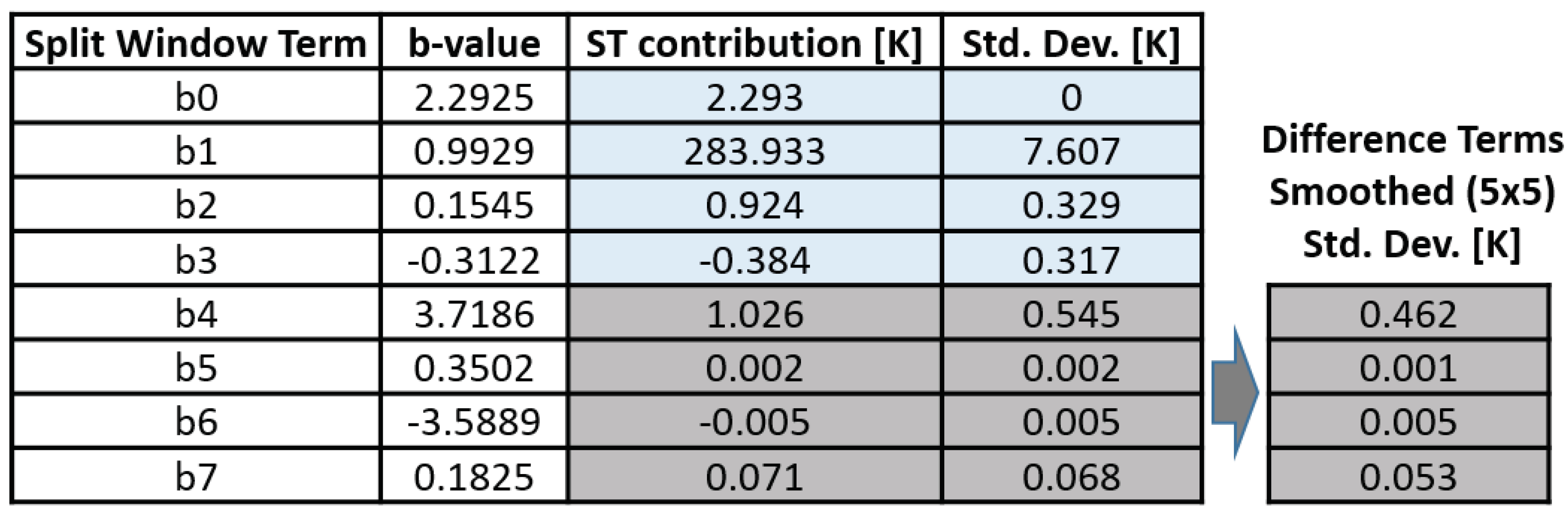
To motivate a potentially desirable solution, Figure 5 shows the contributions of each term in Equation (1) to the final surface temperature product for the scene in Figure 3. Columns 3 and 4 of this table were populated by calculating the scene-wide mean and standard deviation, respectively, of each term in Equation (1). Accordingly, column 3 represents the average magnitude of each term’s contribution to the final ST product, while column 4 represents the spatial variability introduced by each term to the final ST product. Note from the values in columns 3 and 4 that the additive terms in Equation (1) (highlighted in blue) contribute most of the overall magnitude and variability to the final ST product for the scene in Figure 3. Conversely, note from the values in columns 3 and 4 that the difference terms from Equation (1) (highlighted in gray) contribute significantly less information to the final product. Since the difference terms introduce the artifacts shown in Figure 3, and their radiometric contribution to the final product is relatively small, a proposed solution to mitigate these artifacts is to apply a 5 × 5 smoothing filter to the Band 10 and 11 apparent temperature images for terms b₄ through b₇ in Equation (1). Recall that the TIRS nominal ground sampling distance is approximately 100 m, but the calculated full width at half maximum (FWHM) of its point-spread function is approximately 200 m (see Wenny et al., 2015) [27]. Therefore, averaging the upsampled 30 m data to 150 m will not significantly alter the image data collected by TIRS. Comparing the nominal standard deviations for the b₄ through b₇ terms (column 4: gray terms) to the 5 × 5 smoothed standard deviations, as suggested here (zoomed: gray terms), smoothing has a negligible impact (less than 0.1 K) on the scene-wide variability observed in the final proposed ST product for the scene in Figure 3.

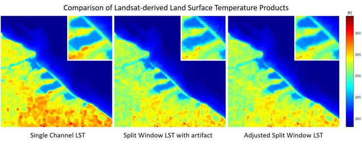
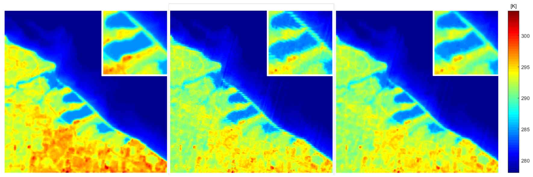
While smoothing the difference terms in Equation (1) appears to have negligible impact on radiometric fidelity, its effect on mitigating the geometric artifacts in Figure 3 is dramatic. Figure 6 shows the single channel ST product (left), the nominal split window ST product (middle), and the proposed split window ST product (right). Note that the single channel product is presented here for reference, as it should not exhibit the artifacts described in this section. By visually inspecting the zoom windows in Figure 6, the artifacts present in the nominal split window product (middle) are essentially removed with the proposed methodology (right).

3. Results and Validation

The 1518 Landsat 8 scenes corresponding to the ground reference sites listed in Table 2 were processed to surface temperature using the proposed split window method and the coefficients described here (see Table 1). The difference between the derived ST and the measured (reference) ST is shown in Figure 7 for all reference sites. Note that the difference data is displayed as a function of “distance to the nearest cloud (km)” from the pixel where the comparison is made to a reference measurement. As seen in the figure, the temperature error is greatest when the target pixel is in close proximity to a cloud, which adds significant uncertainty to the ST retrieval process. The mean error for the data in Figure 7 is 0.2 K with a standard deviation of 2.73 K. However, ignoring data points within 4 km of a cloud, the mean error becomes 0.02 K with a standard deviation of 1.39 K.

Surface temperature products using the single channel methodology and the split window algorithm with the coefficients reported in Du et al. (2015) were also calculated to serve as a comparison to the proposed method. The results from the three methods can be summarized in Figure 8, which shows the average differences between the reference temperature measurements and the Landsat-derived surface temperatures (left), and the corresponding standard deviations of the residuals (right) as functions of distance to cloud.

In general, for the full set of data compiled in this study, the proposed split window implementation (blue bars) has better accuracy and precision than the other two algorithms, as compared to reference data. Figure 8 (left) shows that its retrieved temperatures are, on average, closer to reference measurements with a slight positive bias that diminishes as distance to the nearest cloud increases. Notice that the single channel methodology has a significant bias (compared to reference measurements), which is consistent with the temperature products shown in Figure 3 and Figure 6. Figure 8 (right) indicates that the residuals about the mean are smaller for the proposed split window implementation regardless of cloud proximity for the implementation proposed here.

Two interesting observations can be made when categorizing the data in Figure 8 into “land sites” and “water sites”. Figure 9 (left) shows the mean difference between derived and measured surface temperatures for the “land sites” while Figure 9 (right) shows the corresponding standard deviations of the residuals about the mean. The first noteworthy observation from Figure 9 (right) is that for relatively clear scenes (i.e., clouds are over five kilometers from the ground reference measurement), all three methodologies show a standard deviation of approximately 2 K, compared to surface measurements. These values are consistent with those observed in studies using SURFRAD as a reference for validation of other spaceborne thermal instruments [28,29,30]. Given that this 2 K residual error is consistently observed from several spaceborne platforms and that the pyrgeometers used at the land-based reference sites are sensitive from 4 to 50 μm, this residual error indicates that reflected solar radiation may be contributing to the signal recorded by the pyrgeometers and that broadband emissivity uncertainty is potentially a limiting factor in leveraging these sites to be used as reference sources for applications requiring high accuracy.

A second observation can be made by referring to Figure 10. Figure 10 (left) shows the mean difference between derived and measured surface temperatures for the “water sites”, while Figure 10 (right) shows the corresponding standard deviation of the residuals about the mean. The blue bars indicate that the split window algorithm (as presented here) estimates surface temperature more accurately and with less residual error than the single channel method (red bars) and the split window algorithm using the coefficients presented in Du et al. (2015) (gray bars). The under-performance of the Du et al. coefficients for retrieving water temperature is likely due to the inclusion of man-made materials into their training process; i.e., the algorithm coefficients are over-fit to land-based targets. This outcome highlights the potential necessity to develop material-based b-coefficients for an operational split window implementation.

4. Conclusions

The TIRS instruments onboard Landsats 8 and 9 contain two thermal channels, enabling the use of the split window methodology to derive Earth surface temperature. This work focused on tailoring the generalized split window algorithm to the specific Landsat bands by deriving appropriate algorithm coefficients and by addressing the inherent aliasing artifacts in the split window temperature product. For the scenes tested here, validation efforts illustrate that the split window ST product is more accurate than the single channel ST product (available in the Landsat Collection 2 release).

The studies presented here demonstrate that smoothing the difference terms in Equation (1) has a dramatic effect on mitigating aliasing artifacts introduced by band-to-band misregistration and upsampling of the nominal TIRS image data. Several comparisons (analogous to Figure 5 in Section 2.4) of the unsmoothed to the smoothed 30 m temperature product indicate that smoothing has little impact on in-scene variability. Considering the fact that the TIRS nominal ground sampling distance is approximately 100 m and the calculated FWHM of its point-spread function is approximately 200 m [27], the solution presented here is believed to be appropriate, although quantifying the impact of smoothing remains an area of ongoing research.

From a radiometric viewpoint, Figure 10 highlights the potential value of deriving per-material split window coefficients for an operational implementation. Considering Du et al. tuned their split window coefficients to support urban heat island applications, the under-performance of their implementation for the water scenes tested here precludes their coefficients from being used for environmental applications requiring less than one Kelvin precision. That being said, the simulated effort conducted by Du et al. highlights potential improvements that can be made to surface temperature retrieval if atmospheric water vapor can be characterized from image data and accounted for in the split window implementation; i.e., the b-coefficients in Equation (1) are categorized as a function of column water vapor. An investigation into the potential improvement of surface temperature estimation using coefficients categorized by material and column water vapor will be conducted.

Other considerations to achieve an operational implementation and validation of a split window algorithm for TIRS in Collection 3 are the development of a quality assurance map and appropriate validation of the product. The single channel algorithm being implemented in Collection 2 to derive surface temperature for the Landsat thermal archive contains a quality assurance (QA) band that was developed based on cloud proximity and atmospheric transmission [2]. While this QA band will provide information regarding the product’s accuracy, it is highly dependent on Landsat’s cloud mask and was trained using water observations. The investigation and development of an analogous but appropriately-trained quality assurance band to accompany a split window-derived surface temperature product represents an area of ongoing research.

While the efforts reported here represent significant progress toward the development and validation of an operational split window-derived surface temperature product, the considerations described above should be addressed before the final form of the algorithm is achieved. Future validation efforts will include reprocessing of the scenes presented here but with Collection 2 L1T TIRS data, incorporation of additional reference measurements as they become available, and a categorization of the residual errors with a more appropriate metric; i.e., residual errors between retrieved and reference measurements will be categorized as a function of atmospheric column water vapor instead of distance to cloud.

References

1. Malakar, N.; Hulley, G.; Hook, S.; Laraby, K.; Cook, M.; Schott, J. An Operational Land Surface Temperature Product for Landsat Thermal Data: Methodology and Validation. IEEE Trans. Geosci. Remote Sens. 2018, 56, 5717–5735. [Google Scholar] [CrossRef]
2. Laraby, K.G.; Schott, J.R. Uncertainty estimation method and Landsat 7 global validation for the Landsat surface temperature product. Remote Sens. Environ. 2018, 216, 472–481. [Google Scholar] [CrossRef]
3. Reuter, D.; Richardson, C.; Pellerano, F.; Irons, J.; Allen, R.; Anderson, M.; Jhabvala, M.; Lunsford, A.; Montanaro, M.; Smith, R.; et al. The Thermal Infrared Sensor (TIRS) on Landsat 8: Design Overview and Pre-Launch Characterization. Remote Sens. 2015, 7, 1135–1153. [Google Scholar] [CrossRef] [Green Version]
4. Gerace, A.; Montanaro, M. Derivation and validation of the stray light correction algorithm for the Thermal Infrared Sensor onboard Landsat 8. Remote Sens. Environ. 2017, 191, 246–257. [Google Scholar] [CrossRef]
5. Storey, J.; Choate, M.; Moe, D. Landsat 8 Thermal Infrared Sensor Geometric Characterization and Calibration. Remote Sens. 2014, 6, 11153–11181. [Google Scholar] [CrossRef] [Green Version]
6. Becker, F.; Li, Z.L. Towards a local split window method over land surfaces. Int. J. Remote Sens. 1990, 11, 369–393. [Google Scholar] [CrossRef]
7. Wan, Z.; Dozier, J. A generalized split-window algorithm for retrieving land-surface temperature from space. IEEE Trans. Geosci. Remote Sens. 1996, 34, 892–905. [Google Scholar] [CrossRef] [Green Version]
8. Wan, Z. New Refinements and Validation of the MODIS Land-Surface Temperature/Emissivity Products. Remote Sens. Environ. 2008, 140, 59–74. [Google Scholar] [CrossRef]
9. Berk, A.; Conforti, P.; Kennett, R.; Perkins, T.; Hawes, F.; van den Bosch, J. MODTRAN6: A major upgrade of the MODTRAN radiative transfer code. In Proceedings of the 2014 6th Workshop on Hyperspectral Image and Signal Processing: Evolution in Remote Sensing (WHISPERS), Lausanne, Switzerland, 24–27 June 2014; pp. 113–119. [Google Scholar] [CrossRef]
10. Thermodynamic Initial Guess Retrieval (TIGR). Available online: http://ara.abct.lmd.polytechnique.fr/index.php?page=tigr (accessed on 22 October 2019).
11. MODIS UCSB Emissivity Library. Available online: https://icess.eri.ucsb.edu/modis/EMIS/html/em.html (accessed on 22 October 2019).
12. Du, C.; Huazhong, R.; Qin, Q.; Meng, J.; Zhao, S. A Practical Split-Window Algorithm for Estimating Land Surface Temperature from Landsat 8 Data. Remote Sens. 2015, 7, 647–665. [Google Scholar] [CrossRef] [Green Version]
13. Hulley, G.C.; Hook, S.J.; Abbott, E.; Malakar, N.; Islam, T.; Abrams, M. The ASTER Global Emissivity Dataset (ASTER GED): Mapping Earth’s emissivity at 100 meter spatial scale. Geophys. Res. Lett. 2015, 42, 7966–7976. [Google Scholar] [CrossRef]
14. Sibandze, P.; Mhangara, P.; Odindi, J.; Kganyago, M. A comparison of Normalised Difference Snow Index (NDSI) and Normalised Difference Principal Component Snow Index (NDPCSI) techniques in distinguishing snow from related land cover types. S. Afr. J. Geomat. 2014, 3, 197–209. [Google Scholar] [CrossRef] [Green Version]
15. SURFRAD (Surface Radiation Budget) Network. Available online: https://www.esrl.noaa.gov/gmd/grad/surfrad/ (accessed on 22 October 2019).
16. AmeriFlux Network. Available online: https://ameriflux.lbl.gov/ (accessed on 22 October 2019).
17. National Data Buoy Center. Available online: https://www.ndbc.noaa.gov/ (accessed on 22 October 2019).
18. Lake Tahoe Validation. Available online: https://laketahoe.jpl.nasa.gov/get_met_weather (accessed on 22 October 2019).
19. Salton Sea Validation. Available online: https://saltonsea.jpl.nasa.gov/get_met_weather (accessed on 22 October 2019).
20. Wang, K.; Dickinson, R.E. Global atmospheric downward longwave radiation at the surface from ground-based observations, satellite retrievals, and reanalyses. Rev. Geophys. 2013, 51, 150–185. [Google Scholar] [CrossRef]
21. Guillevic, P.C.; Privette, J.L.; Coudert, B.; Palecki, M.A.; Demarty, J.; Ottle, C.; Augustine, J.A. Land Surface Temperature product validation using NOAA’s surface climate observation networks—Scaling methodology for the Visible Infrared Imager Radiometer Suite (VIIRS). Remote Sens. Environ. 2012, 124, 282–298. [Google Scholar] [CrossRef] [Green Version]
22. University of Michigan Biological Station. Available online: http://flux.org.ohio-state.edu/site-description-umbs/#umbs-ameriflux-towers (accessed on 22 October 2019).
23. Gröbner, J.; Wacker, S. Pyrgeometer Calibration Procedure at the PMOD/WRC-IRS. Davos:[sn]. 2012. Available online: https://library.wmo.int/doc_num.php?explnum_id=7365 (accessed on 8 January 2020).
24. Wang, K.; Wan, Z.; Wang, P.; Sparrow, M.; Liu, J.; Zhou, X.; Haginoya, S. Estimation of surface long wave radiation and broadband emissivity using Moderate Resolution Imaging Spectroradiometer (MODIS) land surface temperature/emissivity products. J. Geophys. Res. Atmos. 2005, 110. [Google Scholar] [CrossRef]
25. Masuda, K.; Takashima, T.; Takayama, Y. Emissivity of pure and sea waters for the model sea surface in the infrared window regions. Remote Sens. Environ. 1988, 24, 313–329. [Google Scholar] [CrossRef]
26. Zeng, X.; Zhao, M.; Dickinson, R.E.; He, Y. A multiyear hourly sea surface skin temperature data set derived from the TOGA TAO bulk temperature and wind speed over the tropical Pacific. J. Geophys. Res. Oceans 1999, 104, 1525–1536. [Google Scholar] [CrossRef]
27. Wenny, B.; Helder, D.; Hong, J.; Leigh, L.; Thome, K.; Reuter, D. Pre- and Post-Launch Spatial Quality of the Landsat 8 Thermal Infrared Sensor. Remote Sens. 2015, 7, 1962–1980. [Google Scholar] [CrossRef] [Green Version]
28. Yu, Y.; Tarpley, D.; Privette, J.L.; Flynn, L.E.; Xu, H.; Chen, M.; Vinnikov, K.Y.; Sun, D.; Tian, Y. Validation of GOES-R Satellite Land Surface Temperature Algorithm Using SURFRAD Ground Measurements and Statistical Estimates of Error Properties. IEEE Trans. Geosci. Remote Sens. 2012, 50, 704–713. [Google Scholar] [CrossRef]
29. Li, S.; Yu, Y.; Sun, D.; Tarpley, D.; Zhan, X.; Chiu, L. Evaluation of 10 year AQUA/MODIS land surface temperature with SURFRAD observations. Int. J. Remote Sens. 2014, 35, 830–856. [Google Scholar] [CrossRef]
30. Liu, Y.; Yu, Y.; Yu, P.; Göttsche, F.M.; Trigo, I. Quality assessment of S-NPP VIIRS land surface temperature product. Remote Sens. 2015, 7, 12215–12241. [Google Scholar] [CrossRef] [Green Version]
Figure 1. Process flow to derive split window coefficients by propagating modeled surface temperatures, emissivities, and atmospheric conditions to the top of atmosphere and regressing the band-effective apparent temperatures against the known input surface temperatures.
Remotesensing 12 00224 g001
Figure 2. TIGR atmospheric profiles for various atmospheric types compared to MODTRAN’s default atmospheres. The black data curves are air temperatures as a function of altitude, while the red data curves are the associated dew point temperatures.
Remotesensing 12 00224 g002
Figure 3. Comparison of the surface temperature product derived from the single channel method (left) against the split window method (right) for an area around Lake Ontario, NY (Landsat scene ID: LC08_L1TP_016030_20190413_20190422_01_T1). Note the spatial artifacts along edges in the split window product. Zoom windows are shown in the upper right of each image. The image area is roughly 8 by 8 km, and north is up.
Remotesensing 12 00224 g003
Figure 4. The Thermal Infrared Sensor (TIRS) focal plane array consists of three detector arrays (labeled A, B, and C) arranged to span the cross-track 185 km swath. Spectral filters over the arrays produce the two thermal bands (Bands 10 and 11).
Remotesensing 12 00224 g004
Figure 5. Table illustrating the contribution of each term from Equation (1) to the final surface temperature product shown in Figure 3. Columns 3 and 4 of this table were populated by calculating the scene-wide mean and standard deviation, respectively, of each term in Equation (1). Note that the additive terms (highlighted in blue) contribute most of the overall magnitude (column 3) and variability (column 4) to the final ST product. When compared to the difference terms in column 4 (highlighted in gray), the zoom window suggests that smoothing the difference terms has little impact on scene-wide variability.
Remotesensing 12 00224 g005
Figure 6. Comparison of surface temperature products: single channel product (left), the nominal split window product (middle), and the proposed split window product (right) (Landsat scene ID: LC08_L1TP_016030_20190413_20190422_01_T1). The scene is roughly 8 by 8 km, and north is up.
Remotesensing 12 00224 g006
Figure 7. The difference between the reference temperature measurements and the Landsat-derived surface temperatures for the proposed split window methodology as a function of distance to nearest cloud.
Remotesensing 12 00224 g007
Figure 8. All sites validation: the average differences between the reference temperature measurements and the Landsat-derived surface temperatures for the three retrieval methodologies (left) and the corresponding standard deviations of the residuals (right).
Remotesensing 12 00224 g008
Figure 9. Results over land sites: the average differences between the reference temperature measurements and the Landsat-derived surface temperatures for the three retrieval methodologies (left), and the corresponding standard deviations of the residuals (right).
Remotesensing 12 00224 g009
Figure 10. Results over water sites: the average differences between the reference temperature measurements and the Landsat-derived surface temperatures for the three retrieval methodologies (left), and the corresponding standard deviations of the residuals (right). Note that there is no reference data for clouds within 0–1 km of a water buoy.
Remotesensing 12 00224 g010