A Geographically Weighted Regression Approach to Understanding Urbanization Impacts on Urban Warming and Cooling: A Case Study of Las Vegas

Abstract

A surface urban heat island (SUHI) effect is one of the most significant consequences of urbanization. Great progress has been made in evaluating the SUHI with cross-sectional studies performed in a number of cities across the globe. Few studies; however, have focused on the spatiotemporal changes in an area over a long period of time. Using multi-temporal remote sensing data sets, this study examined the spatiotemporal changes of the SUHI intensity in Las Vegas, Nevada, over a 15-year period from 2001 to 2016. We applied the geographically weighted regression (GWR) and advanced statistical approaches to investigating the SUHI variation in relation to several important biophysical indicators in the region. The results show that (1) Las Vegas had experienced a significant increase in the SUHI over the 15 years, (2) Vegetation and large and small water bodies in the city can help mitigate the SUHI effect and the cooling effect of vegetation had increased continuously from 2001 to 2016, (3) An urban heat sink (UHS) was identified in developed areas with low to moderate intensity, and (4) Increased surface temperatures were mainly driven by the urbanization-induced land conversions occurred over the 15 years. Findings from this study will inspire thoughts on practical guidelines for SUHI mitigation in a fast-growing desert city.

1. Introduction

An urban heat island (UHI) phenomenon refers to raised temperatures in urban areas in comparison to the surrounding rural areas [1]. This phenomenon results from the replacement of natural landscape components with manmade features, which detrimentally affect socio-ecological functioning and services well beyond city boundaries [2]. Severe UHI effects lead to higher energy and water demand for cooling [3], degradation of urban air quality [4], decreased human thermal comfort [5], and, more importantly, increased risk of heat-related mobility and mortality especially for the elderly and children [6]. Well-known UHI mitigation methods include the redevelopment and optimally arrangement of urban green and blue infrastructure (e.g., trees/lawns, urban parks, urban lakes) [7,8,9,10], deployment of green/white roofs [11,12], and the better design of urban wind corridor to increase ventilation [13].

Traditionally, UHI studies were conducted using air temperature loggers from in situ monitoring stations [14]. Although the in situ monitoring stations can capture long and continuous data records in high temporal resolution, it suffers from the sparsely distributed data with limited spatial coverage [15]. With the advancement of thermal remote sensing, researchers have been able to obtain thermal remotely sensed images with higher levels of spatial and temporal resolution [16]. Available satellite thermal remote sensing sensors include National Oceanic and Atmospheric Administration (NOAA) (Advanced Very-High-Resolution Radiometer (AVHRR)), Earth Observing System (EOS) (Moderate Resolution Imaging Spectroradiometer (MODIS), Advanced Spaceborne Thermal Emission and Reflection Radiometer (ASTER)), and Landsat (Thematic Mapper (TM), Enhanced Thematic Mapper Plus (ETM+), Operational Land Imager (OLI)/Thermal Infrared Sensor (TIRS)), which offer an excellent opportunity for studying the surface urban heat island (SUHI) effect in relation to a variety of environmental, ecological, and socio-economic parameters at a much larger spatial scale.

The land surface temperature (LST) in urban areas is closely linked to human-induced land use land cover (LULC) transformation [2,17,18]. For instance, researchers found the LST to be negatively associated with the abundance of urban greenspace and positively associated with the density of impervious surfaces [19,20,21,22]. More research has confirmed the relationship of the LST with other land cover features. For example, Chen et al. found a negative relationship between water bodies and daytime surface temperatures in a study of Shenzhen, China [23]. Wang et al. identified a significantly positive relationship of the daytime LST with open soil and fallow cropland over the Phoenix metropolitan area [24].

Many existing studies have used the ordinary least squares (OLS) regression to understand the underlying relationships between the LST and land cover composition [24,25,26]. For example, Yuan and Bauer used the OLS to study the relationship between the LST and percent impervious surfaces in the metropolitan area of Minneapolis–Saint Paul, Minnesota [22]. In another study, Zhou et al. evaluated the variation in the SUHI in relation to a number of environmental parameters using correlation analysis and simple linear regression [25]. In spite of the number of variables being considered, these studies only focused on the bivariate relationships without considering the confounding effect from other variables. Using multiple linear regression analysis, Wang et al. examined the zonal and temporal variations in the SUHI with respect to several land cover variables over the Phoenix metropolitan area [24]. Despite the popularity and wide adoption of the OLS regression in the existing research, it fails to consider the spatial dependence and spatial heterogeneity with the assumption of a constant process throughout the study area. In reality, however, the processes driving the spatial phenomenon vary from place to place, and there is a higher degree of association among closer observations than distant ones [27].

Many advanced spatial statistics methods have been developed to address the spatial heterogeneity issues, including spatial econometrics/regression [28], the geographically weighted regression (GWR) [29,30], and spatial filtering techniques [31]. Much existing research has used the GWR to understand the potential relationships between LST and land cover composition in different parts of the globe [26,32,33]. While the spatial variations have been effectively addressed and represented with the use of GWR, temporal changes of urban areas have been largely overlooked by most studies. The goal of this research is to fill this knowledge gap by offering a longitudinal study that permits a spatiotemporal evaluation of the SUHI intensity. Coupling remote sensing and advanced spatial statistical modeling, this study aims to achieve the following objectives: (1) examining the spatial distribution and temporal changes of the SUHI over a 15-year time period; (2) evaluating the spatiotemporal relationships between the SUHI and a number of biophysical variables using correlation analysis and GWR; and (3) suggesting proper heat mitigation and adaption strategies through analyzing the urbanization impacts on urban warming.

2. Materials and Methods

2.1. Study Area

Our study area is the city of Las Vegas, a subtropical desert city located within the greater Mojave Desert (Figure 1). As the most populous city in Nevada, Las Vegas has experienced a fast-urban expansion with an average area increase of 40 km² per year from 1990 to 2010 [2]. The population in Las Vegas has grown significantly since the 1960s with an average increasing rate of 85.2% from 1990 to 2000. The estimated population in 2018 was 648,224 million [34]. The rapid growth is largely driven by the role of the city as a cultural, financial, and recreational center in Nevada. The average daytime temperature in June is 41 °C, with the maximum temperature reaching 45 °C [35]. On average, there are 310 sunny days per year, and the average rainfall is only 2.8 mm [35]. Las Vegas experienced the most intense UHI effects in 2016, with a 4 ℃ temperature difference between its metropolitan area and the surrounding rural area [36].

2.2. SUHI Intensity Derivation

Three Landsat 5 Thematic Mapper (TM) images and one Landsat 8 Operational Land Imager (OLI) image were obtained from the USGS EarthExplorer website [37]. The acquisition dates are July 13th, 2001, July 31st, 2006, July 17th, 2011, and July 26th, 2016, respectively. The thermal bands were used to retrieve the LST over Las Vegas in these four years. The wavelength and spatial resolution of the thermal band are 10.4–12.5 µm and 120 meters for Landsat 5 TM, and 10.6–11.19 µm and 100 meters for Landsat 8 OLI image [38].

We applied the mono-window algorithm to retrieving the LST [39]. First, the thermal band was used to calculate the brightness temperature, ${\mathrm{T}}_6$ (Equation (1)).

$${\mathrm{T}}_6=\frac{1260.56}{\ln \left[1+\frac{60.776}{0.1238+0.00563256{\ast \mathrm{DN}}_{\mathrm{b}6}}\right]}$$

(1)

where ${\mathrm{T}}_6$ is the brightness temperature (Unit: Kelvin). ${\mathrm{DN}}_{\mathrm{b}6}$ is the digital number (DN) value of the thermal band. Next, the brightness temperature was converted into the LST following Equation (2).

$${\mathrm{T}}_{\mathrm{s}}=\frac{\left\{67.3554\left(\mathrm{C}+\mathrm{D}-1\right)+\left[0.4414\left(\mathrm{C}+\mathrm{D}\right)+0.4586\right]{\ast \mathrm{T}}_6-\mathrm{D}\ast \mathrm{K}\right\}}{\mathrm{C}}$$

(2)

where ${\mathrm{T}}_{\mathrm{s}}$ is the derived LST with the unit of Kelvin. K is the mean air temperature on the day of acquisition sourced from the National Oceanic and Atmospheric Administration (NOAA) [35]. C and D are intermediate variables given by Equations (3) and (4).

$$\mathrm{C}={\mathsf{\epsilon }\mathsf{\tau }}_6$$

(3)

$$\mathrm{D}=\left(1-\mathsf{\epsilon }\right)\left[1+\left(1-\mathsf{\epsilon }\right){\mathsf{\tau }}_6\right]$$

(4)

where ${\mathsf{\tau }}_6$ is the atmospheric transmittance, and $\mathsf{\epsilon }$ is the land surface emissivity. The values of ${\mathsf{\tau }}_6$ and ε were obtained from the online NASA atmospheric correction parameter calculator [40]. The mono-window algorithm was implemented using the ENVI 5.0 software [41].

With the retrieved LST, the SUHI intensity is defined as the LST difference between the urban area and its surrounding rural area. The city boundary was sourced from the United States Census Bureau [34]. We created a buffer that is 10–20 km outside of the city boundary to avoid the transition zone between urban and rural areas. The buffer distance was determined based on several studies and a series of trial-and-error tests [2,24,42]. To minimize the confounding effects from areas with high elevation and water, mountains, and large water bodies within the buffer were manually removed. The SUHI intensity maps were created by subtracting the mean LST in the rural area from the LST value of each urban pixel.

2.3. Biophysical Indicators

We used biophysical indices to represent three major land cover features in the study area, including vegetation, built-up, and water body. The biophysical indices were calculated based on mathematical manipulation of spectral bands. The soil adjusted vegetation index (SAVI) was used to represent green biomass in the region (Equation (5)). The near-infrared (NIR) band and the red band were applied to the SAVI calculation. The SAVI was selected over the NDVI because it eliminates soil-induced variations in the NDVI, making it more effective for distinguishing green vegetation from open soil, particularly in semi-arid areas [43]. The normalized difference built-up index (NDBI) (Equation (6)) was used to identify the built-up area [44]. It was calculated by enhancing the mid-infrared band (MIR) while suppressing the near-infrared band. We used the modified normalized difference water index (MNDWI) to extract water bodies in the urban area (Equation (7)) [45]. The green band and the short-wave infrared (SWIR) band were applied to the MNDWI calculation. Water bodies extracted using the normalized difference water index (NDWI) are subject to overestimation due to the spectral mixture with built-up areas. The MNDWI is a modified version of the NDWI that successfully picks out water bodies from the surrounding built-up areas [46]. Given the high proportion of developed areas in Las Vegas, we believe that the MNDWI provides a more accurate estimation of water bodies than the NDWI.

$$\mathrm{SAVI}=\frac{\rho \left(NIR\right)-\rho \left(Red\right)}{\rho \left(NIR\right)-\rho \left(Red\right)+L}\left(1+L\right)$$

(5)

where L is a soil adjustment factor, L = 0.5

$$\mathrm{NDBI}=\frac{\rho \left(MIR\right)-\rho \left(NIR\right)}{\rho \left(MIR\right)+\rho \left(NIR\right)}$$

(6)

$$\mathrm{MNDWI}=\frac{\rho \left(Green\right)-\rho \left(SWIR\right)}{\rho \left(Green\right)+\rho \left(SWIR\right)}$$

(7)

2.4. Statistical Analysis

A total of 1000 randomly selected points was used as our sample points. The sample points were created using the ArcMap software [47], and they are identical for the four years.

Table 1. Descriptive statistics of the surface urban heat island (SUHI) intensity and biophysical variables for years 2001, 2006, 2011, and 2016.

	2001		2006		2011		2016
	Mean	StDev	Mean	StDev	Mean	StDev	Mean	StDev
SUHI	−1.11	3.19	−0.99	3.03	−0.12	2.80	1.12	3.03
SAVI	0.02	0.15	−0.01	0.14	0.00	0.14	0.14	0.10
NDBI	0.19	0.09	0.19	0.08	0.18	0.09	−0.02	0.06
MNDWI	−0.22	0.11	−0.04	0.10	−0.05	0.10	−0.04	0.07

shows the summary statistics of the SUHI and biophysical variables based on all sample points in the study region. The mean SUHI intensity based on the sample points increased from −1.11 °C in 2001 to 1.12 °C in 2016, indicating a continuous increase in the average SUHI over the 15 years.

We performed a correlation analysis to understand the bivariate relationships between the SUHI and the biophysical indicators. A multiple regression analysis was later conducted to evaluate the individual contribution of each biophysical variable to the SUHI while controlling for the effects of other variables.

The GWR was performed to understand local variations and to be able to visualize the local relationships spatially [48,49,50]. Mathematically, the GWR is given by:

$$y_i={\beta }_0\left(u_i,v_i\right)+{\displaystyle \sum }_{j=1}{\beta }_j\left(u_i,v_i\right)x_{ij}+{\epsilon }_i$$

(8)

where $y_i$ is the dependent variable, $x_{ij}$ is the jth independent variable at location i, and ${\epsilon }_i$ is a random error term at location $i$. $\left(u_i,v_i\right)$ are the coordinates of the observed location i and ${\beta }_j\left(u_i,v_i\right)$ is the coefficient associated with the jth variable at location i.

The kernel and bandwidth are key parameters in the GWR model that affect model accuracy. We used the adaptive Gaussian kernel because the sampling points were randomly distributed over an irregular study area. The optimal bandwidth was determined following the golden search algorithm. The model accuracy was evaluated using the corrected Akaike Information Criterion (AICc) [48]. Lower values of AICc indicate a better model fit. The GWR models were estimated using the GWR 4.0 [51].

2.5. Statistical Summary by LULC Type

Four LULC maps were created from the National Land Cover Dataset (NLCD) to understand the SUHI changes in the context of urbanization in Las Vegas (Figure 2). The NLCD provides nationwide land cover products for the United States with a 30-meter resolution [52]. Nine LULC types were extracted for the region, including developed open space, developed low intensity, developed medium intensity, developed high intensity, barren land (rock/sand/clay), shrub/scrub, open water, grassland/herbaceous, and woody wetlands.

For each LULC type, we summarized the local estimates for the three biophysical indicators and evaluated the SUHI changes in the context of rapid urbanization. The ability to generate localized estimates and observing them under a particular regionalization scheme are distinct advantages of local models like the GWR. Understanding how the relationships evolve over time will shed light on better management of natural resources and the smart growth of a desert city.

3. Results

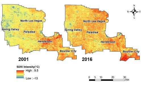
3.1. SUHI Intensity Maps

Figure 3 shows the spatial distribution of the SUHI over Las Vegas for the four years observed. In 2001, there was an increasing trend in the SUHI from northwest to southeast of the region, with the hottest area observed in the city of Henderson. Over the 15-year study period, there was a significant expansion of areas with warm temperatures. By 2016, the heat island effect had greatly intensified for the region. The average SUHI was −1.083°C in 2001 compared with 1.187 °C in 2016 for the entire study area, a 2.27 °C increase. Areas experiencing the most temperature increases include the Las Vegas Strip, downtown Las Vegas, and the Boulder city at the southeast corner. For example, the mean SUHI in downtown Las Vegas changed from 0.467 °C in 2001 to 3.013 °C in 2016. Overall, there was a consistent increase in the SUHI across Las Vegas, with only a couple of negative SUHI pockets in 2016.

3.2. Correlation Analysis

Table 2. Pearson’s r between the SUHI and biophysical indicators.

		SAVI	NDBI	MNDWI
SUHI	2001	−0.253 **	0.191 **	0.091 **
	2006	−0.364 **	0.290 **	−0.152 **
	2011	−0.247 **	0.250 **	−0.159 **
	2016	−0.484 **	0.500 **	−0.285 **

** Correlation is significant at the 0.01 level (p < 0.01).

shows the Pearson’s correlation between the SUHI and the biophysical indicators. For all years, the SUHI was significantly correlated with all the variables at the 0.01 level. There was a negative correlation between the SUHI and SAVI, and a positive correlation between the SUHI and NDBI. For both indices, the strongest relationships were observed in 2016. A weak, albeit significant correlation existed between the SUHI and MNDWI in 2001. It turned into a negative correlation and became stronger in the subsequent years.

3.3. Regression Analysis

Table 3. Summary of parameter estimates and diagnostics for the linear regression and geographically weighted regression (GWR) for 2001, 2006, 2011, and 2016.

2001	Linear regression				GWR
	β	S.E. a	p-value	VIF	Mean β b	S.D. c
SAVI	−1.85	1.34	0.167	4.12	−5.92	16
NDBI	6.78	2.3	0.003	4.8	−0.56	26.23
MNDWI	4.71	1.5	0.002	2.65	−.28	15.91
Diagnostics
AICc		4992.78			4203.26
Adjusted R2		0.07			0.618
Bandwidth		1000			75.77
2006	Linear regression				GWR
	β	S.E. a	p-value	VIF	Mean β b	S.D. c
SAVI	−8.72	1.33	<0.001	3.75	−6.83	9.2
NDBI	−1.96	3.56	0.038	9.59	4.93	19.51
MNDWI	−7.64	2.54	<0.001	6.43	−0.33	13.82
Diagnostics
AICc		5046.54			4400.50
Adjusted R2		0.156			0.607
Bandwidth		1000			68.22
2011	Linear regression				GWR
	β	S.E. a	p-value	VIF	Mean β b	S.D. c
SAVI	−3.98	1.16	<0.001	3.92	−5.15	9.37
NDBI	6.03	2.93	0.623	9.25	1.61	20.02
MNDWI	3.6	2.14	0.016	5.92	1.51	16.29
Diagnostics
AICc		4654.97			4063.12
Adjusted R2		0.100			0.557
Bandwidth		1000			69.93
2016	Linear regression				GWR
	β	S.E. a	p-value	VIF	Mean β b	S.D. c
SAVI	−12.32	1.62	<0.001	4.43	−11.41	15.26
NDBI	4.31	3.71	0.247	8.8	1.93	24.129
MNDWI	−8.66	2.66	0.001	5.15	−2.11	17.48
Diagnostics
AICc		4648.89			4076.65
Adjusted R2		0.3			0.665
Bandwidth		1000			52.77

^a S.E. is the standard error of the global parameter estimates; ^b Mean β is the averaged local estimates; ^c S.D. is the standard deviation of the local parameter estimates.

shows the regression results for the linear regression and GWR for the four years. There was no significant multicollinearity issue in the models based on the variance inflation factor (VIF). From the linear regression model, there was a negative relationship between the SUHI and SAVI, and the relationships were statistically significant for 2001, 2006, and 2011. The NDBI was positively related to the SUHI in 2001, which turned into negative in 2006, although the relationship was only marginally significant. The MNDWI was found to be significant for all years, but the direction of the relationship varied from year to year. A positive association was found in 2001 and 2011, and a negative association was observed in 2006 and 2016. The model failed to provide a very good fit for the data with an adjusted R2 ranging from 0.07 to 0.30. Overall, the results of the global linear regression were unstable and inconclusive, which calls for the need of a local estimation.

While the OLS creates global estimates for the entire region, the GWR generates a set of spatially varying estimates specific to a region defined by the local model. Table 3 lists the mean (Mean β) and standard deviation (S.D.) calculated based on all the local estimates. From the model diagnostics, the GWR achieved a significant improvement in model performance compared with the OLS, bringing the mean adjusted R² from 0.157 to 0.612. The averaged AICc for the OLS was 4835.8, which decreased to 4185.88 with the GWR. Local processes were identified by the GWR through much smaller bandwidths in models for all years, which represented very localized spatial relationships between SUHI intensity and biophysical parameters.

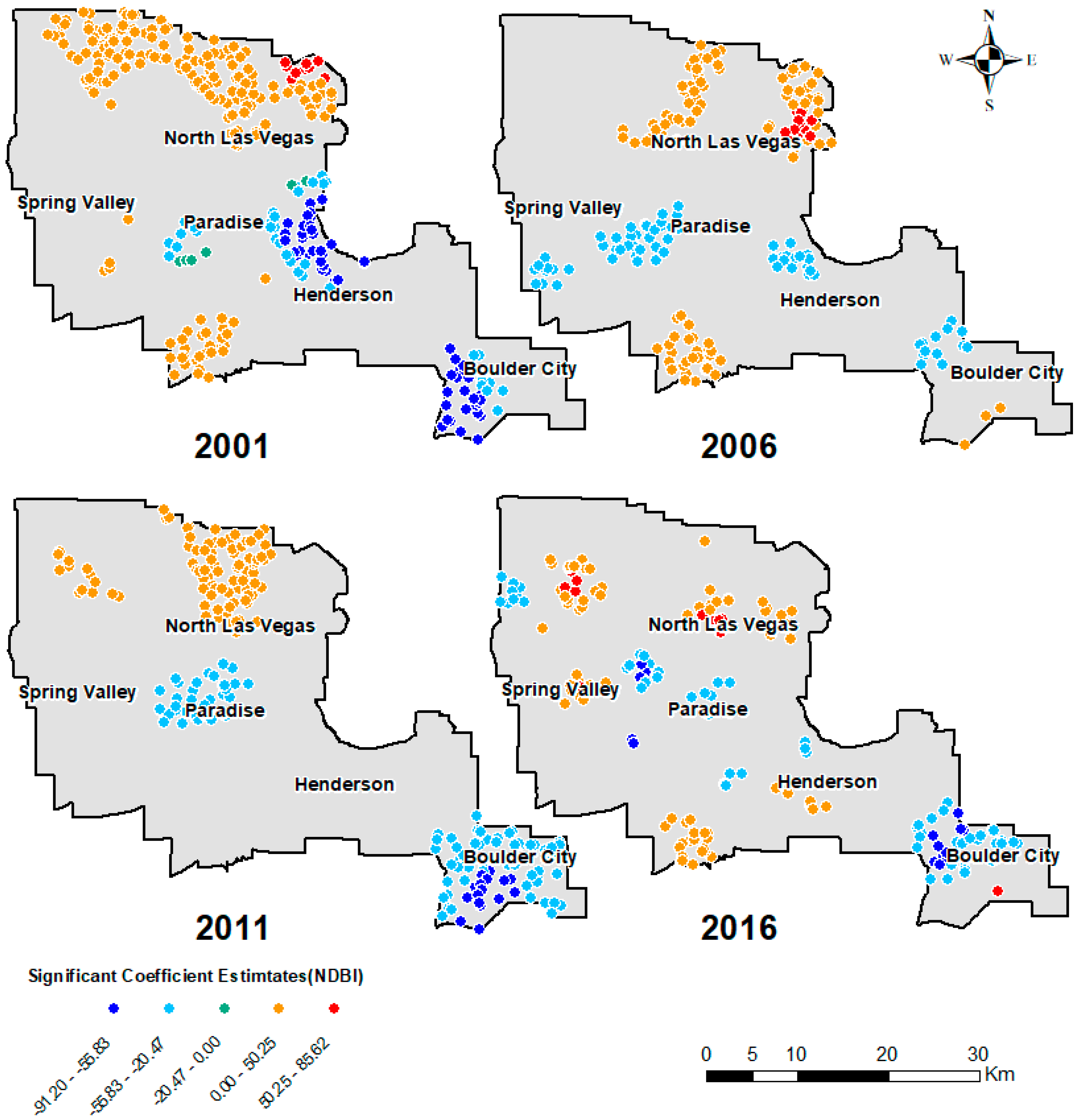
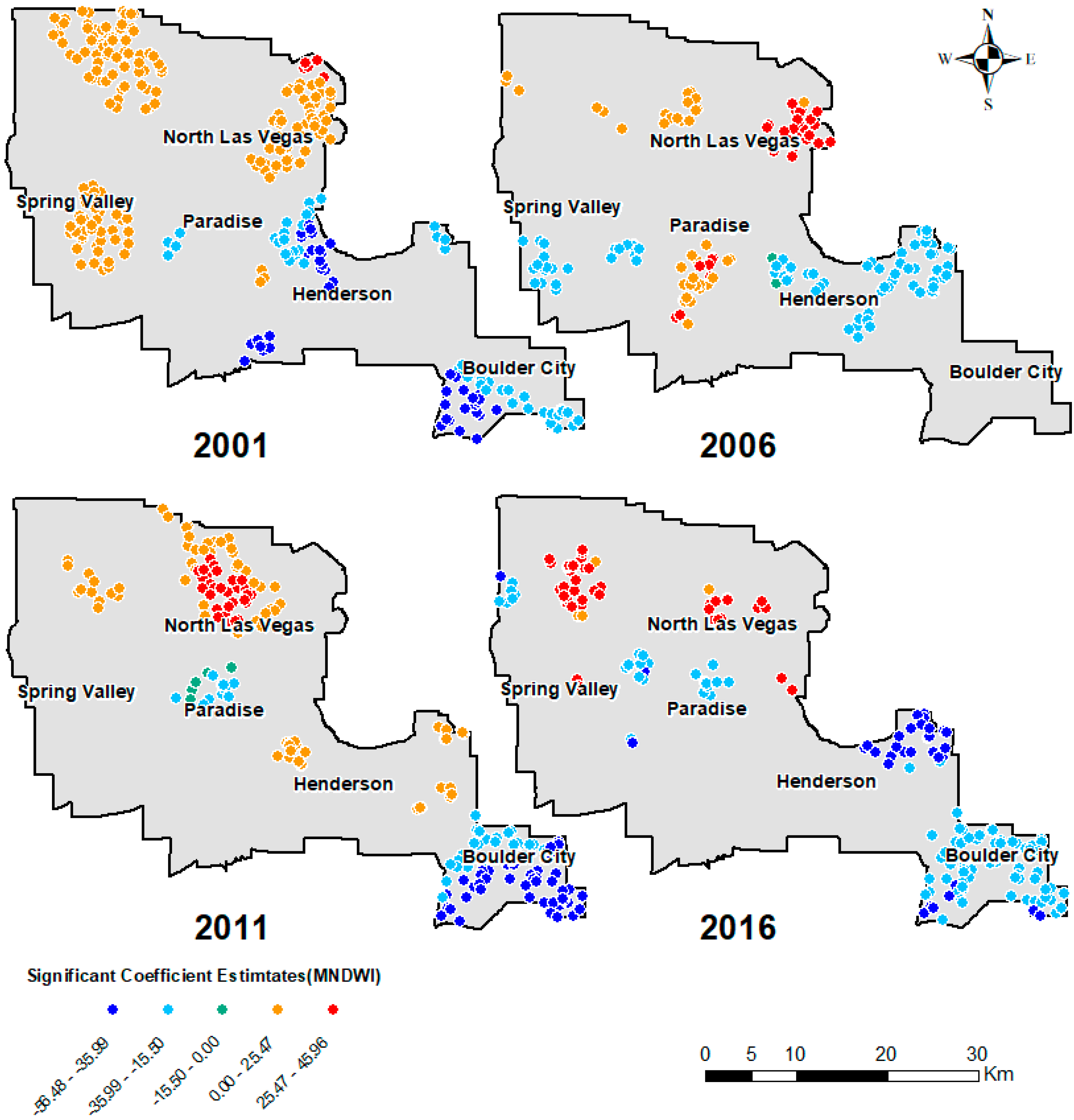
3.4. Spatial Patterns of the GWR Estimates

Figure 4, Figure 5 and Figure 6 show the locations and values of local estimates for the four years for SAVI, NDBI, and MNDWI, respectively. Only significant estimates were plotted (p < 0.05). From Figure 4, significant points were mostly found near Las Vegas Strip and Las Vegas downtown in all four years. Consistent with the correlation and global regression analysis, we found an intensifying relationship between the SAVI and SUHI intensity with more significant locations observed in 2016 than 2011. While only negative associations were found with global models, positive associations were identified for a few places in 2001, which turned non-significant or negative in the later years. The stronger relationship was not only supported by the increased number of significant locations, but also the size of the estimates. Two of the three clusters of positive places in 2001 disappeared in 2006, and the one located in Spring Valley turned into a negative cluster extending to the Strip in 2006 and 2011. The negative relationship continued to dominate the region, with a significant increase in both the number of places with negative estimates and the magnitude of the estimates.

A mix of positive and negative estimates was found in the relationship between the SUHI and NDBI (Figure 5). We observe significant positive associations in North Las Vegas in 2001, the area of which shrank gradually over the 15 years, leaving only a few clusters here and there in the region in 2016. Negative relationships were mainly found near the Strip and the Boulder City. While the intensity of positive and negative associations varied from year to year, the number of points with significant estimates had declined for both positive and negative relationships.

Figure 6 shows a combination of positive and negative relationships between the SUHI and MNDWI, with positive estimates in North Las Vegas and negative ones clustered in the middle and southeastern parts of the region. There was a decline in the number of positive estimates, while the number of negative estimates remained stable throughout the 15 years. Note that due to the low presence of the water body in the region, the estimates at non-water locations appeared to be spurious. Consistently negative estimates, however, were found near Lake Las Vegas and Boulder City.

3.5. Summarized Estimates by LULC Types

Table 4. Averaged coefficient estimates by land use land cover (LULC) type for 2001, 2006, 2011, and 2016.

	2001		2006		2011		2016
	SAVI	NDBI	SAVI	NDBI	SAVI	NDBI	SAVI	NDBI
Open Space	−4.34	2.92	−17.98	38.03	−11.65	10.67	−20.57	16.86
Low Intensity	−6.08	0.70	−17.53	12.13	−11.70	9.32	−21.97	7.04
Medium Intensity	−10.27	−12.83	−17.68	12.55	−13.23	−5.35	−20.55	12.58
High Intensity	−11.02	−17.57	−17.20	−11.98	−11.59	−5.45	−21.20	−2.74
Barren Land	−0.18	15.62	−19.20	31.44	−7.65	21.12	−15.72	2.14
Shrub/Scrub	−20.94	−3.66	−17.81	11.00	−21.96	−23.38	−28.25	−21.99

shows the averaged local estimates by major LULC types in the city. We excluded the statistics for the MNDWI because the areas of open water were very small in the LULC types examined. The impact of the vegetation index was negative consistently through all LULC types across all years. The LULC type with the strongest SAVI-SUHI association was shrub/scrub in 2001, 2011, and 2016, and barren land in 2006. The relationships for the NDBI were positive for all LULC types except for medium/high-intensity developed areas and shrub/scrub. The strongest negative relationship with the NDBI occurred in high intensity developed land in 2001 and 2006, and shrub/scrub in 2011 and 2016.

4. Discussion

4.1. Effects of Land Cover Features on SUHI

Our statistical analyses show that the SUHI was closely associated with the biophysical variables examined in this study, representing the close relationships between the SUHI and vegetation cover, built-up areas, and water bodies. Our results further confirm the effectiveness of using GWR models to understand and identify relationships at a local scale.

Our results confirm the findings from previous studies that green vegetation plays a positive role in reducing the SUHI intensity [2,20,26]. In Las Vegas, the cooling impact from green vegetation has intensified over the 15 years. This is signified by the area expansion for negative SAVI estimates and the intensification of the negative relationship. The impact of green vegetation on the city’s thermal environment varies for different land use zones. Unlike cities where vegetation is mostly seen in residential areas and parks, large amounts of green spaces are planned in commercial areas in Las Vegas for recreational and aesthetic purposes. These areas benefit most from the cooling effect brought by green vegetation despite the hot and dry climate. There are fewer green spaces in some other commercial areas, such as parking lots and other built-up areas. A small amount of vegetation is found in open soil and barren lands. However, the vegetation fraction in these areas is too small to have a significant impact on the SUHI.

The positive relationship between the SUHI intensity and built-up areas is widely recognized [24,33,53]. Impervious surfaces such as roads, pavements, and parking lots tend to produce a warming effect and elevate the LST [54]. This is corroborated in our study that a positive relationship exists between the SUHI and NDBI, as indicated in the correlations and global regression models. The visualization from the GWR models, however, identifies several places with significantly negative relationships, notably in the Strip and Boulder City. The negative estimates indicate a cooling effect from manmade features, which can be attributed to the following factors. Most rooftops in the built-up areas are composed of bright-color building materials with high albedo and low heat retention, which are associated with lower surface temperatures. Certain cooling systems such as air conditioning, fountains, and misting systems at the restaurant may provide additional cooling to the built-up environment. The high-rise buildings located on the Strip are landmarks of the city. These tall buildings not only attract tourists worldwide but also provide shades that significantly lower the surface temperatures. Negative relationships were also observed in low-intensity residential areas. These areas are occupied with high-albedo rooftops, which contribute significantly to cooling the surrounding areas [55].

Our results suggest that the MNDWI is an effective indicator of water bodies in Las Vegas. Aside from extracting large water bodies like Lake Las Vegas, the MNDWI is excellent at identifying small water bodies like ponds and swimming pools in the city (Figure 7). Our findings corroborate the previous findings that the water body mitigates the SUHI effect [19,24]. The major cooling effect comes from large water bodies. When large water bodies are present, they provide significant cooling to the surrounding environment. In areas further from large water bodies, the cooling effects from small artificial water bodies should not be ignored. As few as the number of natural water bodies in Las Vegas, the artificial water systems such as swimming pools and fountains can greatly relieve the heat stress among residents and tourists, especially in the summertime.

4.2. Urban Heat Sink

In contrast to conventional UHI studies, we identified a negative heat island effect, which is prevalent in the northwestern part of the city (Figure 3). The negative urban heat island effect, commonly referred to as an urban heat sink (UHS), has received the attention of UHI researchers since the 1990s [56]. According to previous studies, a UHS is mostly found in forests, agriculture, and other green spaces in a city [33]. The presence of the UHS in desert cities was recently discussed by Fan et al., wherein they referred to as the oasis effect [2]. To understand the land composition of the UHS in Las Vegas, we calculated the percentage of each LULC type in areas identified as a UHS (negative SUHI values) (Figure 8). Low and medium intensity-developed areas constitute a significant proportion of the UHS areas. Collectively, the two land-use types account for 42.31% of the UHS in 2001, which increases to 63.81% in 2016. The UHS is closely associated with the LULC condition in the urban area and its rural surroundings. Because buildings and other impervious surfaces have higher thermal inertia than open soil, built-up areas tend to have a lower rate of temperature change than the surrounding desert lands [2]. Therefore, a UHS can be expected during the first hours of the day when the city starts to warm up [56]. Similarly, a UHI is more likely to happen during sunset hours as the city starts to cool down. Since both images were acquired around 10 am local time, a UHS is most likely to occur in the developed areas.

4.3. Effects of Urbanization on Spatiotemporal Changes of SUHI

Results show that Las Vegas has undergone rapid urbanization over the 15 years. 24.2% of barren land was converted into developed areas (developed open space, developed low, medium, and high-intensity areas), and 21.8% of open space was converted into developed low/medium/high-intensity areas. With increased urban areas and intensity, 87.3% of Las Vegas had experienced an increase in the SUHI from 2001 to 2016. Figure 9 shows the mean SUHI intensity for major LULC types in the four years. In 2001, a UHS effect was found for all LULC types except for shrub/scrub, where a classic SUHI effect was observed. Over the 15 years, three types of changes occurred. For some LULC types, the UHS became smaller in size, indicating a weaker heat sink (cooling) effect. The LULC type in this category is developed in low-intensity areas. Even though the UHS effect was very weak, the cooling effect remained in 2016. For some other LULC types, the heat sink was so weak that it became a heat island. Examples in this category include developed open space, developed medium/high intensity, and barren land. Lastly, there is an increase in the SUHI score for shrub/scrub, showing an enhanced heat island effect. As discussed before, buildings can help lower surface temperatures in many ways. This is supported by the UHS scores for all three developed areas in 2001. However, as urban intensity increases, the cooling effect is largely offset by the warming effect from an increased number of buildings in a unit area. Comparing the results for the three types of developed areas, warmer temperatures (smaller UHS or larger UHI) are associated with higher urban intensity, while a UHS was observed for low-intensity developed areas for four years consistently. Overall, rapid urbanization in Las Vegas has led to increased surface temperatures over the city, a weakened heat sink effect, and an enhanced SUHI effect.

4.4. Implications for SUHI Mitigation

Based on our study, vegetation is identified as a key factor for lowering surface temperatures. Therefore, it would be beneficial to increase the amount of green vegetation in the city by planting more trees along roads or streets. Given the water scarcity in desert cities like Las Vegas, drought-enduring and water-resistant vegetation would be a smarter choice, and appropriate tree locations and arrangements need to be considered [8,9]. While manmade features are known to aggravate the SUHI in some regions, in Las Vegas, lower surface temperatures are observed in built-up areas with moderate intensity [20,57]. In fact, built-up areas are major contributors to a heat sink effect, with around two-thirds of the UHS areas in low and medium intensity developed areas in 2016. In addition to increasing the number of buildings in desert areas, the use of highly reflective cool surfaces or green roofs would be advantageous [43,58]. Our results indicate that large water bodies help lower surface temperatures. While planning large and contiguous water bodies is not always practical in large cities like Las Vegas, introducing small water bodies in the form of swimming pools, artificial ponds, and fountains can bring significant cooling effects for a desert city.

5. Conclusions

In this study, we evaluated the spatiotemporal changes of the SUHI over Las Vegas using multi-temporal Landsat images and NLCD data. Both the OLS and GWR models were applied to evaluate the relationships of the SUHI with a range of biophysical variables over a 15-year time period. Compared to the global models, we observed a significant improvement in model performance with the GWR. Our results show that vegetation and water body are essential factors for SUHI mitigation in Las Vegas. Contrary to previous studies, the GWR models identify several regions with a negative relationship between the SUHI and NDBI, suggesting a cooling effect of built-up areas. Further, a UHS was identified, and a sizable proportion of the UHS was found in low and medium intensity developed areas. As the intensity continues to increase, most heat sinks turned into heat islands. From 2001 to 2016, Las Vegas has experienced a significant increase in the LST, featured by a marked decline of the UHS areas and a considerable expansion of the UHI areas. The urbanization over the 15 years is the main driver of the increased surface temperatures. How to cope with the rising temperatures associated with urbanization has always been a key challenge for urban planners and decision-makers. Our study contributes important knowledge to this perspective by providing insightful findings and practical guidelines for heat island adaptation and mitigation.

References

1. Oke, T.R. The energetic basis of the urban heat island. Q. J. R. Meteorol. Soc. 1982, 108, 1–24. [Google Scholar] [CrossRef]
2. Fan, C.; Myint, S.W.; Kaplan, S.; Middel, A.; Zheng, B.; Rahman, A.; Huang, H.-P.; Brazel, A.; Blumberg, D.G. Understanding the impact of urbanization on surface urban heat islands—A longitudinal analysis of the oasis effect in subtropical desert cities. Remote Sens. 2017, 9, 672. [Google Scholar] [CrossRef] [Green Version]
3. Guhathakurta, S.; Gober, P. The impact of the phoenix urban heat island on residential water use. J. Am. Plan. Assoc. 2007, 73, 317–329. [Google Scholar] [CrossRef]
4. Li, H.; Meier, F.; Lee, X.; Chakraborty, T.; Liu, J.; Schaap, M.; Sodoudi, S. Interaction between urban heat island and urban pollution island during summer in Berlin. Sci. Total Environ. 2018, 636, 818–828. [Google Scholar] [CrossRef]
5. Geri, F.; Amici, V.; Rocchini, D. Human activity impact on the heterogeneity of a Mediterranean landscape. Appl. Geogr. 2010, 30, 370–379. [Google Scholar] [CrossRef]
6. Harlan, S.L.; Brazel, A.J.; Prashad, L.; Stefanov, W.L.; Larsen, L. Neighborhood microclimates and vulnerability to heat stress. Soc. Sci. Med. 2006, 63, 2847–2863. [Google Scholar] [CrossRef]
7. Wang, Y.; Berardi, U.; Akbari, H. Comparing the effects of urban heat island mitigation strategies for Toronto, Canada. Energy Build. 2016, 114, 2–19. [Google Scholar] [CrossRef]
8. Zhang, Y.; Murray, A.T.; Turner Ii, B.L. Optimizing green space locations to reduce daytime and nighttime urban heat island effects in Phoenix, Arizona. Landsc. Urban Plan. 2017, 165, 162–171. [Google Scholar] [CrossRef]
9. Zhao, Q.; Sailor, D.J.; Wentz, E.A. Impact of tree locations and arrangements on outdoor microclimates and human thermal comfort in an urban residential environment. Urban For. Urban Green. 2018, 32, 81–91. [Google Scholar] [CrossRef] [Green Version]
10. Fan, C.; Myint, S.W.; Zheng, B. Measuring the spatial arrangement of urban vegetation and its impacts on seasonal surface temperatures. Prog. Phys. Geogr. 2015, 39, 199–219. [Google Scholar] [CrossRef]
11. Li, D.; Bou-Zeid, E.; Oppenheimer, M. The effectiveness of cool and green roofs as urban heat island mitigation strategies. Environ. Res. Lett. 2014, 9, 055002. [Google Scholar] [CrossRef]
12. Middel, A.; Chhetri, N.; Quay, R. Urban forestry and cool roofs: Assessment of heat mitigation strategies in Phoenix residential neighborhoods. Urban For. Urban Green. 2015, 14, 178–186. [Google Scholar] [CrossRef]
13. Hong, B.; Lin, B. Numerical Study of the Influences of Different Patterns of the Building and Green Space on Micro-Scale Outdoor Thermal Comfort and Indoor Natural Ventilation. In Proceedings of the Building Simulation; Springer: Berlin, Germany, 2014; Volume 7, pp. 525–536. [Google Scholar]
14. Ivajnšič, D.; Kaligarič, M.; Žiberna, I. Geographically weighted regression of the urban heat island of a small city. Appl. Geogr. 2014, 53, 341–353. [Google Scholar] [CrossRef]
15. Anniballe, R.; Bonafoni, S.; Pichierri, M. Spatial and temporal trends of the surface and air heat island over milan using modis data. Remote Sens. Environ. 2014, 150, 163–171. [Google Scholar] [CrossRef]
16. Khanal, S.; Fulton, J.; Shearer, S. An overview of current and potential applications of thermal remote sensing in precision agriculture. Comput. Electron. Agric. 2017, 139, 22–32. [Google Scholar] [CrossRef]
17. Hinkel, K.M.; Nelson, F.E.; Klene, A.E.; Bell, J.H. The urban heat island in winter at Barrow, Alaska. Int. J. Climatol. 2003, 23, 1889–1905. [Google Scholar] [CrossRef] [Green Version]
18. Buyantuyev, A.; Wu, J. Urban heat islands and landscape heterogeneity: Linking spatiotemporal variations in surface temperatures to land-cover and socioeconomic patterns. Landsc. Ecol. 2010, 25, 17–33. [Google Scholar] [CrossRef]
19. Estoque, R.C.; Murayama, Y.; Myint, S.W. Effects of landscape composition and pattern on land surface temperature: An urban heat island study in the megacities of southeast Asia. Sci. Total Environ. 2017, 577, 349–359. [Google Scholar] [CrossRef]
20. Myint, S.W.; Wentz, E.A.; Brazel, A.J.; Quattrochi, D.A. The impact of distinct anthropogenic and vegetation features on urban warming. Landsc. Ecol. 2013, 28, 959–978. [Google Scholar] [CrossRef] [Green Version]
21. Weng, Q.; Lu, D.; Schubring, J. Estimation of land surface temperature–vegetation abundance relationship for urban heat island studies. Remote Sens. Environ. 2004, 89, 467–483. [Google Scholar] [CrossRef]
22. Yuan, F.; Bauer, M.E. Comparison of impervious surface area and normalized difference vegetation index as indicators of surface urban heat island effects in landsat imagery. Remote Sens. Environ. 2007, 106, 375–386. [Google Scholar] [CrossRef]
23. Chen, X.-L.; Zhao, H.-M.; Li, P.-X.; Yin, Z.-Y. Remote sensing image-based analysis of the relationship between urban heat island and land use/cover changes. Remote Sens. Environ. 2006, 104, 133–146. [Google Scholar] [CrossRef]
24. Wang, C.; Myint, S.W.; Wang, Z.; Song, J. Spatio-temporal modeling of the urban heat island in the Phoenix metropolitan area: Land use change implications. Remote Sens. 2016, 8, 185. [Google Scholar] [CrossRef] [Green Version]
25. Zhou, W.; Qian, Y.; Li, X.; Li, W.; Han, L. Relationships between land cover and the surface urban heat island: Seasonal variability and effects of spatial and thematic resolution of land cover data on predicting land surface temperatures. Landsc. Ecol. 2014, 29, 153–167. [Google Scholar] [CrossRef]
26. Huang, Y.; Yuan, M.; Lu, Y. Spatially varying relationships between surface urban heat islands and driving factors across cities in China. Environ. Plan. B Urban Anal. City Sci. 2019, 46, 377–394. [Google Scholar] [CrossRef]
27. Tobler, W.R. Cellular geography. In Philosophy in Geography; Springer: Berlin, Germany, 1979; Volume 20, pp. 379–386. [Google Scholar]
28. Anselin, L. Spatial Econometrics: Methods and Models; Springer Science & Business Media: Berlin, Germany, 2013. [Google Scholar]
29. Brunsdon, C.; Fotheringham, A.S.; Charlton, M.E. Geographically weighted regression: A method for exploring spatial nonstationarity. Geogr. Anal. 1996, 28, 281–298. [Google Scholar] [CrossRef]
30. Fotheringham, A.S.; Charlton, M.E.; Brunsdon, C. Geographically weighted regression: A natural evolution of the expansion method for spatial data analysis. Environ. Plan. A 1998, 30, 1905–1927. [Google Scholar] [CrossRef]
31. Getis, A.; Griffith, D.A. Comparative spatial filtering in regression analysis. Geogr. Anal. 2002, 34, 130–140. [Google Scholar] [CrossRef]
32. Li, S.; Zhao, Z.; Miaomiao, X.; Wang, Y. Investigating spatial non-stationary and scale-dependent relationships between urban surface temperature and environmental factors using geographically weighted regression. Environ. Model. Softw. 2010, 25, 1789–1800. [Google Scholar] [CrossRef]
33. Zhao, C.; Jensen, J.; Weng, Q.; Weaver, R. A Geographically weighted regression analysis of the underlying factors related to the surface urban heat island phenomenon. Remote Sens. 2018, 10, 1428. [Google Scholar] [CrossRef] [Green Version]
34. US Census Bureau G. TIGER Products. Available online: https://www.census.gov/geo/maps-data/data/tiger.html (accessed on 27 March 2018).
35. US Department of Commerce N. NOAA’s National Weather Service—National Climate. Available online: https://w2.weather.gov/climate/ (accessed on 17 October 2019).
36. Climate Central: A Science and News Organization. Available online: http://www.climatecentral.org (accessed on 4 February 2018).
37. EarthExplorer. Available online: https://earthexplorer.usgs.gov/ (accessed on 9 March 2018).
38. Landsat Satellite Missions. Available online: https://www.usgs.gov/land-resources/nli/landsat/landsat-satellite-missions?qt-science_support_page_related_con=2#qt-science_support_page_related_con (accessed on 17 October 2019).
39. Jiménez-Muñoz, J.C.; Sobrino, J.A. A generalized single-channel method for retrieving land surface temperature from remote sensing data. J. Geophys. Res. Atmos. 2003, 108. [Google Scholar] [CrossRef] [Green Version]
40. Atmospheric Correction Parameter Calculator. Available online: https://atmcorr.gsfc.nasa.gov/ (accessed on 30 March 2018).
41. ENVI—The Leading Geospatial Analytics Software|Harris Geospatial. Available online: http://www.harrisgeospatial.com/SoftwareTechnology/ENVI.aspx (accessed on 27 March 2018).
42. Wang, J.; Huang, B.; Fu, D.; Atkinson, P. Spatiotemporal variation in surface urban heat island intensity and associated determinants across major Chinese cities. Remote Sens. 2015, 7, 3670–3689. [Google Scholar] [CrossRef] [Green Version]
43. Morini, E.; Castellani, B.; Presciutti, A.; Anderini, E.; Filipponi, M.; Nicolini, A.; Rossi, F. Experimental analysis of the effect of geometry and façade materials on urban district’s equivalent albedo. Sustainability 2017, 9, 1245. [Google Scholar] [CrossRef] [Green Version]
44. Zha, Y.; Gao, J.; Ni, S. Use of normalized difference built-up index in automatically mapping urban areas from TM imagery. Int. J. Remote Sens. 2003, 24, 583–594. [Google Scholar] [CrossRef]
45. Han-Qiu, X.U. A study on information extraction of water body with the modified normalized difference water index (MNDWI). J. Remote Sen. 2005, 5, 589–595. [Google Scholar]
46. Xu, H. Modification of normalised difference water index (NDWI) to enhance open water features in remotely sensed imagery. Int. J. Remote Sens. 2006, 27, 3025–3033. [Google Scholar] [CrossRef]
47. Esri: GIS Mapping Software, Spatial Data Analytics & Location Intelligence. Available online: https://www.esri.com/en-us/home (accessed on 6 December 2019).
48. Fotheringham, A.S.; Charlton, M.E.; Brunsdon, C. Spatial variations in school performance: A local analysis using geographically weighted regression. Geogr. Environ. Model. 2001, 5, 43–66. [Google Scholar] [CrossRef]
49. Wentz, E.A.; Gober, P. Determinants of small-area water consumption for the city of phoenix, Arizona. Water Res. Manag. 2007, 21, 1849–1863. [Google Scholar] [CrossRef]
50. Fotheringham, A.S.; Kelly, M.H.; Charlton, M. The demographic impacts of the irish famine: Towards a greater geographical understanding: The demographic impacts of the irish famine. Trans. Inst. Br. Geogr. 2013, 38, 221–237. [Google Scholar] [CrossRef]
51. GWR4 for Windows|Geographically Weighted Modelling. Available online: https://scholar.google.com.hk/scholar?hl=zh (accessed on 3 January 2020).
52. Multi-Resolution Land Characteristics (MRLC) Consortium|Multi-Resolution Land Characteristics (MRLC) Consortium. Available online: https://www.mrlc.gov/ (accessed on 6 December 2019).
53. Dihkan, M.; Karsli, F.; Guneroglu, A.; Guneroglu, N. Evaluation of surface urban heat island (SUHI) effect on coastal zone: The case of Istanbul Megacity. Ocean Coast. Manag. 2015, 118, 309–316. [Google Scholar] [CrossRef]
54. Myint, S.W.; Zheng, B.; Talen, E.; Fan, C.; Kaplan, S.; Middel, A.; Smith, M.; Huang, H.-P.; Brazel, A. Does the spatial arrangement of urban landscape matter? Examples of urban warming and cooling in Phoenix and Las Vegas. Ecosyst. Health Sustain. 2015, 1, 1–15. [Google Scholar] [CrossRef]
55. Zhao, Q.; Myint, S.W.; Wentz, E.A.; Fan, C. Rooftop surface temperature analysis in an urban residential environment. Remote Sens. 2015, 7, 12135–12159. [Google Scholar] [CrossRef] [Green Version]
56. Carnahan, W.H.; Larson, R.C. An analysis of an urban heat sink. Remote Sens. Environ. 1990, 33, 65–71. [Google Scholar] [CrossRef]
57. Zheng, B.; Myint, S.W.; Fan, C. Spatial configuration of anthropogenic land cover impacts on urban warming. Landsc. Urban Plan. 2014, 130, 104–111. [Google Scholar] [CrossRef]
58. Estoque, R.C.; Murayama, Y. Monitoring surface urban heat island formation in a tropical mountain city using Landsat data (1987–2015). ISPRS J. Photogramm. Remote Sens. 2017, 133, 18–29. [Google Scholar] [CrossRef]
Figure 1. Study area located in the city of Las Vegas, Nevada.
Remotesensing 12 00222 g001
Figure 2. Land use land cover (LULC) maps of Las Vegas in 2001, 2006, 2011, and 2016.
Remotesensing 12 00222 g002
Figure 3. Surface urban heat island intensity (temperature difference between each land surface temperature (LST) pixel in the city and the mean LST of the buffer) over Las Vegas for 2001, 2006, 2011, and 2016.
Remotesensing 12 00222 g003
Figure 4. Spatial pattern of the soil adjusted vegetation index (SAVI) estimates from the geographically weighted regression (GWR) for four years in Las Vegas.
Remotesensing 12 00222 g004
Figure 5. Spatial pattern of the normalized difference built-up index (NDBI) estimates from the GWR for four years in Las Vegas.
Remotesensing 12 00222 g005
Figure 6. Spatial pattern of the modified normalized difference water index (MNDWI) estimates from the GWR for four years in Las Vegas.
Remotesensing 12 00222 g006
Figure 7. Small and large water bodies identified by using the MNDWI.
Remotesensing 12 00222 g007
Figure 8. Percentage of each LULC type in urban heat sink areas.
Remotesensing 12 00222 g008
Figure 9. Mean surface urban heat island (SUHI) intensity in each LULC type.
Remotesensing 12 00222 g009