Direct Estimation of Forest Leaf Area Index based on Spectrally Corrected Airborne LiDAR Pulse Penetration Ratio

 ,
,  ,
,  ,
,
Abstract
1. Introduction
2. Materials
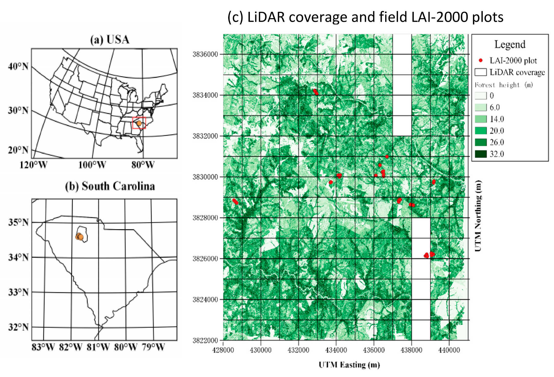
2.1. Study Area
2.2. Datasets and Preprocessing
2.2.1. Field Measured Data
2.2.2. LiDAR Data
2.2.3. Airborne Hyperspectral Data
2.3. Methodology
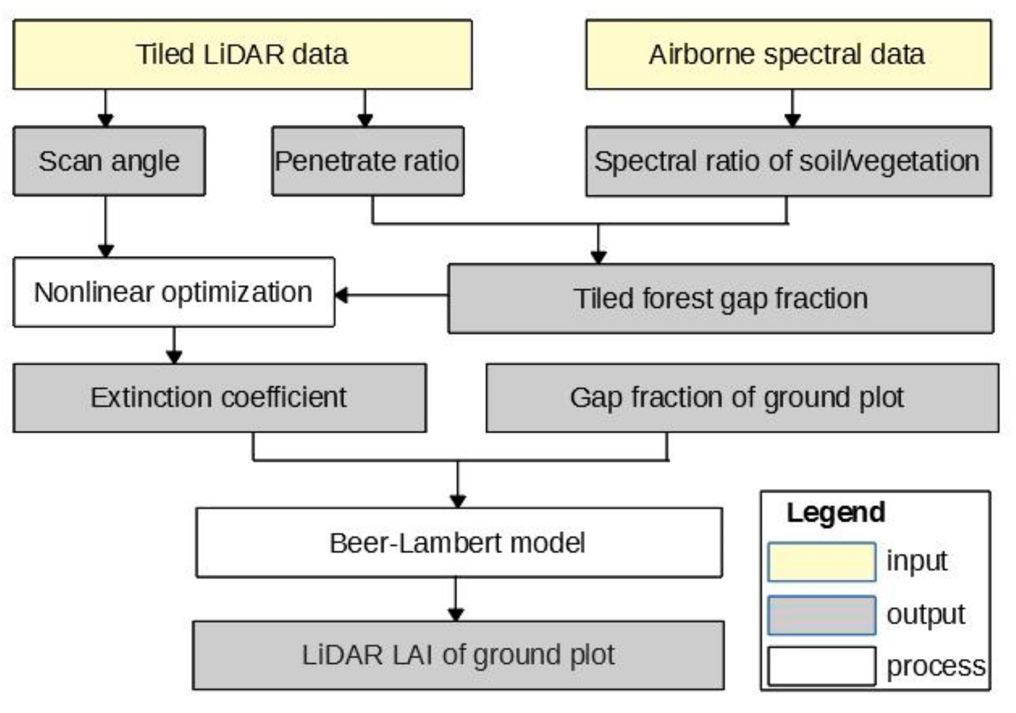
2.3.1. Overview
2.3.2. Spectral Correction Coefficient
2.3.3. Gap Fraction from Spectrally Corrected LiDAR Penetration Ratio
2.3.4. LiDAR Extinction Coefficient
2.3.5. Plot Level LiDAR LAI
2.4. Evaluation
3. Results
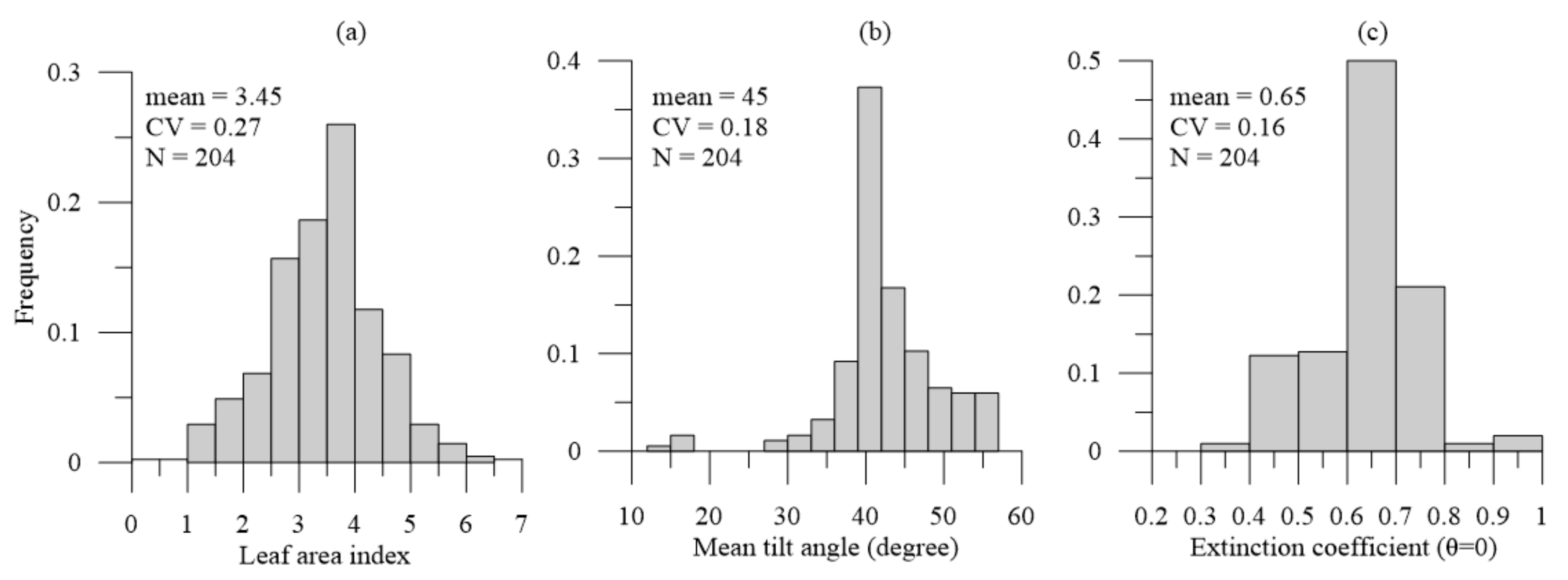
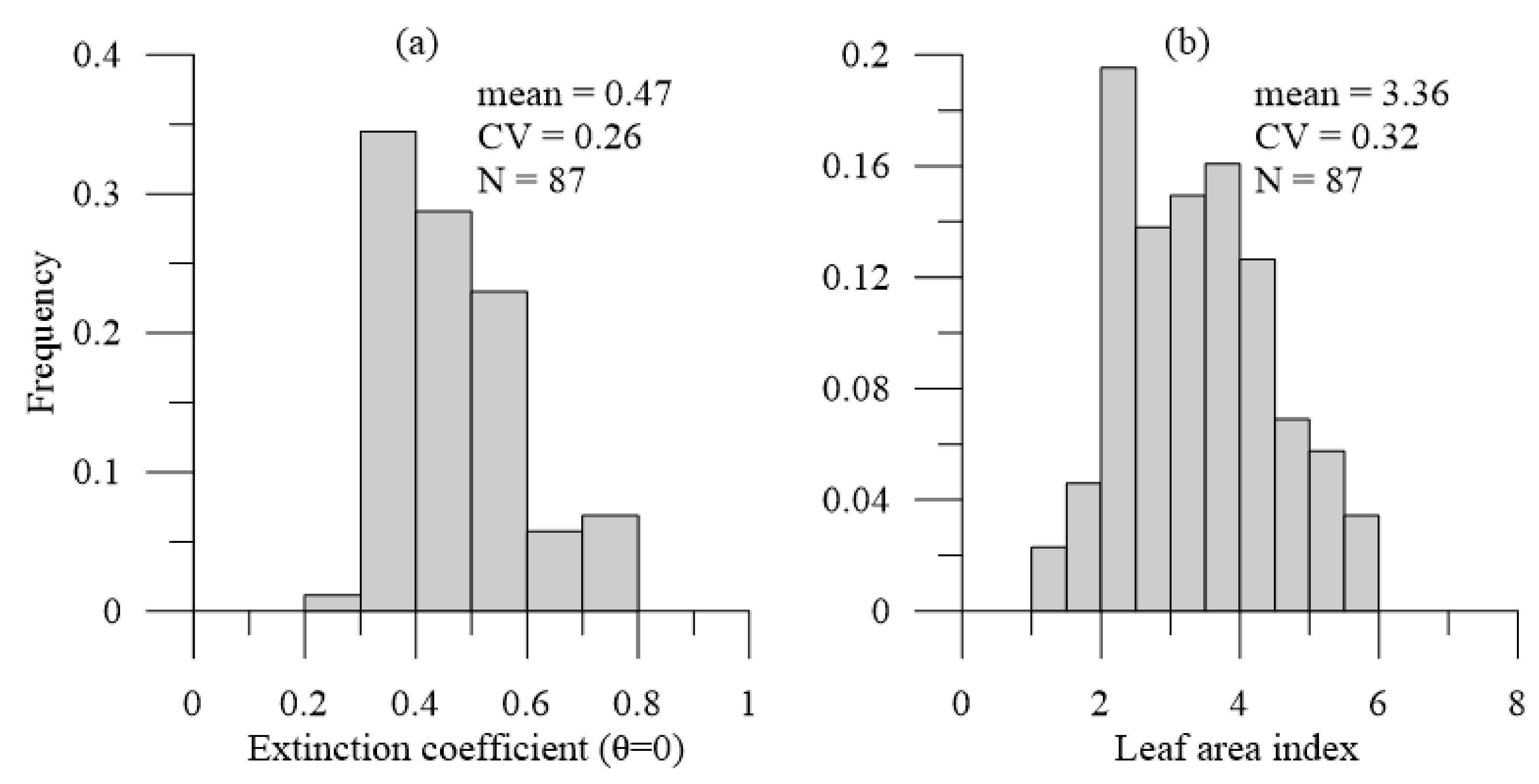
3.1. Statistical Features of Field Measurement
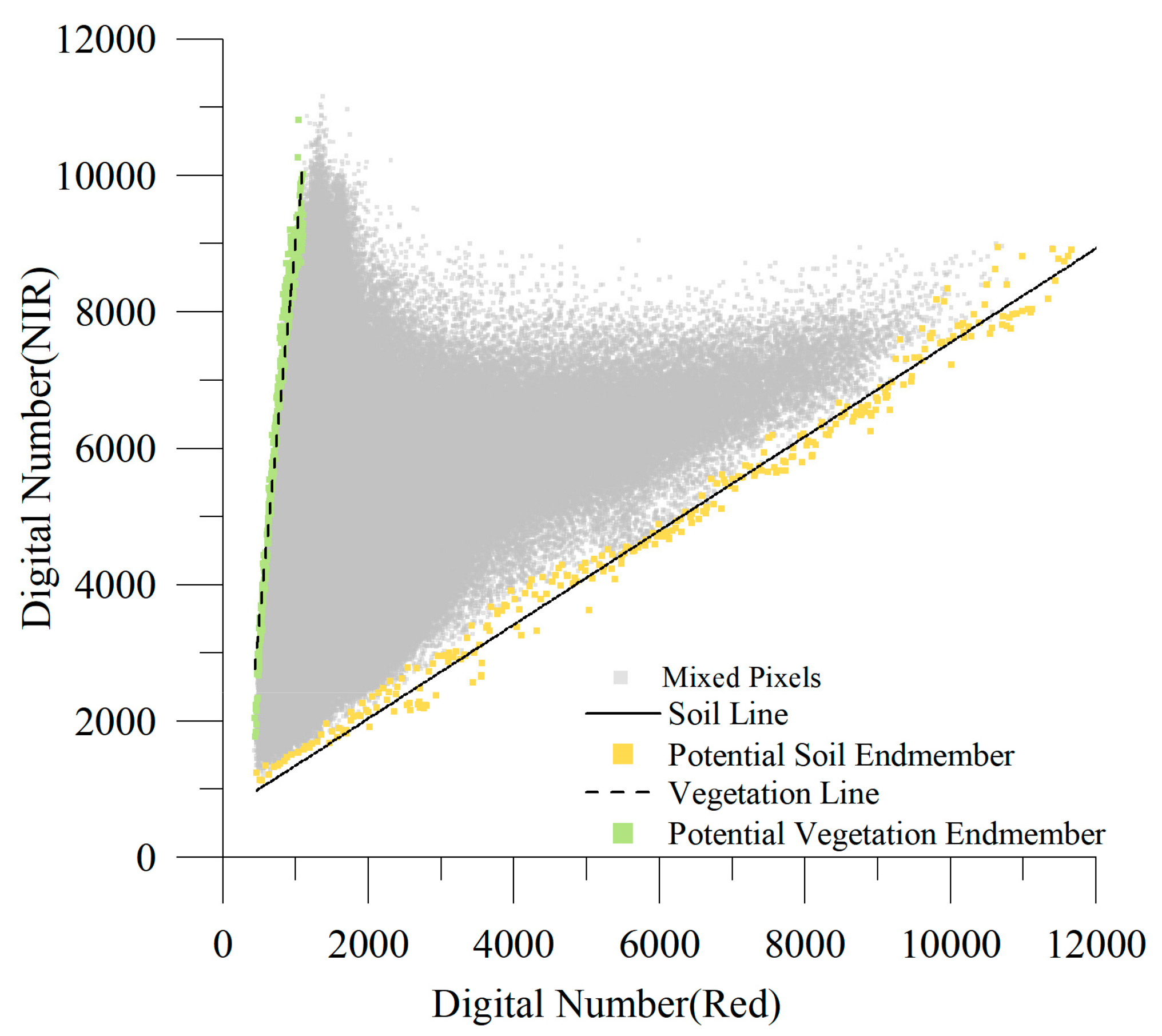
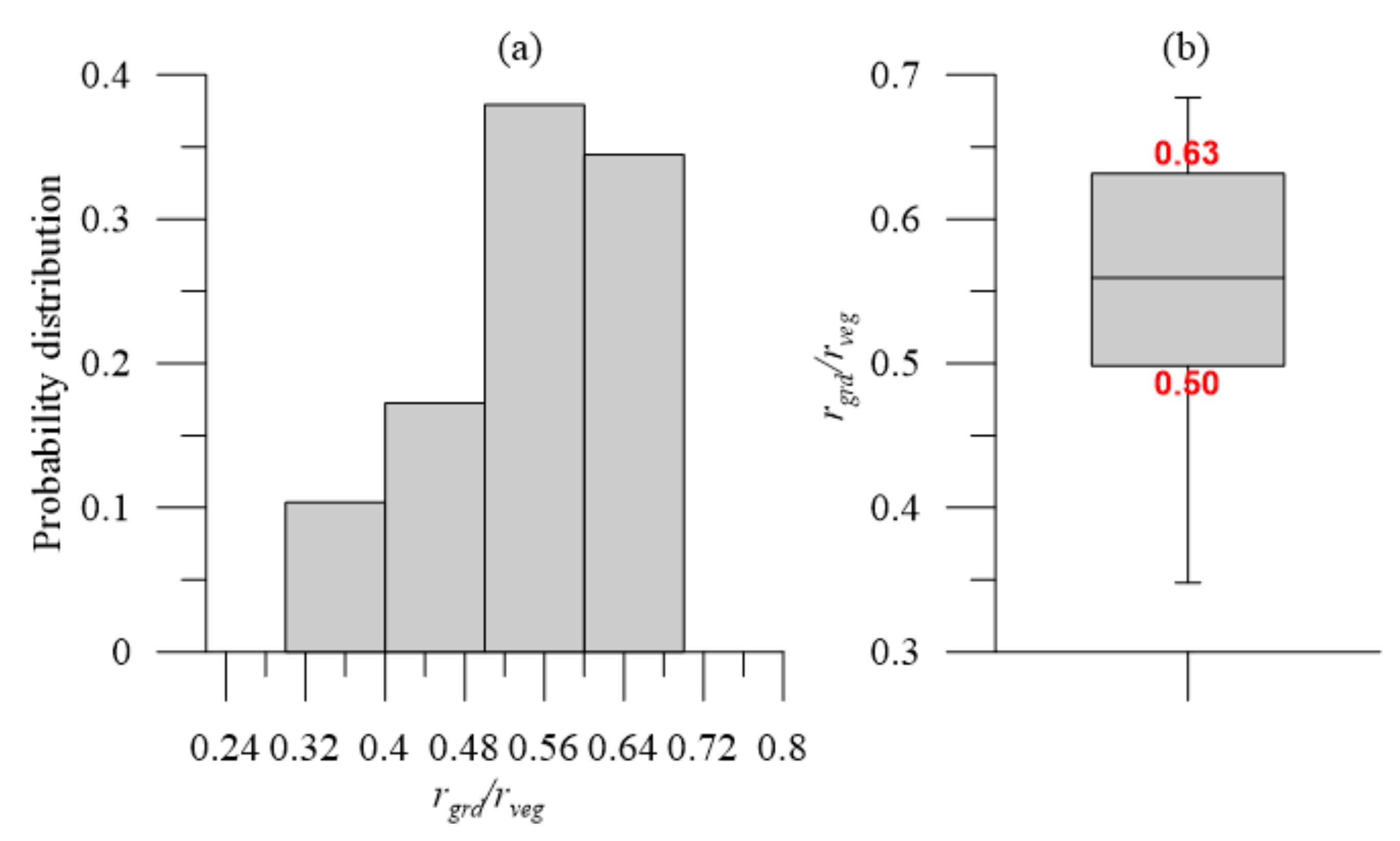
3.2. Spectral Ratio of Soil and Vegetation
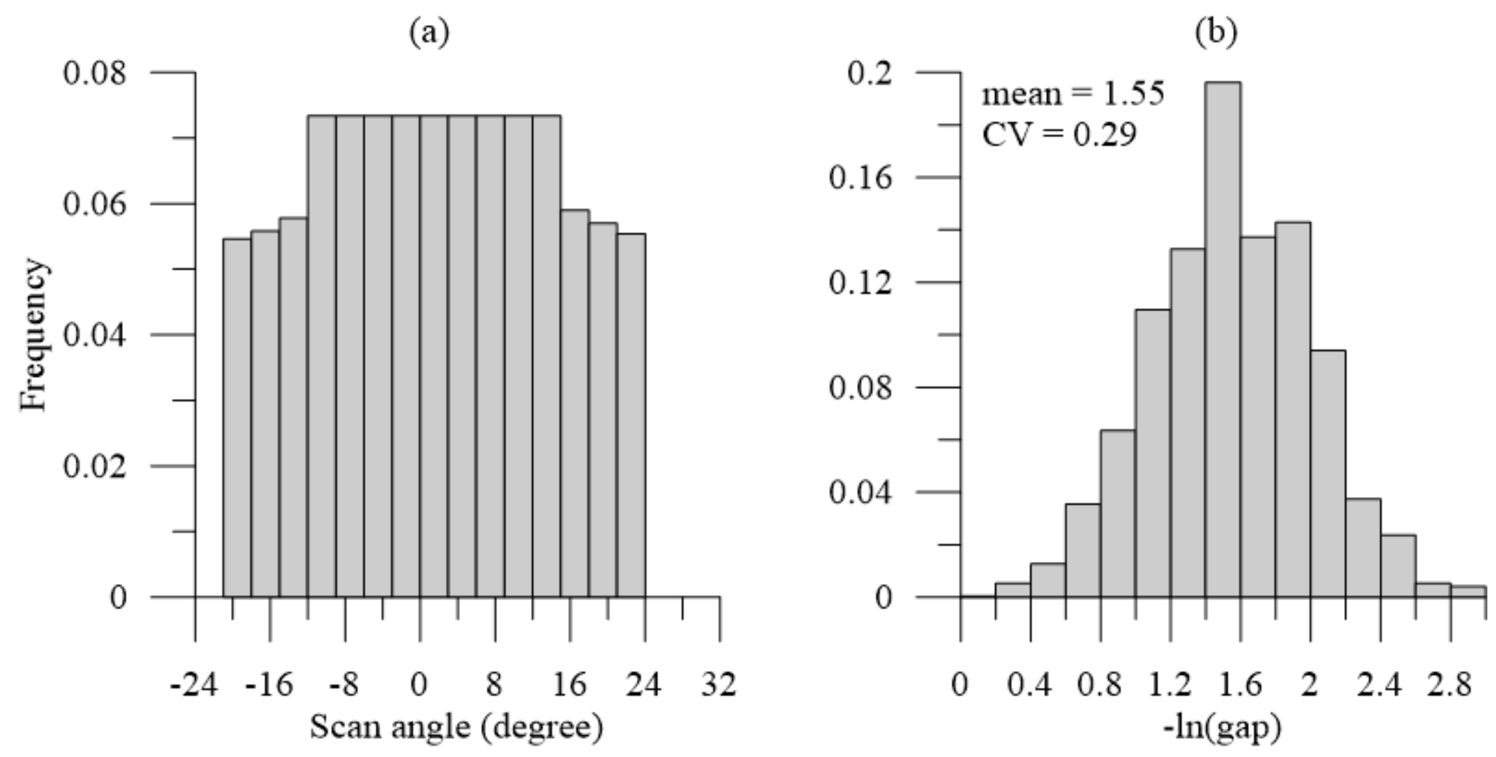
3.3. LiDAR Gap Fraction
3.4. Tile-Level LiDAR Extinction Coefficient and LAI
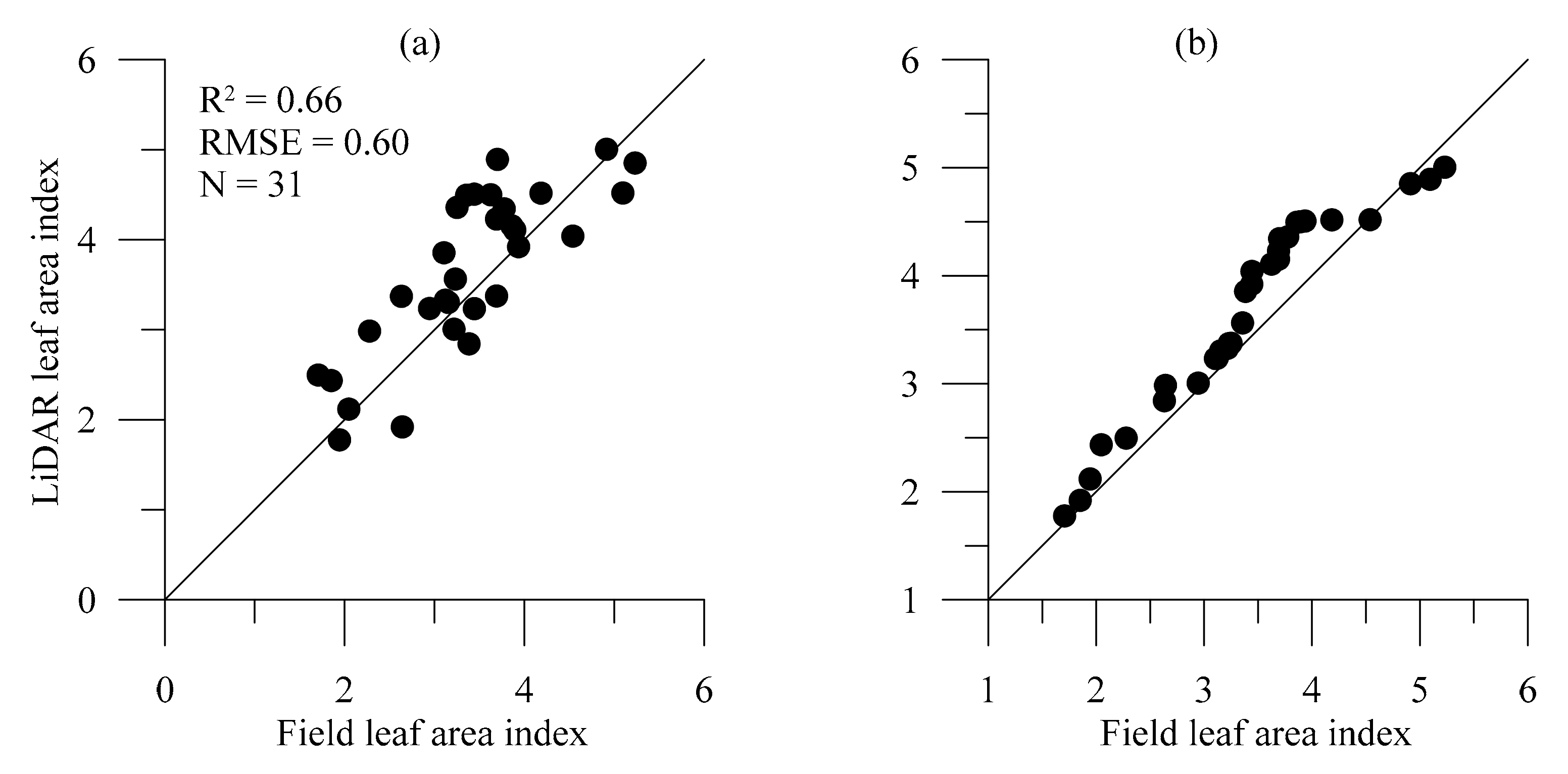
3.5. Plot-Level LiDAR LAI and Gap Fraction
4. Discussion
4.1. Performance of LiDAR LAI Estimation
4.2. Impact of Target Optical Property on LiDAR-Derived LAI
4.3. On the Constraints on Nonlinear Optimization
5. Conclusions
- (1)
- It is feasible to retrieve forest LAI from discrete LiDAR data without field data when the forest gap fraction and extinction coefficient can be appropriately calculated.
- (2)
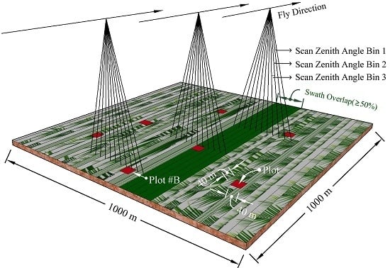
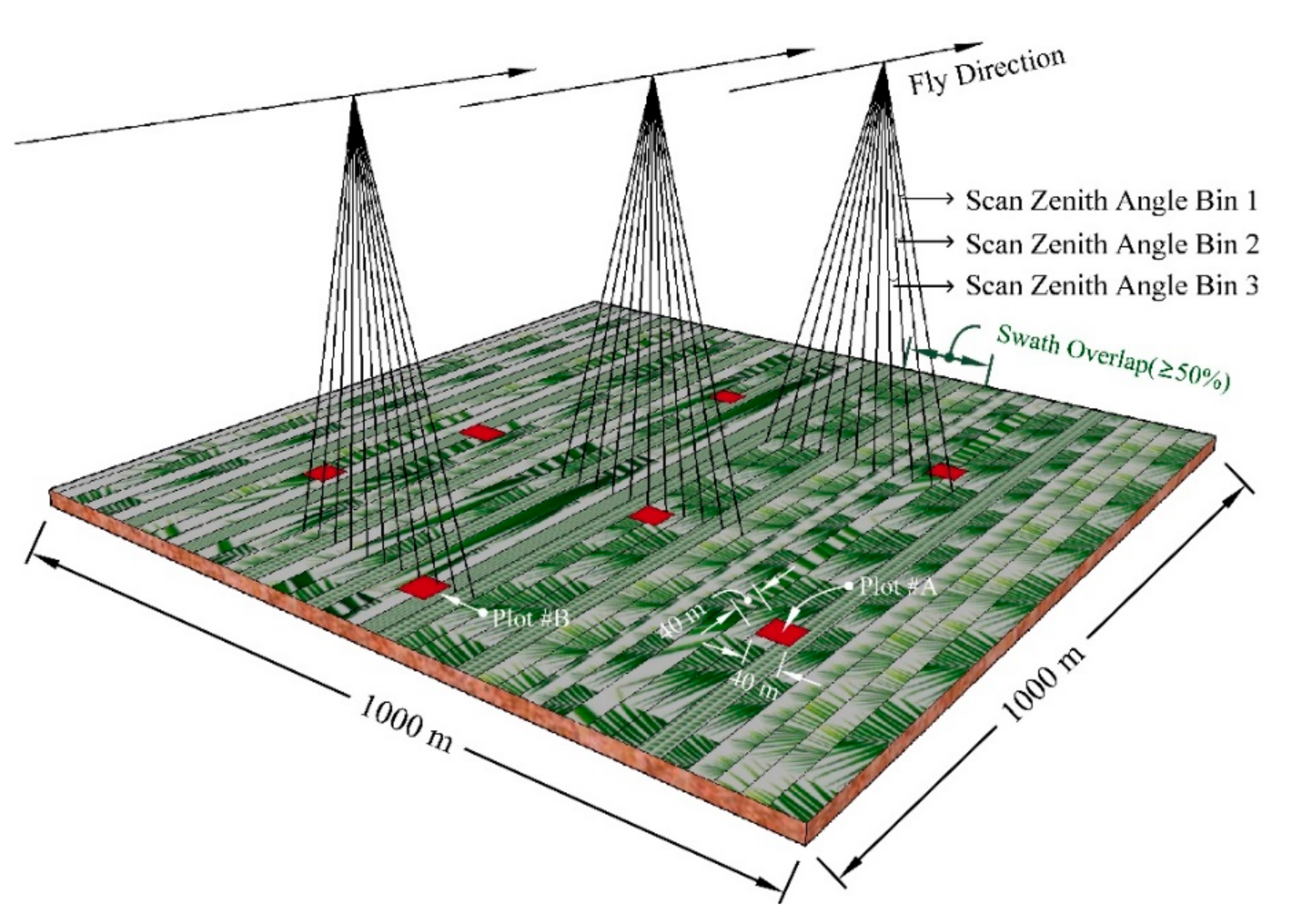
- Angular gap fractions can be obtained from large tiles of LiDAR data, which usually have a much larger range of scan zenith angles than plot-level data.
- (3)
- For tiled data, the inversion of the Beer–Lambert law-based model provides a feasible method to retrieve tile-level LAI and extinction coefficients.
- (4)
- Statistics for the tile-level extinction coefficient are valid for the plot-level LiDAR to estimate LAI corresponding to field measurements.
Author Contributions
Funding
Acknowledgments
Conflicts of Interest
References
- Chen, J.M.; Black, T.A. Defining leaf area index for non-flat leaves. Plant Cell Environ. 1992, 15, 421–429. [Google Scholar] [CrossRef]
- Myneni, R.B.; Yang, W.; Nemani, R.R.; Huete, A.R.; Dickinson, R.E.; Knyazikhin, Y.; Didan, K.; Fu, R.; Negron Juarez, R.I.; Saatchi, S.S.; et al. Large seasonal swings in leaf area of Amazon rainforests. Proc. Natl. Acad. Sci. USA 2007, 104, 4820–4823. [Google Scholar] [CrossRef] [PubMed]
- Myneni, R.B.; Hoffman, S.; Knyazikhin, Y.; Privette, J.L.; Glassy, J.; Tian, Y.; Wang, Y.; Song, X.; Zhang, Y.; Smith, G.R. Global products of vegetation leaf area and fraction absorbed PAR from year one of MODIS data. Remote Sens. Environ. 2002, 83, 214–231. [Google Scholar] [CrossRef]
- Tang, H.; Dubayah, R.; Swatantran, A.; Hofton, M.; Sheldon, S.; Clark, D.B.; Blair, B. Retrieval of vertical LAI profiles over tropical rain forests using waveform lidar at La Selva, Costa Rica. Remote Sens. Environ. 2012, 124, 242–250. [Google Scholar] [CrossRef]
- Lefsky, M.A.; Cohen, W.B.; Acker, S.A.; Parker, G.G.; Spies, T.A.; Harding, D. Lidar Remote Sensing of the Canopy Structure and Biophysical Properties of Douglas-Fir Western Hemlock Forests. Remote Sens. Environ. 1999, 70, 339–361. [Google Scholar] [CrossRef]
- Riaño, D.; Valladares, F.; Condés, S.; Chuvieco, E. Estimation of leaf area index and covered ground from airborne laser scanner (Lidar) in two contrasting forests. Agric. For. Meteorol. 2004, 124, 269–275. [Google Scholar] [CrossRef]
- Farid, A.; Goodrich, D.C.; Bryant, R.; Sorooshian, S. Using airborne lidar to predict Leaf Area Index in cottonwood trees and refine riparian water-use estimates. J. Arid Environ. 2008, 72, 1–15. [Google Scholar] [CrossRef]
- Qu, Y.; Shaker, A.; Silva, C.; Klauberg, C.; Pinagé, E. Remote Sensing of Leaf Area Index from LiDAR Height Percentile Metrics and Comparison with MODIS Product in a Selectively Logged Tropical Forest Area in Eastern Amazonia. Remote Sens. 2018, 10, 970. [Google Scholar] [CrossRef]
- Alonzo, M.; Bookhagen, B.; McFadden, J.P.; Sun, A.; Roberts, D.A. Mapping urban forest leaf area index with airborne lidar using penetration metrics and allometry. Remote Sens. Environ. 2015, 162, 141–153. [Google Scholar] [CrossRef]
- Sasaki, T.; Imanishi, J.; Ioki, K.; Song, Y.; Morimoto, Y. Estimation of leaf area index and gap fraction in two broad-leaved forests by using small-footprint airborne LiDAR. Landsc. Ecol. Eng. 2016, 12, 117–127. [Google Scholar] [CrossRef]
- Hopkinson, C.; Chasmer, L.E. Modelling canopy gap fraction from lidar intensity. In Proceedings of the ISPRS Workshop on Laser Scanning 2007 and SilviLaser 2007, Espoo, Finland, 12–14 September 2007; ISPRS: Espoo, Finland, 2007; pp. 190–194. [Google Scholar]
- Nilson, T. A theoretical analysis of the frequency of gaps in plant stands. Agric. Meteorol. 1971, 8, 25–38. [Google Scholar] [CrossRef]
- Frank, T.D.; Tweddale, S.A.; Lenschow, S.J. Non-destructive estimation of canopy gap fractions and shrub canopy volume of dominant shrub species in the Mojave desert. J. Terramech. 2005, 42, 231–244. [Google Scholar] [CrossRef]
- Solberg, S. Mapping gap fraction, LAI and defoliation using various ALS penetration variables. Int. J. Remote Sens. 2010, 31, 1227–1244. [Google Scholar] [CrossRef]
- Korhonen, L.; Korpela, I.; Heiskanen, J.; Maltamo, M. Airborne discrete-return LIDAR data in the estimation of vertical canopy cover, angular canopy closure and leaf area index. Remote Sens. Environ. 2011, 115, 1065–1080. [Google Scholar] [CrossRef]
- Heiskanen, J.; Korhonen, L.; Hietanen, J.; Pellikka, P.K.E. Use of airborne lidar for estimating canopy gap fraction and leaf area index of tropical montane forests. Int. J. Remote Sens. 2015, 36, 2569–2583. [Google Scholar] [CrossRef]
- Armston, J.; Disney, M.; Lewis, P.; Scarth, P.; Phinn, S.; Lucas, R.; Bunting, P.; Goodwin, N. Direct retrieval of canopy gap probability using airborne waveform lidar. Remote Sens. Environ. 2013, 134, 24–38. [Google Scholar] [CrossRef]
- Ni-Meister, W.; Jupp, D.L.B.; Dubayah, R. Modeling lidar waveforms in heterogeneous and discrete canopies. IEEE Trans. Geosci. Remote Sens. 2001, 39, 1943–1958. [Google Scholar] [CrossRef]
- Chen, X.T.; Disney, M.I.; Lewis, P.; Armston, J.; Han, J.T.; Li, J.C. Sensitivity of direct canopy gap fraction retrieval from airborne waveform lidar to topography and survey characteristics. Remote Sens. Environ. 2014, 143, 15–25. [Google Scholar] [CrossRef]
- Wang, W.M.; Li, Z.L.; Su, H.B. Comparison of leaf angle distribution functions: Effects on extinction coefficient and fraction of sunlit foliage. Agric. For. Meteorol. 2007, 143, 106–122. [Google Scholar] [CrossRef]
- Campbell, G.S. Extinction coefficients for radiation in plant canopies calculated using an ellipsoidal inclination angle distribution. Agric. For. Meteorol. 1986, 317–321. [Google Scholar] [CrossRef]
- Martens, S.N.; Ustin, S.L.; Rousseau, R.A. Estimation of tree canopy leaf area index by gap fraction analysis. For. Ecol. Manag. 1993, 61, 91–108. [Google Scholar] [CrossRef]
- Pisek, J.; Sonnentag, O.; Richardson, A.D.; Mõttus, M. Is the spherical leaf inclination angle distribution a valid assumption for temperate and boreal broadleaf tree species? Agric. For. Meteorol. 2013, 169, 186–194. [Google Scholar] [CrossRef]
- Korhonen, L.; Morsdorf, F. Estimation of canopy cover, gap fraction and leaf area index with airborne laser scanning. In Forestry Applications of Airborne Laser Scanning- Concepts and Case Studies. Managing Forest Ecosystems 27; Maltamo, M., Næsset, E., Vauhkonen, J., Eds.; Springer Science + Business Media: Dordrecht, The Netherlands, 2014; p. 464. [Google Scholar]
- Zheng, G.; Ma, L.; Eitel, J.U.H.; He, W.; Magney, T.S.; Moskal, L.M.; Li, M. Retrieving Directional Gap Fraction, Extinction Coefficient, and Effective Leaf Area Index by Incorporating Scan Angle Information From Discrete Aerial Lidar Data. IEEE Trans. Geosci. Remote Sens. 2017, 55, 577–590. [Google Scholar] [CrossRef]
- Coughlan, M.R.; Nelson, D.R.; Lonneman, M.; Block, A.E. Historical Land Use Dynamics in the Highly Degraded Landscape of the Calhoun Critical Zone Observatory. Land 2017, 6, 32. [Google Scholar] [CrossRef]
- Cook, C.W.; Brecheisen, Z.; Richter, D.D. CZO Dataset: Calhoun CZO—Vegetation (2014–2017)—Tree Survey. Available online: http://criticalzone.org/calhoun/data/dataset/4614/ (accessed on 6 January 2020).
- Campbell, G.S. Derivation of an angle density function for canopies with ellipsoidal leaf angle distributions. Agric. For. Meteorol. 1990, 49, 173–176. [Google Scholar] [CrossRef]
- Chen, J.M.; Plummer, P.S.; Rich, M.; Gower, S.T.; Norman, J.M. Leaf area index of boreal forests: Theory, techniques, and measurements. J. Geophys. Res. 1997, 102, 29429–29443. [Google Scholar] [CrossRef]
- Parkan, M. Digital Forestry Toolbox for Matlab/Octave. 2018. Available online: http://mparkan.github.io/Digital-Forestry-Toolbox (accessed on 6 January 2020). [CrossRef]
- Fox, G.A.; Sabbagh, G.J.; Searcy, S.W.; Yang, C. An Automated Soil Line Identification Routine for Remotely Sensed Images. Soil Sci. Soc. Am. J. 2004, 68, 1326–1331. [Google Scholar] [CrossRef]
- Gitelson, A.A.; Stark, R.; Grits, U.; Rundquist, D.; Kaufman, Y.; Derry, D. Vegetation and soil lines in visible spectral space: A concept and technique for remote estimation of vegetation fraction. Int. J. Remote Sens. 2002, 23, 2537–2562. [Google Scholar] [CrossRef]
- Jia, K.; Li, Y.; Liang, S.; Wei, X.; Mu, X.; Yao, Y. Fractional vegetation cover estimation based on soil and vegetation lines in a corn-dominated area. Geocarto Int. 2017, 32, 531–540. [Google Scholar] [CrossRef]
- Bojinski, S.; Schaepman, M.; Schläpfer, D.; Itten, K. SPECCHIO: A spectrum database for remote sensing applications. Comput. Geosci.-Uk 2003, 29, 27–38. [Google Scholar] [CrossRef]
- Solberg, S.; Næsset, E.; Hanssen, K.H.; Christiansen, E. Mapping defoliation during a severe insect attack on Scots pine using airborne laser scanning. Remote Sens. Environ. 2006, 102, 364–376. [Google Scholar] [CrossRef]
- Hovi, A. Towards an enhanced understanding of airborne LiDAR measurements of forest vegetation. University of Helsinki. Diss. For. 2015. [Google Scholar] [CrossRef]
- Ni-Meister, W.; Yang, W.; Lee, S.; Strahler, A.H.; Zhao, F. Validating modeled lidar waveforms in forest canopies with airborne laser scanning data. Remote Sens. Environ. 2018, 204, 229–243. [Google Scholar] [CrossRef]
- Fleck, S.; Raspe, S.; Cater, M.; Schleppi, P.; Ukonmaanaho, L.; Greve, M.; Hertel, C.; Weis, W.; Rumpf, S.; Thimonier, A.; et al. Part XVII: Leaf Area Measurements. Available online: http://www.icp-forests.org/pdf/manual/2016/ICP_Manual_2016_01_part17.pdf (accessed on 6 January 2020).
- Hu, R.; Yan, G.; Nerry, F.; Liu, Y.; Jiang, Y.; Wang, S.; Chen, Y.; Mu, X.; Zhang, W.; Xie, D. Using Airborne Laser Scanner and Path Length Distribution Model to Quantify Clumping Effect and Estimate Leaf Area Index. IEEE Trans. Geosci. Remote Sens. 2018, 56, 3196–3209. [Google Scholar] [CrossRef]
- Scurlock, J.M.O.; Asner, G.P.; Gower, S.T. Global Leaf Area Index Data from Field Measurements, 1932–2000; Oak Ridge National Laboratory Distributed Active Archive Center: Oak Ridge, TN, USA, 2001. Available online: https://daac.ornl.gov/ (accessed on 6 January 2020).
- Majasalmi, T.; Palmroth, S.; Cook, W.; Brecheisen, Z.; Richter, D. Estimation of LAI, fPAR and AGB based on data from Landsat 8 and LiDAR at the Calhoun CZO. In Proceedings of the Calhoun CZO 2015 Summer Science Meeting, Union County, NC, USA, 29–30 June 2015; Calhoun Experimental Forest: Union County, NC, USA, 2015. [Google Scholar]
- Solberg, S.; Brunner, A.; Hanssen, K.H.; Lange, H.; Næsset, E.; Rautiainen, M.; Stenberg, P. Mapping LAI in a Norway spruce forest using airborne laser scanning. Remote Sens. Environ. 2009, 113, 2317–2327. [Google Scholar] [CrossRef]
- Ma, H.; Song, J.; Wang, J. Forest Canopy LAI and Vertical FAVD Profile Inversion from Airborne Full-Waveform LiDAR Data Based on a Radiative Transfer Model. Remote Sens. 2015, 7, 1897–1914. [Google Scholar] [CrossRef]
- Ma, H.; Song, J.; Wang, J.; Xiao, Z.; Fu, Z. Improvement of spatially continuous forest LAI retrieval by integration of discrete airborne LiDAR and remote sensing multi-angle optical data. Agric. For. Meteorol. 2014, 189, 60–70. [Google Scholar] [CrossRef]
- Ma, L.; Zheng, G.; Wang, X.; Li, S.; Lin, Y.; Ju, W. Retrieving forest canopy clumping index using terrestrial laser scanning data. Remote Sens. Environ. 2018, 210, 452–472. [Google Scholar] [CrossRef]
- Hopkinson, C.; Lovell, J.; Chasmer, L.; Jupp, D.; Kljun, N.; van Gorsel, E. Integrating terrestrial and airborne lidar to calibrate a 3D canopy model of effective leaf area index. Remote Sens. Environ. 2013, 136, 301–314. [Google Scholar] [CrossRef]
- Li, X.; Gao, F.; Wang, J.; Strahler, A. A priori knowledge accumulation and its application to linear BRDF model inversion. J. Geophys. Res. 2001, 106, 11925–11935. [Google Scholar] [CrossRef]
- Teske, M.E.; Thistle, H.W. A library of forest canopy structure for use in interception modeling. For. Ecol. Manag. 2004, 198, 341–350. [Google Scholar] [CrossRef]
- Rautiainen, M.; Stenberg, P. On the angular dependency of canopy gap fractions in pine, spruce and birch stands. Agric. For. Meteorol. 2015, 206, 1–3. [Google Scholar] [CrossRef]
- Embrapa. Web System Offers LiDAR Data on Brazilian Biomes. Available online: https://www.embrapa.br/en/busca-de-noticias/-/noticia/15706279/web-system-offers-lidar-data-on-brazilian-biomes (accessed on 12 July 2019).


| Nominal Flight Parameters | Equipment Settings | ||
|---|---|---|---|
| Flight altitude | 500 m | Laser PRF * | 100 kHz |
| Flight speed | ±65 m/s | Beam Divergence | 0.80 mrad |
| Swath width | 268 m | Scan frequency | 60 Hz |
| Swath overlap | ≥50% | Mean scan angle | ±16° |
| Point density | 10.7 p/m2 | Scan cutoff | 1.0° |
| Parameter | Mean | Min. | Max. | Std. | Median |
|---|---|---|---|---|---|
| Gap Fraction | 0.21 | 0.10 | 0.45 | 0.092 | 0.17 |
| Scan Zenith Angle | 7.92 | 4.34 | 10.29 | 1.43 | 8.22 |
| # | Forest Type a | Min. LAI | Max. LAI | R2 | RMSE | RRMSE | N b | Sensor Platform c | Citation |
|---|---|---|---|---|---|---|---|---|---|
| 1 | BLF | 0.10 | 9.60 | 0.5/0.63 d | 1.79/1.36 d | 0.45/0.34 | 546/185 d | Waveform ALS | Tang et al. [4] Figure 3 |
| 2 | CLF | 2.23 | 4.61 | 0.53 | 0.67 | 0.19 | 15 | Waveform ALS | Ma et al. [43] Figure 9 |
| 3 | CLF | 0.89 | 4.90 | 0.66–0.73 e | 0.72–2.20 e | 0.20–0.68 e | 24 | Waveform ALS | Ma et al. [44] Figure 11 |
| 4 | MLF | 1.17 | 6.48 | 0.72 | 1.16 | 0.44 | 18 | Discrete ALS | Zheng et al. [25] Figure 6 |
| 5 | CLF | 0.27 | 8.77 | 0.62 | 1.59 | 0.42 | 30 | Discrete TLS | Ma et al. [45] Figure 12 |
| 6 | BLF | 1.30 | 1.90 | 0.64 | 1.20 | 0.76 | 8 | Discrete TLS | Hopkinson et al. [46] Figure 3 |
| 7 | CLF | 1.71 | 5.23 | 0.66 | 0.60 | 0.15 | 31 | Discrete ALS | This study |
© 2020 by the authors. Licensee MDPI, Basel, Switzerland. This article is an open access article distributed under the terms and conditions of the Creative Commons Attribution (CC BY) license (http://creativecommons.org/licenses/by/4.0/).
Share and Cite
Qu, Y.; Shaker, A.; Korhonen, L.; Silva, C.A.; Jia, K.; Tian, L.; Song, J. Direct Estimation of Forest Leaf Area Index based on Spectrally Corrected Airborne LiDAR Pulse Penetration Ratio. Remote Sens. 2020, 12, 217. https://doi.org/10.3390/rs12020217
Qu Y, Shaker A, Korhonen L, Silva CA, Jia K, Tian L, Song J. Direct Estimation of Forest Leaf Area Index based on Spectrally Corrected Airborne LiDAR Pulse Penetration Ratio. Remote Sensing. 2020; 12(2):217. https://doi.org/10.3390/rs12020217
Chicago/Turabian StyleQu, Yonghua, Ahmed Shaker, Lauri Korhonen, Carlos Alberto Silva, Kun Jia, Luo Tian, and Jinling Song. 2020. "Direct Estimation of Forest Leaf Area Index based on Spectrally Corrected Airborne LiDAR Pulse Penetration Ratio" Remote Sensing 12, no. 2: 217. https://doi.org/10.3390/rs12020217
APA StyleQu, Y., Shaker, A., Korhonen, L., Silva, C. A., Jia, K., Tian, L., & Song, J. (2020). Direct Estimation of Forest Leaf Area Index based on Spectrally Corrected Airborne LiDAR Pulse Penetration Ratio. Remote Sensing, 12(2), 217. https://doi.org/10.3390/rs12020217