An End-To-End Bayesian Segmentation Network Based on a Generative Adversarial Network for Remote Sensing Images

Abstract

Due to the development of deep convolutional neural networks (CNNs), great progress has been made in semantic segmentation recently. In this paper, we present an end-to-end Bayesian segmentation network based on generative adversarial networks (GANs) for remote sensing images. First, fully convolutional networks (FCNs) and GANs are utilized to realize the derivation of the prior probability and the likelihood to the posterior probability in Bayesian theory. Second, the cross-entropy loss in the FCN serves as an a priori to guide the training of the GAN, so as to avoid the problem of mode collapse during the training process. Third, the generator of the GAN is used as a teachable spatial filter to construct the spatial relationship between each label. Some experiments were performed on two remote sensing datasets, and the results demonstrate that the training of the proposed method is more stable than other GAN based models. The average accuracy and mean intersection (MIoU) of the two datasets were 0.0465 and 0.0821, and 0.0772 and 0.1708 higher than FCN, respectively.

1. Introduction

1.1. Background

The goal of image semantic segmentation is to predict a category label for each pixel in the image, which plays an important role in scene recognition. Many scene recognition applications, such as virtual or augmented reality, human–computer intersections [1], and autonomous driving [2,3], urgently need accurate and effective segmentation mechanisms. Driven by the these requirements, image semantic segmentation has gained more and more attention from machine learning and computer vision researchers.

Before deep learning took over computer vision, traditional image semantic segmentation methods were usually edge-based [4] or region-based [5]. Convolutional neural networks (CNNs) have achieved huge success in image segmentation [6,7,8] and with image classification. Patch image classification [9] was one of the initial deep learning methods to acquire popularity, in which each pixel was separately placed into a category using the surrounding image patches. However, the classification networks were usually designed as full connected layers, so fixed-size input images were required. In 2014, Long et al. proposed fully convolutional network (FCN) [10] which popularized the architectures of CNN for semantic segmentation without fully connected layers. This paradigm was adopted by almost all subsequent state of the art segmentation approaches. Many classic networks, such as AlexNet [11], VGG-16 [12], GoogLeNet [13], and ResNet [14] have been used as basic modules for many semantic segmentation architectures.

Currently, image semantic segmentation models based on deep learning can be roughly divided into three categories. The first one is the encoder-decoder neural network category, which includes U-Net [15] and SegNet [16]. In the encoder network, the spatial dimension is gradually reduced with a pooling layer. While in the decoder network, the spatial dimension and the object details are gradually recovered with up-sampling layers. The second one is called the dilated/atrous convolution neural network category, and includes Deeplab [17]. The atrous spatial pyramid pooling (ASPP) model and the fully connected conditional random field (CRF) are used in Deeplab, which can make better use of spatial information than FCN. The third one contains image pyramid neural networks, such as PSPNet [18]. Different pooling proportions are used to obtain features with different scales.

In addition to the semantic segmentation methods described above, a series of Bayesian framework-based methods [19,20,21,22,23,24,25] have been proposed. The Bayesian model is a statistical probability method, where the posterior probability is derived by calculating the prior probability and the likelihood function. Bayesian networks have been widely used in a range of applications. In the field of semantic segmentation, building a suitable Bayesian framework to make full use of prior probabilities and likelihood functions is the key. Pelizzari et al. [20] applied Bayesian segmentation to Oceanic SAR Images. They used loopy belief propagation (LBP) to estimate the smoothness parameter in the Markov random field (MRF) used as a prior in the framework, and applied graph-cut techniques to solve the energy minimization problem that arises from the followed Bayesian methodology. Zhang et al. [21] built the Bayesian network based on an edge map which integrates the a priori information such as regions, edges, and vertex nodes. Vezhnevets et al. [22] cast the problem of weakly supervised semantic segmentation as a Bayesian optimization problem and presented an algorithm based on Guassian processes to efficiently solve it. Ge et al. [23] proposed a semantic segmentation method based on neural network and Bayesian network, which employed Potts model [26] to model the prior distribution of labels, and utilized the Bayesian network to perform images of classification. In the literature [24], a deep learning based architecture for probabilistic pixel-wise segmentation was presented, which was achieved by Monte Carlo sampling with dropout during testing to produce a posterior distribution of class labels for each pixel. In the literature [25], Coombes et al. aimed to utilize a Bayesian network to implement probabilistic data fusion to classify a pre-segmented image.

In recent years, the generative adversarial network (GAN) [27], being an excellent framework, has attracted widespread attention from researchers. GAN inspired by a two-player, zero-sum game, consists of a discriminator and a generator. GAN improves its performance through adversarial training, which can be described as the generator trying to obtain the latent distribution of real data and producing fake data to cheat the discriminator, while the discriminator tries to distinguish real data from fake data as much as possible. The generator and discriminator compete with each other in training process. This adversarial model has been widely used in different applications. Luc et al. [28] first used GAN to image segmentation for the purpose of enhancing long-range spatial label contiguity without increasing the complexity of the model used in the test. Subsequently, a variety of GAN-based segmentation methods [29,30,31,32,33,34,35] were proposed. Zhu et al. [29] proposed an end-to-end network with the trained adversarial deep structure to improve the robustness of a small data model and prevent over-fitting. This algorithm utilizes FCN to classify images at the pixel level, and CRF to implement structural learning to capture high-order potentials. In the paper [30] that the pix2pix software is associated with, Phillip et al. applied conditional GAN to image-to-image translation problems, including image segmentation tasks. PatchGAN was first applied to discriminant networks. Huo et al. [33] applied GAN to splenomegaly segmentation, in which the global convolutional network (GCN) was employed as the generator designed to alleviate false negatives and the PatchGAN [33] was applied to reduce false positives. For remote sensing images, Ma et al. [34] proposed a weakly supervised approach, which integrates CRF and hierarchical conditional generative adversarial (cGAN) nets to conduct the segmentation for high-resolution SAR images. Although a large quantity of approaches have been presented in the literature, the problem of semantic segmentation has not been completely solved.

1.2. Problems and Motivations

FCN was groundbreaking in the area of semantic segmentation, and has received considerable attention. However, the labels predicted by FCN lack of a basic spatial relationship or contextual information, resulting in a coarser segmentation result. In Bayesian theory, this method can be said to have no complete derivation from the prior probability and the likelihood function to the posterior probability. The FCN only uses the current pixel and neighborhood pixels to predict each label, completely ignoring the relationships between the labels. In other words, the FCN only makes proper use of the prior probability between pixels and ignores the likelihood knowledge of the label.

On the basis of FCN, Deeplab uses the fully connected CRF as an independent post-processing stage to build the spatial relationship between labels. The performance of segmentation is improved by exploiting the spatial relationship or context by using the one-potential and pairwise potentials in the CRF. However, this apparent spatial relationship is prone to local optimal problems. In essence, it is difficult for Deeplab to achieve global optimization in the Bayesian framework.

Pix2pix constructs the potential spatial relationship between labels through conditional GAN. Although this potential spatial relationship is not as formulable as CRF, it may be more globally optimal when using the training of the GAN. However, pix2pix does not make full use of prior knowledge, and GAN can easily lead to mode collapse in the absence of guidance. It is well known that the adversarial training in GAN requires competition between the generator and the discriminator to improve network performance. This unguided competition may cause the training to be very unstable. For example, when the competence of discriminators is far more than that of generators, GAN may converge to a local extreme during training, which can lead to mode collapse. This problem still exists in GAN-based segmentation methods, although most papers do not point it out.

It can be seen that neither FCN nor Deeplab nor pix2pix have built a reasonable Bayesian framework for image segmentation. To fix this problem, it is necessary to construct a segmentation network under the Bayesian framework from both the prior network and the likelihood network. Therefore, this paper attempts to make full use of the advantages of FCN and GAN to construct a well-structured Bayesian network for remote sensing images’ segmentation.

1.3. Contribution and Structure

In this paper, we present an end-to-end Bayesian segmentation network based on a generative adversarial network to apply semantic segmentation to remote sensing images. Some key contributions of our work are as follows:

(1)

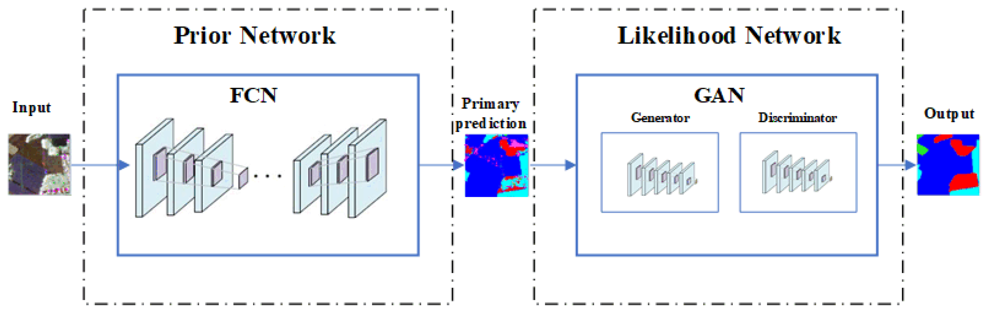
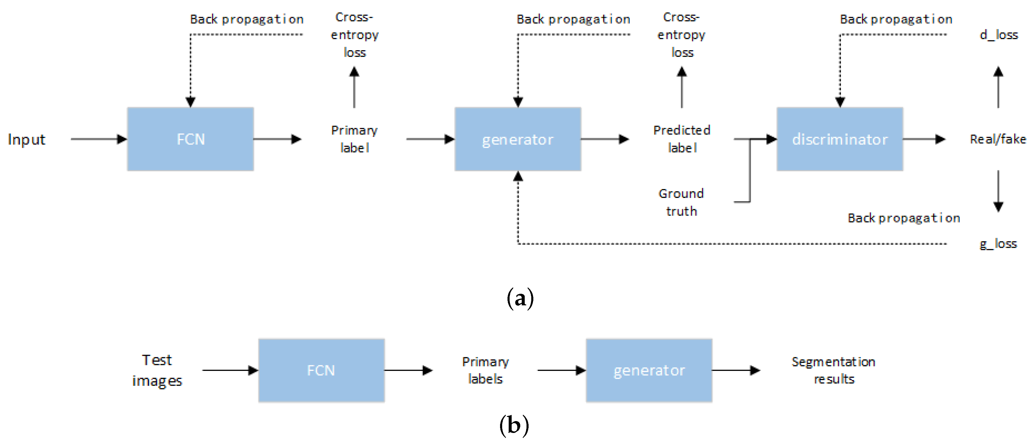
An end-to-end Bayesian segmentation network was designed, which uses FCN and GAN to achieve the derivation of the prior probability and likelihood function to the posterior probability. In the entire network architecture, FCN is used as the prior network, while GAN can be used as the likelihood network. The cross-entropy loss in the FCN is directly associated with the prior probability, and the loss of the GAN is correlated with the likelihood probability. Thus, a complete Bayesian framework has been constructed.

(2)

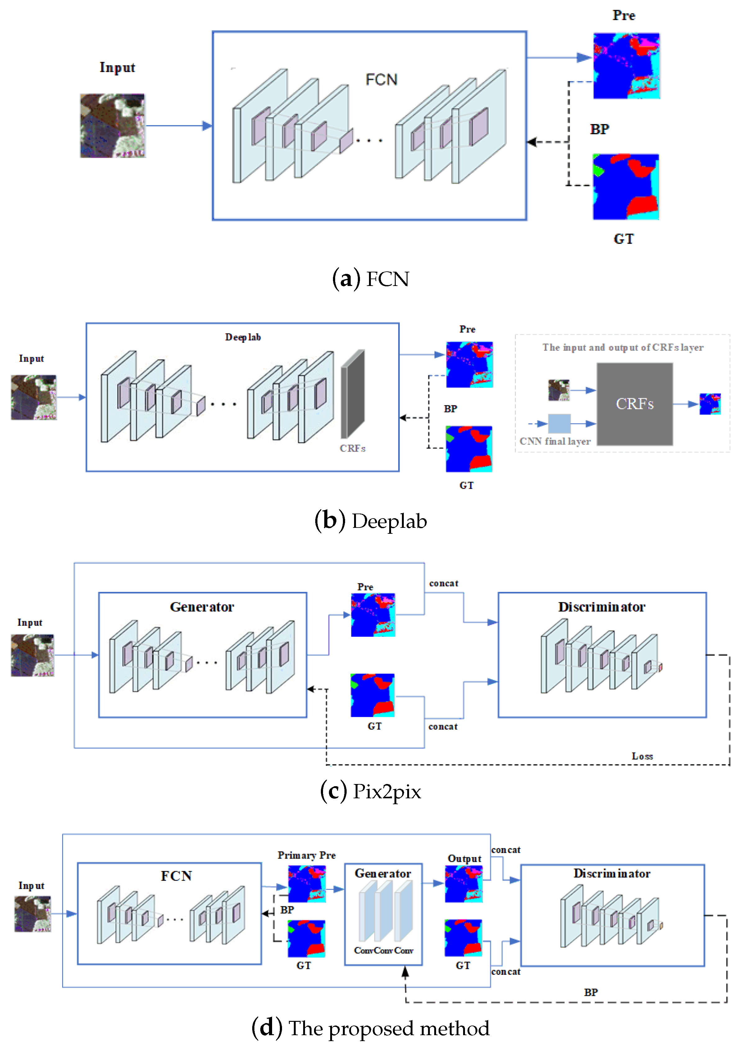
The cross-entropy loss in the FCN and the loss in the GAN are separately trained, rather than just using cross-entropy loss as part of the loss of a GAN generator. In the absence of effective guidance, GAN may often be plagued by the problem of model crashes. Therefore, we use the cross-entropy loss of FCN as an a priori guide for the training of GAN to make the network converge to global optimality. We verified that the proposed approach can not only improve the segmentation performance, but also enhance the stability of training.

(3)

The generator of GAN acts as a spatial filter which is integrated into the semantic segmentation framework to explore the spatial relationship between each label and optimize the results of the prior network. Unlike other GAN-based segmentation methods, the input of the generator is the output of the FCN instead of the image that needs to be predicted. It can be seen that the function of GAN is to further optimize the results obtained by FCN. Therefore, we provide a viable architecture for semantic segmentation.

The remainder of the manuscript has been structured as follows. In Section 2, the methodology is described in detail. In Section 3, we present the training and testing process of the network and set the relevant parameters. Section 4 provides experimental results and corresponding analysis. In Section 5 we discuss of the proposed method. Finally, Section 6 makes concluding remarks on our proposed work.

2. Methodology

2.1. Bayesian Segmentation Network

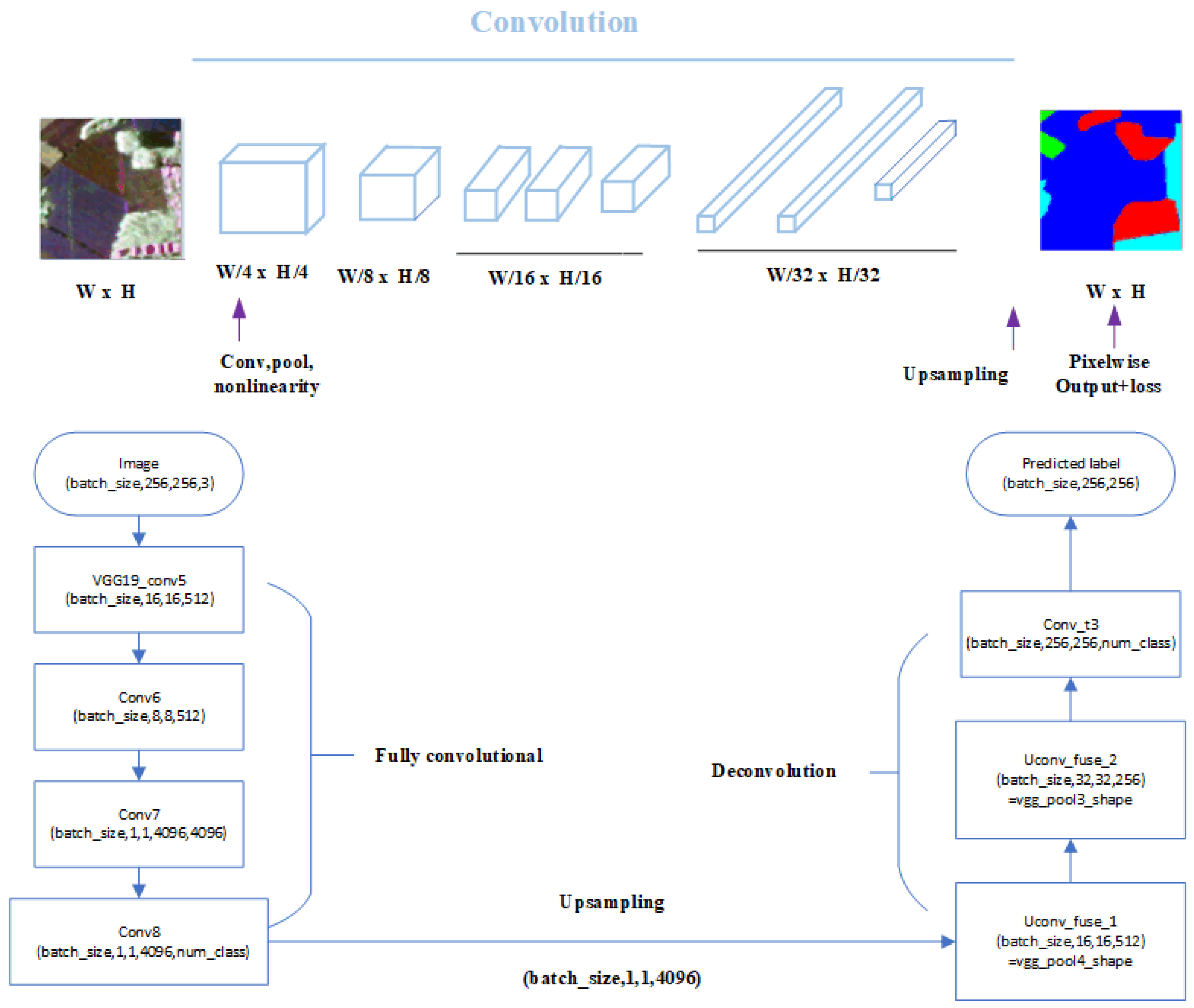
A Bayesian network is an important application of Bayesian inference which produces the posterior probability from the result of two elements: a “likelihood function” and a prior probability derived from a statistical model for the observed data. Bayesian inference calculates the posterior probability based on Bayes’ theorem:

$$P\left(A\right|B)=\frac{P\left(B\right|A\left)P\right(A)}{P\left(B\right)},$$

(1)

where A represents any hypothesis that its probability may be affected by data, and B represents the evidence, which corresponds to new data. P(A) is the prior probability, which stands for the estimate of the probability of the hypothesis A before the data B. P(B) is the current evidence, which is observed. P(A|B), the posterior probability, is the probability of A given B; i.e., after B is observed. P(B|A) is the probability of observing B given A, and is called the likelihood. P(B) is sometimes termed the model evidence which does not enter into determining the relative probabilities of different hypotheses. So the following formula can be derived:

$$P\left(A\right|B)\propto P(A)\ast P(B\left|A\right),$$

(2)

where the symbol ∝ stands for directly proportional. In other words, the posterior probability is proportional to its prior probability and the likelihood.

In the image segmentation task, in order to use the contextual information reasonably, constructing a prior network and a likelihood network are the keys. Figure 1 shows the basic framework of the proposed Bayesian segmentation network. It can been seen that the proposed network consists of two sub-network modules: a prior network and a likelihood network. FCN, the prior network, gets a preliminary segmentation result, and GAN, the likelihood network, explores the potential spatial relationship between labels to optimize the output of the FCN. In Figure 2, we present the segmentation frameworks for FCN, Deeplab, pix2pix, and the proposed method. By comparison, it was found that the proposed framework is a reasonable Bayesian network.

2.2. Prior Network

The main function of the prior network is to obtain a preliminary segmentation result. The output of this sub-network contains a primary predicted label image for the input image and a cross-entropy loss that is used to train the parameters in the network, and also serves as an a priori to guide the training of the GAN. In the field of semantic segmentation, there are is variety of basic work that can be used to implement the prior network function, such as FCN, Unet, and SegNet. In order to facilitate comparison with FCN and Deeplab, the proposed method uses FCN as the prior network. Figure 3 demonstrates the structure of the prior network and the flow of implementation.

2.3. Likelihood Network

The prior network obtains a coarser predicted label image. The function of the likelihood network is to construct the spatial relationship between the labels to achieve the purpose of optimizing the preliminary results. GAN can explore the potential spatial relationships between labels by adversarial training. Therefore, it was a good decision to use GAN as the likelihood network. The structure of the likelihood network-GAN is displayed in Figure 4. Typically, the GAN consists of a generator and a discriminator.

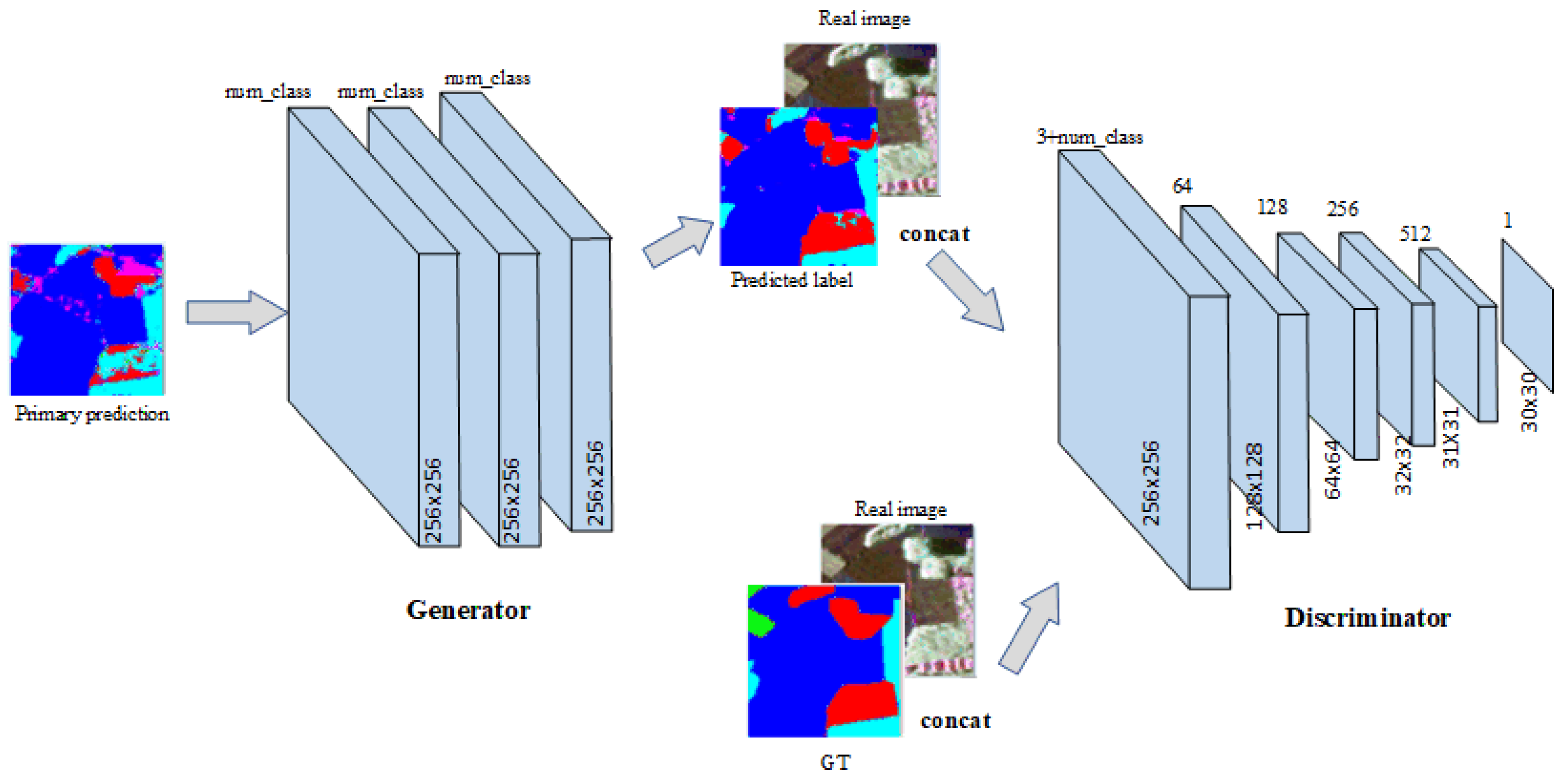
2.3.1. Generative Model

As opposed to other GAN-based segmentation methods, the input of our generator is a primary predicted label image instead of a real image. Therefore, the generator acts as a spatial filter which explores the spatial relationships between labels without changing the size of an image. Considering the role of the generator in adversarial training process, we used three layers of convolution to construct the generator which is illustrated in Figure 4. The first and second layers of convolution were followed by batch normalization [36] and a rectified linear unit (ReLu) [12]. Batch normalization means to perform batch normalizing transformations [36], which are used to regularize the model. The last layer of convolution is connected to a sigmoid function to generate a distribution map for each category. Finally, the predicted label image is obtained by the argmax function. The kernel size of the convolution is 5 × 5, the stride is set to 1, and the padding is set to “same”.

2.3.2. Discriminative Model

The discriminative model plays a central role in GAN. The structure of the discriminator has a great influence on the potential spatial distribution GAN explores. Usually, the discriminator is applied at three levels: pixel, patch, and image. At the pixel level, the discriminative model determines the image pixel by pixel, called PixelGAN. In PixelGAN, the output size of the discriminator is the same as the input size. At the patch level, the discriminative model makes decisions in K × K patch, called PatchGAN. At the image level, the discriminator judges the image in the image level, called ImageGAN; the output size of the discriminator is 1 × 1.

In the semantic segmentation, the predicted label is not only related to the input pixels but also closely related to the surrounding labels. PatchGAN discriminates the label from a regional perspective, which is more in line with the requirements of semantic segmentation than PixelGAN and ImageGAN. Therefore, the proposed method uses the structure of discriminator like the PatchGAN. The architecture of the discriminator is demonstrated in Figure 4.

2.4. Loss Function

For the purpose of improving the accuracy of segmentation and the stability of training, it is essential to choose a reasonable loss function. The loss function of the proposed method is made up of two parts: a loss function of the prior network—FCN, and a loss function of the likelihood network—GAN. Cross-entropy loss is used as the loss of prior network expressed as:

$$l_p(x,y)=-\frac{1}{n}\sum _{i=1}^{n}fcn\left(x_i\right)\log y_i,$$

(3)

where y${}_i$ is the probability distribution of the ground truth, and fcn(x${}_i$) is the probability distribution of the label image predicted by FCN. In addition, x represents the input real image. The loss function of GAN can be denoted as:

$$\underset{G}{min}\underset{D}{max}V(G,D)=E_{x\sim p_{data}\left(x\right)}\left[\log D\left(x\right)\right]+E_{z\sim p_z\left(z\right)}\left[\log (1-D\left(G\left(z\right)\right))\right],$$

(4)

where G and D are denoted as generators and discriminators, respectively. In many GAN-based segmentation models, the loss function of the discriminative network can generally be given by:

$$d_{loss}=\frac{1}{n}\sum _{i=1}^n(-\log (predict\_rea{l}_i)+\log (1-predict\_fak{e}_i\left)\right),$$

(5)

where predict_real${}_i$ is the output of the discriminator when the input is ground truth, and predict_fake${}_i$ is the output of the discriminator when the input is a primary predicted label image. For the loss function of generative model, named g${}_{loss}$, researchers usually use different strategies. In pix2pix, g${}_{loss}$ contains an L1 loss term and an adversarial loss term g${}_{GAN}$. The L1 loss term, which is used to make the predicted label graph closer to the ground truth, can be expressed as:

$$L_1=\frac{1}{n}\sum _{i=1}^{n}abs(outpu{t}_i-g{t}_i),$$

(6)

where output${}_i$ is the label image predicted by the generator and gt${}_i$ is the ground truth. Moreover, the term abs means to take the absolute value of the amount in the associated brackets. In the paper [35], g${}_{loss}$ contains a cross-entropy loss term, an L1 loss term, and an adversarial loss term g${}_{GAN}$. From Equations (3) and (6), it can be found that the L1 loss calculates the absolute difference between the labels, and the cross-entropy is the degree of correlation between the label probabilities. Therefore, L1 loss is more appropriate to tasks such as color conversion, and cross-entropy loss is more suitable for semantic segmentation tasks. The loss function of the generative model of the proposed approach is defined as:

$$g_{loss}={\lambda }_1{\mathrm{g}}_{\mathrm{GAN}}+{\lambda }_2{\mathrm{g}}_{cross-entropy}={\lambda }_1(\frac{1}{n}\sum _{i=1}^n\log (-predict\_fak{e}_i)+{\lambda }_2(-\frac{1}{n}\sum _{i=1}^{n}gan\left(x_i\right)\log y_i),$$

(7)

where ${\lambda }_1$ and ${\lambda }_2$ represent weighting coefficients (${\lambda }_1$ + ${\lambda }_2$ = 1), and gan(x${}_i$) is the probability distribution of the label image predicted by the generator. The remaining parameters are consistent with those in Equations (3) and (5).

3. Flowchart and Setting

The flowchart of the proposed method for training and testing processes is illustrated in Figure 5. Figure 5a demonstrates the training process for the proposed network. The entire training network comprises three parts: the FCN, the generator, and the discriminator. Firstly, the training image is input to the FCN module, and after passing through the multi-layer fully convolutional network, a preliminary predicted label image is obtained. The loss of this module is acquired by calculating the cross entropy between the preliminary predicted label and the ground truth. Secondly, the preliminary predicted image is taken as an input and optimized by the generator to obtain a predicted label image. The generator is equivalent to a spatial filter that provides some necessary spatial information without changing the image size. Then, in order to take advantage of spatial information, the real training image is concatenated with the predicted label and ground truth respectively to use as the input of discriminator. The discriminator module performs true and false identification of the input. The adversarial loss is calculated by discriminating the ground truth as true and discriminating the predicted label as false. At the same time, the adversarial loss and cross-entropy loss are back-propagated by gradient descent, and the entire network’s parameters are continually updated until the training process is completed. Figure 5b demonstrates the testing process of the network. In comparison with the training network, the testing network is relatively simple, because the testing process does not need to update the parameters of the network, and also does not require the discriminative model to perform true or false discrimination. Therefore, the testing process is divided into two modules: the FCN module and the generator module. The input test image is initially extracted by the FCN module and further optimized by the generator module. And then a final segmentation result is produced.

As shown in Figure 1, the framework used for segmentation is composed of an FCN module and a GAN module. The detailed structure of the FCN can be clearly seen in Figure 3. The values of the relevant parameters are set according to the flow of implementation. The learning rate is set to 0.00001 and the batch size is set to 10. Figure 4 shows the structure of the GAN module. The ${\lambda }_1$ and ${\lambda }_2$ in Section 2.4 are set to 0.8 and 0.2, respectively. In addition, momentum parameter is set to 0.5, and the exponential moving average is set to 0.99.

4. Experiment

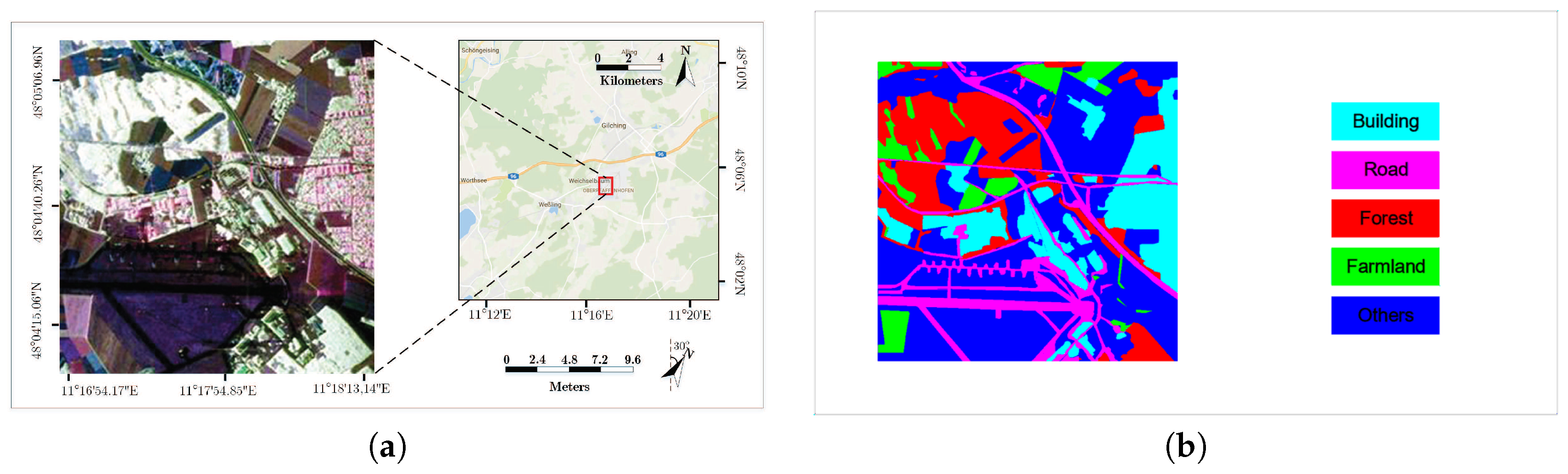
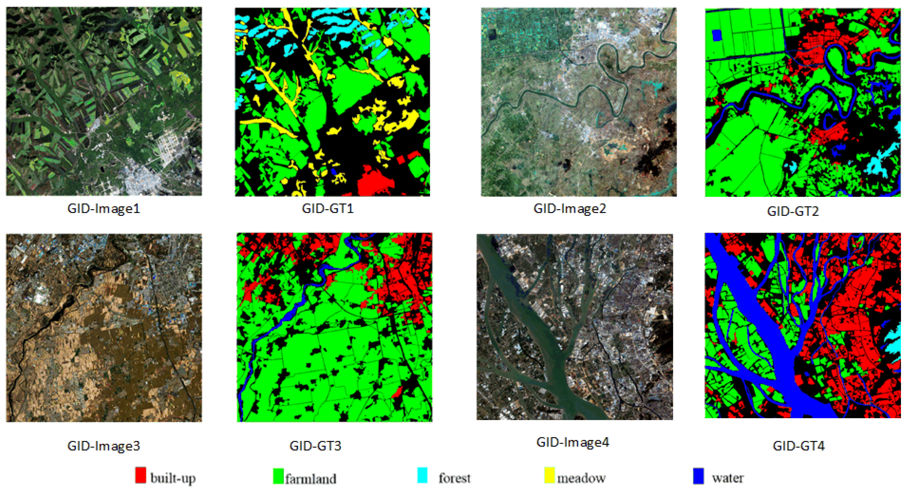
4.1. Experiment Data

To assess the performance of the proposed semantic segmentation method, some experiments were performed on ESAR and Gaofen Image Dataset (GID) [37] images. (1) The first dataset is ESAR data. As displayed in Figure 6a, the ESAR image which was acquired in Germany, has a spatial resolution of 3 × 2.2 m and a dimension of $1300\times 1200$ pixels. The ground truth of the ESAR image is shown in Figure 6b, which contains five categories: road, farmland, building, forest, and other land cover. To test the segmentation effect of the algorithm, the image was divided into four pieces, three of which were used as training sets and the rest of which were used as test sets. Each piece was cut into 100 small 256 × 256 images with a sampling interval of 49 pixels. In order to obtain the entire image of segmentation result, we needed to test each of the different pieces separately. Therefore, we used the four image pieces for four different training and testing sessions. Since training images are limited, like the papers [38,39,40], we did not set up a validation set to ensure adequate training data; (2) The second dataset was GID, which is a high-resolution dataset for land pixel level classification. It contains 150 high-resolution Gaofen-2 (GF-2) images acquired from more than 60 different cities in China [37] from 5 December 2014 to 13 October 2016. Five interested categories are labeled in different colors: built-up (red), farmland (green), forest (cyan), meadow (yellow), and water area (blue). Areas that do not fall into the above five categories or that cannot be artificially identified are marked in black. Figure 7 shows some examples of the original image and the corresponding ground truth. In dataset 2, the size of each image is 6800 × 7200. We randomly selected 120 images as the training set, 15 as the test set, and the final 15 as the validation set. Each large image was cut into 256 × 256 small images without overlap. During the test, these 256 × 256 small images were input into the trained model to obtain the predicted label images, and then the predicted label images were stitched into corresponding full-size images, the original style.

4.2. Experiment Results

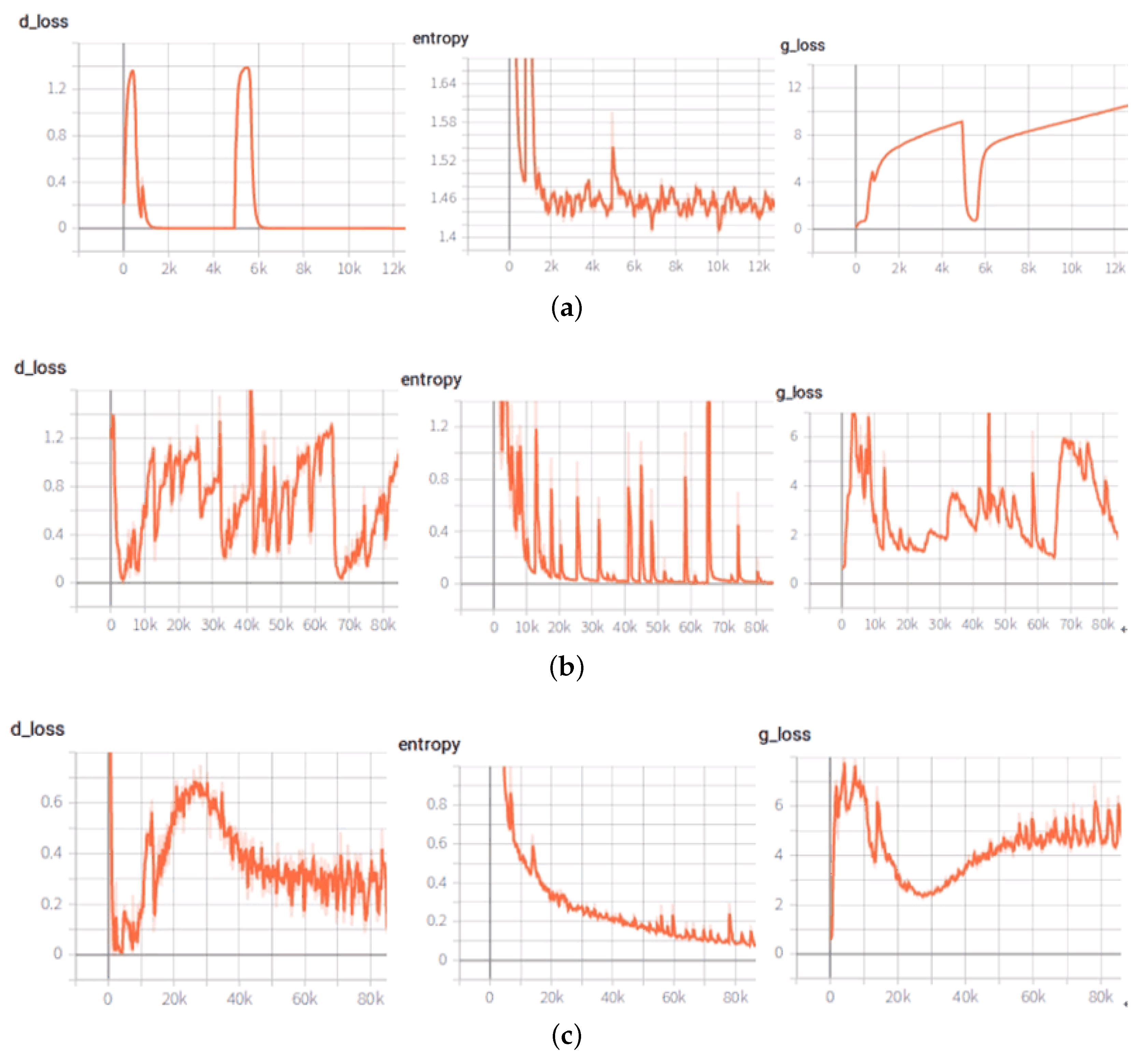
4.2.1. Training Stability Comparison

In order to verify the stability of the proposed method in training, we compared it with other GAN-based segmentation methods, such as pix2pix [30] and CRFAS [35]. Since the other GAN-based methods did not make much difference in training, we only listed the comparison with pix2pix. For the convenience of comparison, we added an observation—cross-entropy loss—which did not participate in the training of pix2pix. After many experiments, we found that the training of pix2pix was not stable. In some cases, pix2pix converged to a local optimum, causing cross-entropy loss to converge to a larger value, which is shown in Figure 8a. In some other cases, pix2pix normally converged, as shown in Figure 8b. However, there was a large amplitude of cross-entropy loss. In the proposed method, the cross-entropy loss in the prior network(FCN) guides the training of the likelihood network (GAN). Figure 8c demonstrates the training state of our proposed method. It can be found that the cross-entropy loss drops steadily and eventually converges, and the loss of GAN also converges steadily.

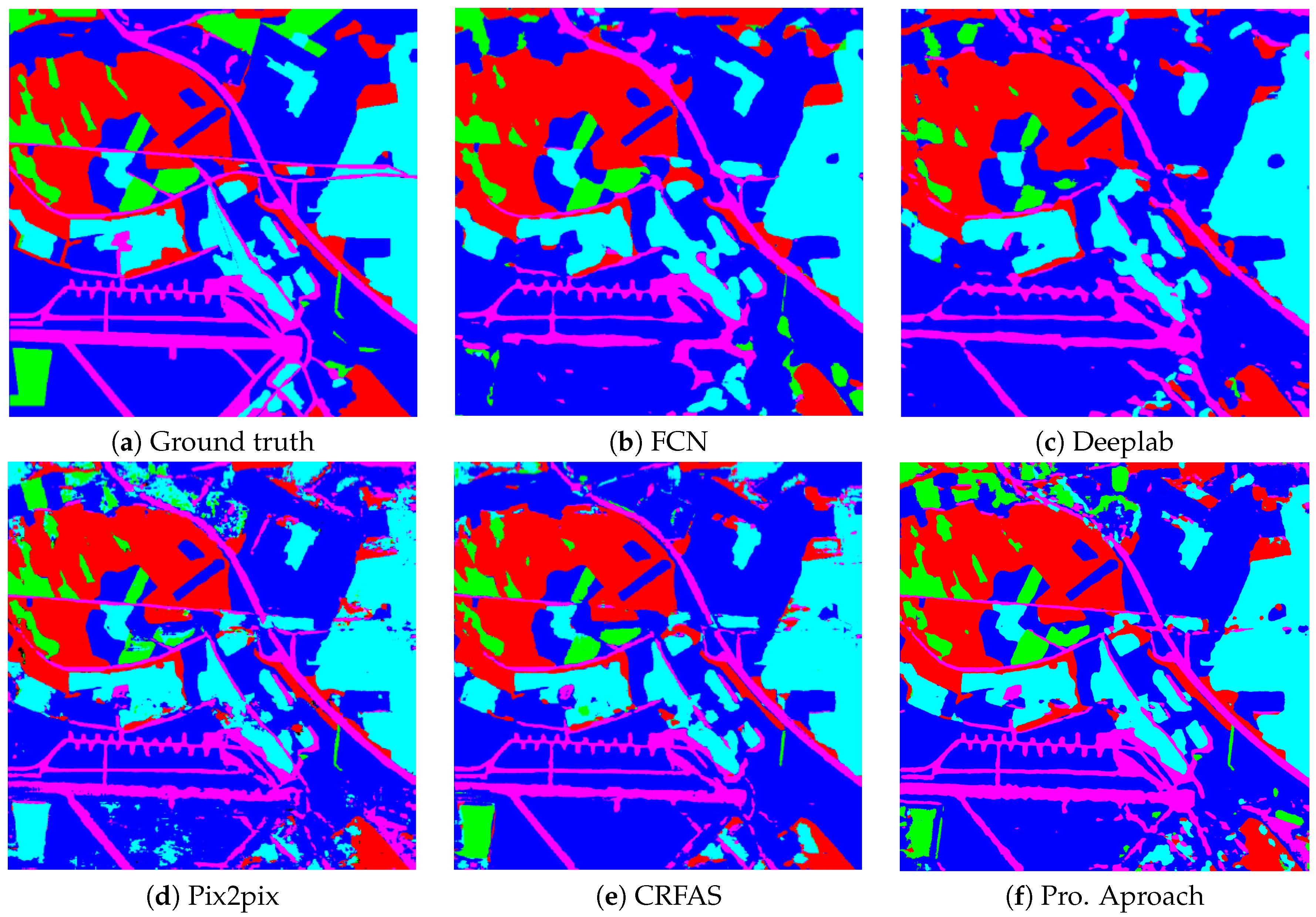
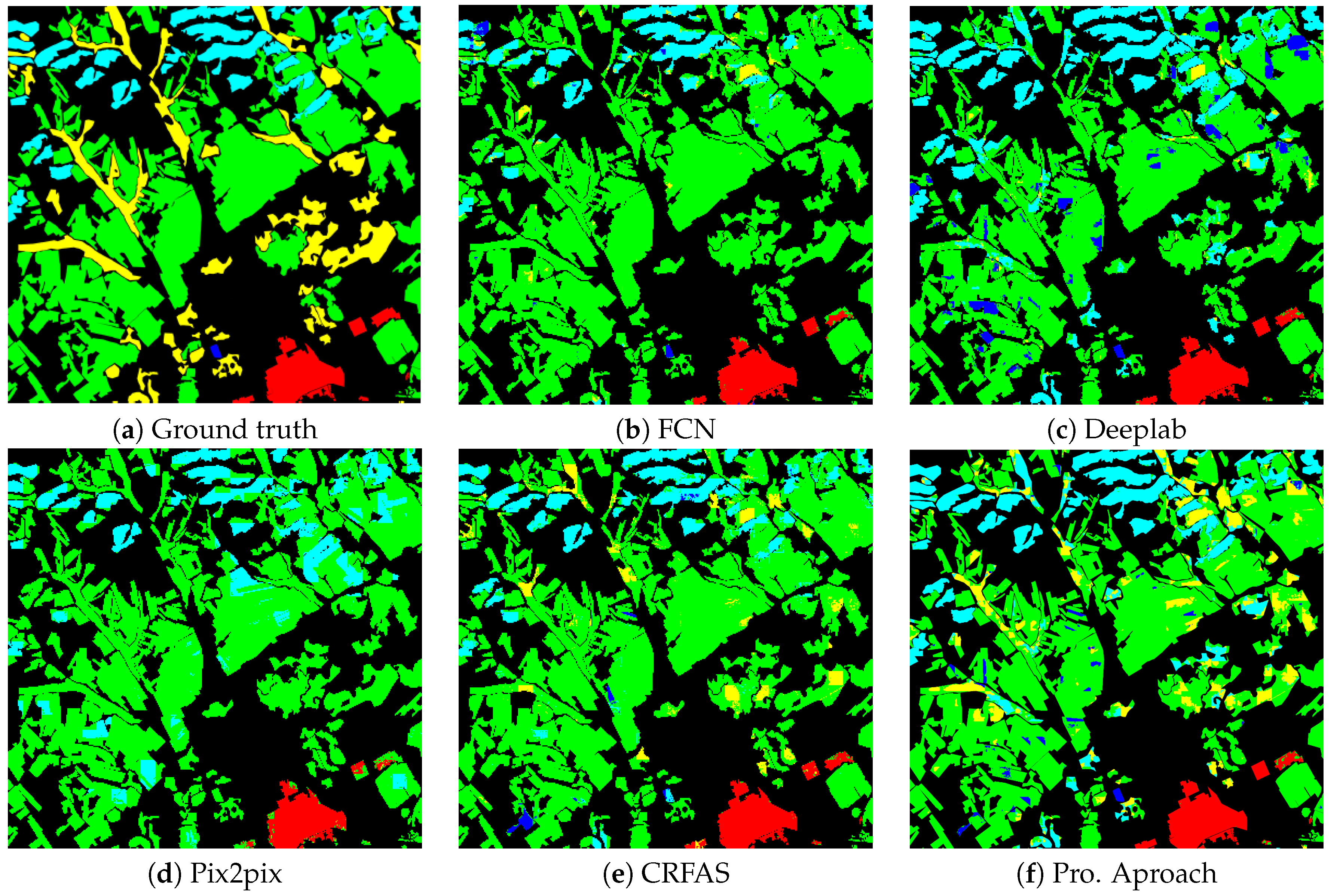
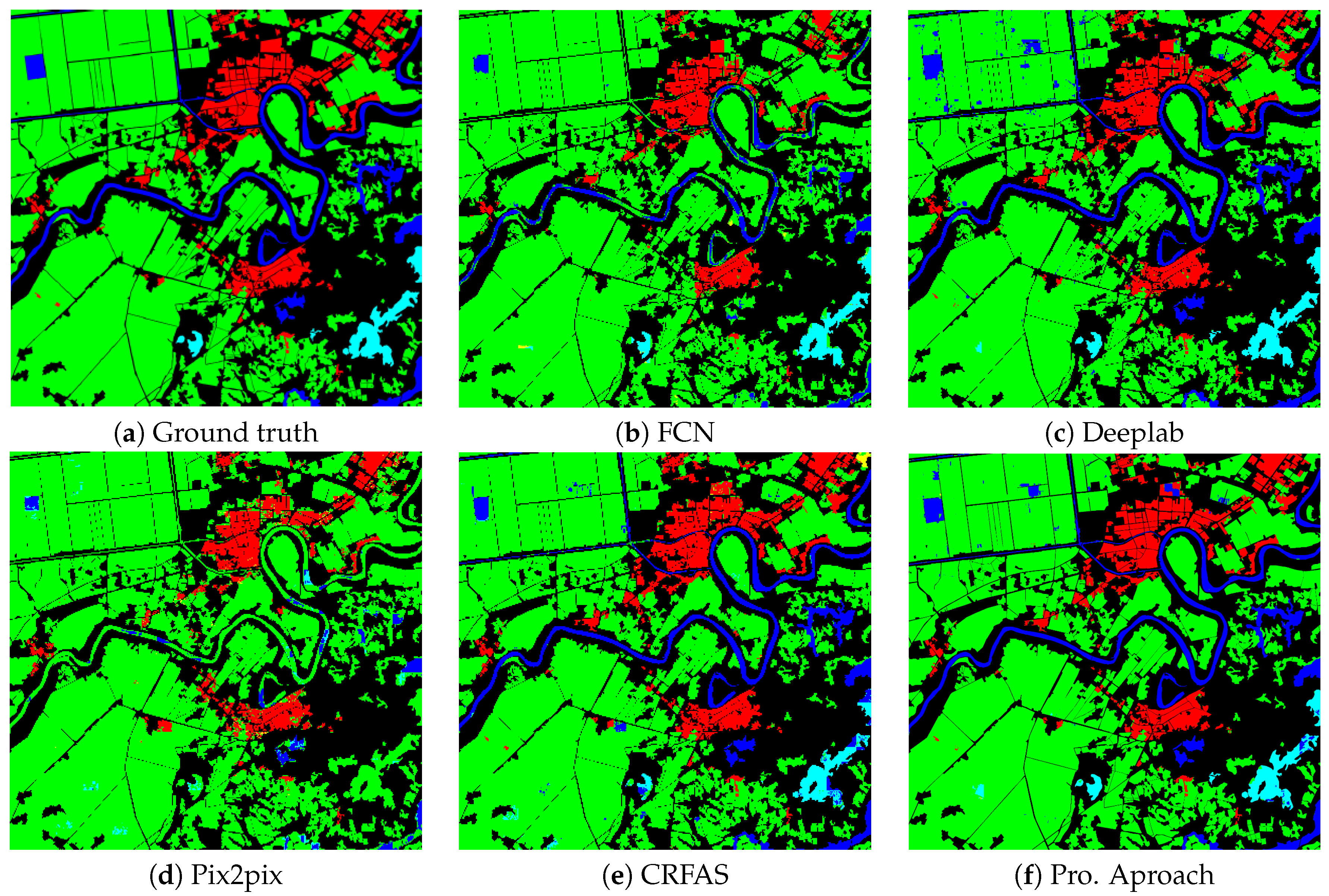
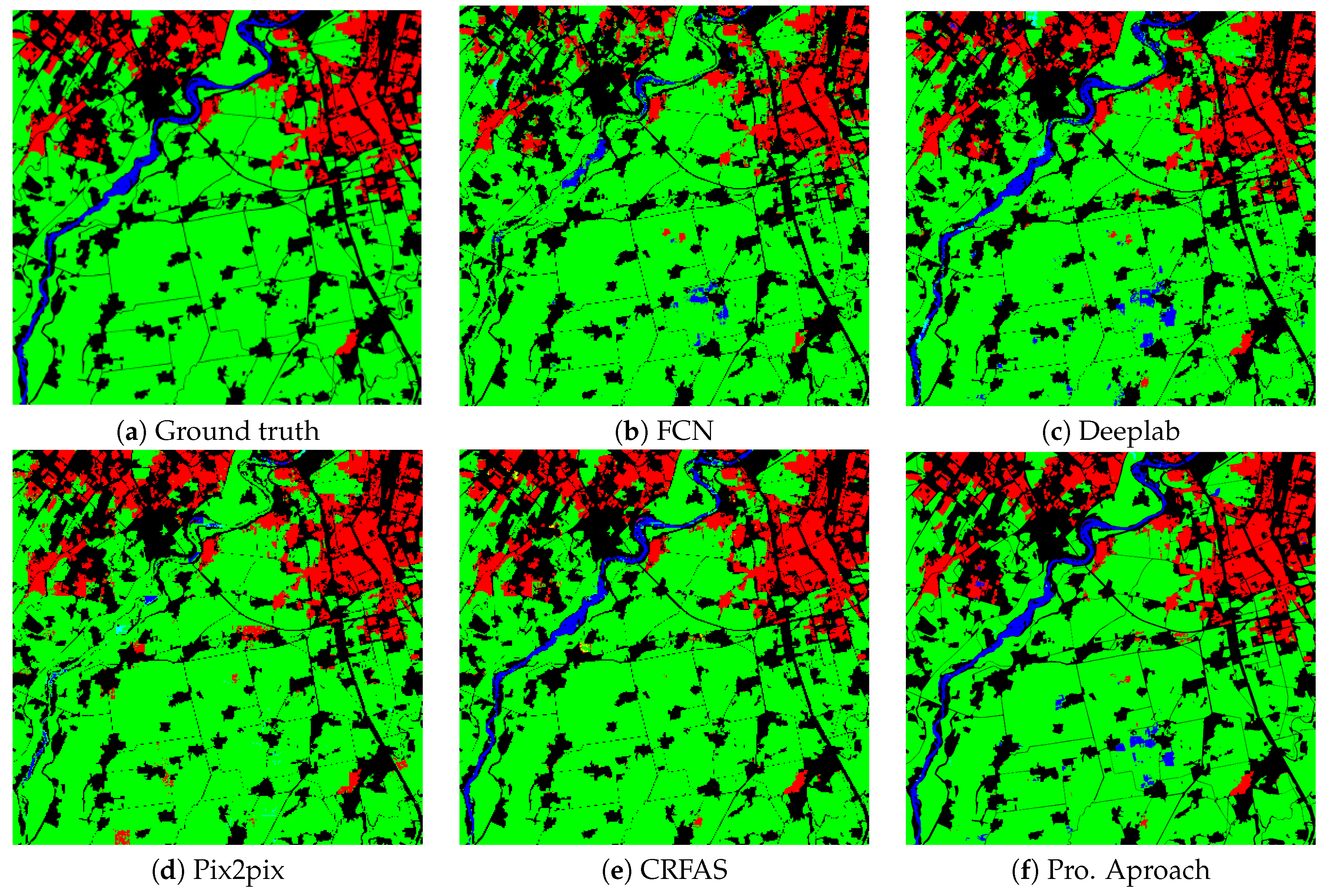
4.2.2. Segmentation Results

In order to verify the advantages of the proposed method in segmentation, four other methods, namely, FCN, Deeplab, pix2pix, and CRFAS, were used for comparison. FCN was the first comparison algorithm, which is used as the prior network in the proposed method and widely used as a benchmark for segmentation. The second comparison algorithm was Deeplab, since it essentially optimizes the results of the FCN using CRF, which is similar to the proposed approach. For the third segmentation algorithm, pix2pix was used—a typical GAN-based approach. CRFAS is a Bayesian segmentation method based on GAN, which is our previous work.

Figure 9 qualitatively illustrates the segmentation results of five different algorithms on ESAR. Three examples of the segmentation results conducted on experiment data2 with the five methods are demonstrated in Figure 10, Figure 11 and Figure 12. GID-image 1, 2, and 3 contain 5, 4, and 3 labels, respectively.

For the ESAR data, the proposed method achieved a good segmentation result, as shown in Figure 9. Compared with other methods, only the proposed method effectively distinguishes the farmland class (green) in the upper left corner of the image. Since the category represented by blue, others, is difficult to determine, the proposed method does not have much of an advantage than other methods. For the GID dataset, the proposed method also achieved good segmentation results, as shown in Figure 10, Figure 11 and Figure 12. Figure 10 illustrates that the proposed approach obtains the best segmentation result for the yellow category (meadow).

For the quantitative assessment of the proposed method, the following three evaluation parameters were adopted: (1) The confusion matrix and average accuracy; (2) F1 score; (3) Mean Intersection over Union (MIoU).

Table 1. Confusion matrix for ESAR data.

Method	Category	Farmland	Forest	Others	Road	Building	Average
FCN	Farmland	0.4617	0.0897	0.3863	0.0216	0.0407	0.8183
	Forest	0.0167	0.8756	0.0390	0.0125	0.0562
	Others	0.0433	0.0135	0.8751	0.0387	0.0295
	Road	0.490	0.0208	0.2858	0.5934	0.0509
	Building	0.0004	0.0228	0.0461	0.0108	0.9199
Deeplab	Farmland	0.4503	0.2191	0.3143	0.0039	0.0124	0.8387
	Forest	0.0074	0.8901	0.0514	0.0161	0.0350
	Others	0.0164	0.0116	0.9226	0.0327	0.0166
	Road	0.0087	0.0419	0.3430	0.5509	0.0509
	Building	0.0004	0.0228	0.0461	0.0108	0.9448
Pix2pix	Farmland	0.3588	0.0623	0.2377	0.0255	0.3156	0.8243
	Forest	0.0206	0.8430	0.0505	0.0221	0.0638
	Others	0.0218	0.0061	0.8802	0.0479	0.0440
	Road	0.0028	0.0087	0.2002	0.7500	0.0383
	Building	0.0042	0.0275	0.0541	0.0181	0.8962
CRFAS	Farmland	0.4781	0.0970	0.2306	0.0277	0.1515	0.8474
	Forest	0.0127	0.8351	0.0506	0.0229	0.0786
	Others	0.0222	0.0093	0.9373	0.0312	0.0001
	Road	0.0067	0.0245	0.2342	0.6879	0.0467
	Building	0.0047	0.0371	0.0489	0.0222	0.8870
Pro. Aproach	Farmland	0.5861	0.2346	0.1487	0.0203	0.0103	0.8648
	Forest	0.0442	0.8864	0.0123	0.0409	0.0162
	Others	0.0086	0.0278	0.9123	0.0089	0.0424
	Road	0.0064	0.1592	0.0204	0.7715	0.0425
	Building	0.0007	0.0312	0.0175	0.0109	0.9397

,

Table 2. Confusion matrix for GID-image1.

Method	Category	Farmland	Water	Building	Meadow	Forest	Average
FCN	Farmland	0.9839	0.0008	0.0001	0.0127	0.0025	0.7631
	Water	0.2499	0.7501	0.0000	0.0000	0.0000
	Building	0.0640	0.0011	0.9349	0.0000	0.0000
	Meadow	0.9871	0.0006	0.0000	0.0064	0.0059
	Forest	0.3137	0.0224	0.0000	0.0349	0.6290
Deeplab	Farmland	0.9310	0.0502	0.000	0.0077	0.0111	0.7799
	Water	0.0048	0.9947	0.0000	0.0000	0.0004
	Building	0.0213	0.0000	0.9787	0.0000	0.0000
	Meadow	0.6742	0.0034	0.0000	0.0329	0.2895
	Forest	0.0042	0.0000	0.0000	0.0000	0.9958
Pix2pix	Farmland	0.9153	0.0000	0.0000	0.0000	0.847	0.7178
	Water	1.0000	0.0000	0.0000	0.0000	0.0000
	Building	0.1352	0.0000	0.8546	0.0101	0.0000
	Meadow	0.9831	0.0000	0.0000	0.0000	0.0169
	Forest	0.3265	0.0000	0.0000	0.0000	0.6735
CRFAS	Farmland	0.9569	0.0071	0.0000	0.0261	0.0099	0.7827
	Water	0.0082	0.2857	0.0000	0.0000	0.7061
	Building	0.0165	0.0000	0.9710	0.0125	0.0000
	Meadow	0.8544	0.0004	0.0000	0.1121	0.0332
	Forest	0.2200	0.0081	0.0000	0.0006	0.7713
Pro. Aproach	Farmland	0.9211	0.0169	0.0000	0.0590	0.0030	0.8160
	Water	0.0034	0.9966	0.0000	0.0000	0.0000
	Building	0.0184	0.0000	0.9816	0.0000	0.0000
	Meadow	0.4844	0.0029	0.0000	0.2917	0.2210
	Forest	0.0132	0.0000	0.0000	0.0001	0.9867

,

Table 3. Confusion matrix for GID-image2.

Method	Category	Farmland	Water	Building	Meadow	Forest	Average
FCN	Farmland	0.9969	0.0006	0.0009	0.0120	0.0004	0.9245
	Water	0.5007	0.4922	0.0069	0.0002	0.0002
	Building	0.3320	0.0010	0.6667	0.0000	0.0003
	Meadow	0.0000	0.0000	0.0000	0.0000	0.0000
	Forest	0.1373	0.0006	0.0015	0.0071	0.8535
Deeplab	Farmland	0.9891	0.0101	0.002	0.0000	0.0006	0.9803
	Water	0.0138	0.9857	0.0004	0.0000	0.0000
	Building	0.0918	0.0062	0.9020	0.0000	0.0000
	Meadow	0.0000	0.0000	0.0000	0.0000	0.0000
	Forest	0.0014	0.0008	0.0000	0.0000	0.9978
Pix2pix	Farmland	0.9899	0.0003	0.0070	0.0004	0.0025	0.8827
	Water	0.7370	0.2045	0.0062	0.0003	0.0519
	Building	0.2900	0.0000	0.6996	0.0204	0.0000
	Meadow	0.0000	0.0000	0.0000	0.0000	0.0000
	Forest	0.9656	0.0000	0.0000	0.0000	0.0344
CRFAS	Farmland	0.9926	0.0033	0.0008	0.0014	0.0019	0.9817
	Water	0.0336	0.9616	0.0004	0.0000	0.0044
	Building	0.0383	0.0000	0.9596	0.0021	0.0000
	Meadow	0.0000	0.0000	0.0000	0.0000	0.0000
	Forest	0.0727	0.1828	0.0000	0.0006	0.7445
Pro. Aproach	Farmland	0.9956	0.0033	0.0003	0.0000	0.0008	0.9887
	Water	0.0058	0.9942	0.0000	0.0000	0.0000
	Building	0.0533	0.0038	0.9429	0.0000	0.0000
	Meadow	0.0000	0.0000	0.0000	0.0000	0.0000
	Forest	0.0238	0.0609	0.0000	0.0000	0.9153

,

Table 4. Confusion matrix for GID-image3.

Method	Category	Farmland	Water	Building	Meadow	Forest	Average
FCN	Farmland	0.9890	0.0050	0.0056	0.0000	0.0004	0.9316
	Water	0.6899	0.3099	0.0000	0.0000	0.0001
	Building	0.2941	0.0040	0.7019	0.0000	0.0001
	Meadow	0.0000	0.0000	0.0000	0.0000	0.0000
	Forest	0.0000	0.0000	0.0000	0.0000	0.0000
Deeplab	Farmland	0.9808	0.0114	0.063	0.0000	0.0015	0.9754
	Water	0.0798	0.8835	0.0000	0.0000	0.0366
	Building	0.0349	0.0053	0.9598	0.0000	0.0000
	Meadow	0.0000	0.0000	0.0000	0.0000	0.0000
	Forest	0.0000	0.0000	0.0000	0.0000	0.0000
Pix2pix	Farmland	0.9783	0.0114	0.0063	0.0000	0.0015	0.9559
	Water	0.7815	0.1436	0.0047	0.0000	0.0701
	Building	0.0386	0.0000	0.9609	0.0005	0.0000
	Meadow	0.0000	0.0000	0.0000	0.0000	0.0000
	Forest	0.0000	0.0000	0.0000	0.0000	0.0000
CRFAS	Farmland	0.9932	0.0000	0.0058	0.0008	0.0001	0.9881
	Water	0.0095	0.8785	0.0009	0.0000	0.0256
	Building	0.0214	0.0003	0.9765	0.0018	0.0000
	Meadow	0.0000	0.0000	0.0000	0.0000	0.0000
	Forest	0.0000	0.0000	0.0000	0.0000	0.0000
Pro. Aproach	Farmland	0.9864	0.0065	0.0071	0.0000	0.0000	0.9851
	Water	0.0102	0.9897	0.0000	0.0000	0.0000
	Building	0.00217	0.0019	0.9764	0.00000	0.0001
	Meadow	0.0000	0.0000	0.0000	0.0000	0.0000
	Forest	0.0000	0.0000	0.0000	0.0000	0.0000

and

Table 5. Confusion matrix for GID.

Method	Category	Farmland	Water	Building	Meadow	Forest	Average
FCN	Farmland	0.9399	0.0042	0.0493	0.0022	0.0044	0.8711
	Water	0.2568	0.7238	0.0116	0.0007	0.0071
	Building	0.1905	0.0065	0.7995	0.0002	0.0033
	Meadow	0.9871	0.0006	0.0000	0.0064	0.0059
	Forest	0.5022	0.0088	0.0011	0.0434	0.4445
Deeplab	Farmland	0.9534	0.0180	0.0232	0.0004	0.0049	0.9238
	Water	0.1198	0.8774	0.0013	0	0.0015
	Building	0.0465	0.0026	0.9502	0	0.0007
	Meadow	0.6741	0.0034	0	0.0330	0.2894
	Forest	0.3131	0.0629	0.0008	0.0370	0.5862
Pix2pix	Farmland	0.9443	0.0017	0.0318	0.0034	0.0187	0.8704
	Water	0.2189	0.7440	0.0039	0.0001	0.0331
	Building	0.1851	0.0013	0.8044	0.0091	0.0001
	Meadow	0.9831	0	0	0	0.0169
	Forest	0.8250	0.0004	0	0	0.1750
CRFAS	Farmland	0.9773	0.0030	0.0103	0.0043	0.0050	0.9414
	Water	0.0630	0.9275	0.0021	0.0004	0.0070
	Building	0.0443	0.0007	0.9522	0.0027	0
	Meadow	0.8543	0.0004	0	0.1121	0.0332
	Forest	0.6464	0.0131	0.0012	0.0011	0.3383
Pro. Aproach	Farmland	0.9690	0.0065	0.0195	0.0020	0.0030	0.9483
	Water	0.1288	0.8691	0.0007	0.0002	0.0012
	Building	0.0255	0.0023	0.9720	0.00000	0.0002
	Meadow	0.7478	0.0082	0.0000	0.0651	0.1789
	Forest	0.1486	0.0064	0.0007	0.0008	0.8435

list the confusion matrixes of the segmentation results, where correct and average accuracy is marked in bold. For the ESAR data, the average accuracy of the proposed approach was the highest, 4.65% higher than FCN, 2.61% higher than Deeplab, 4.05% higher than pix2pix, and 1.74% higher than CRFAS, as shown in Table 1. For the GID dataset, the proposed method also achieved the highest average accuracy. It can be seen from Table 5 that the average accuracy of the proposed method was 7.72%, 2.45%, 7.79%, and 0.69% higher than FCN, Deeplab, pix2pix, and CRFAS, respectively. In addition, a similar conclusion can be obtained from one single GID image, as shown in Table 2, Table 3 and Table 4. The proposed method utilizes FCN as the prior network, and then uses GAN to optimize the results of the prior network. So it is reasonable that the segmentation accuracy of the proposed method was higher than FCN. Compared to Deeplab, the proposed algorithm uses GAN instead of CRF to explore the potential spatial relationship between labels. In the two experimental datasets, the proposed method achieves better segmentation than Deeplab. In the GAN-based segmentation method, the proposed algorithm has certain advantages in segmentation accuracy compared to pix2pix and CRFAS.

The F1 score is an important indicator of semantic segmentation, the calculation of which is based on recall and precision. Equations (8) and (9) give the calculation of the precision and recall, respectively.

$$Precision=\frac{tp}{tp+fp},$$

(8)

$$Recall=\frac{tp}{tp+fn},$$

(9)

where tp represents true positive, which is the amount of pixels in the class for both the predicted result and the real label. fp stands for false positive, which is the number of pixels predicted for each category but not for the real label. fn stands for false negative, which is the number of pixels in each category that are not predicted label but are real label as such. F1 score is an evaluation metric used to balance precision and recall, which is defined as:

$$F1=2·\frac{Precision·Recall}{Precison+Recall}.$$

(10)

The value of F1 score is positively correlated with the segmentation result. The larger the of F1 score, the better the segmentation result is, and vice versa.

Mean intersection over union (MIoU) is a typical measure of semantic segmentation. The calculation of MIoU is given as:

$$MIoU=\frac{1}{k}{\displaystyle \sum _{i=1}^k}\frac{p_{ii}}{{\displaystyle \sum _{j=1}^k}{p}_{ij}+{\displaystyle \sum _{j=1}^k}{p}_{ji}-p_{ii}},$$

(11)

where p${}_{ij}$ denotes the amount of pixels that its real label is made of, i, and the predicted label is j. The value of MIoU is also positively correlated with the segmentation result.

Table 6. F1 score and mean intersection over union (MIoU) of ESAR data.

Data	Method	F1 Score					MIoU
		Farmland	Forest	Others	Road	Building
ESAR	FCN	0.4871	0.8840	0.8558	0.6698	0.8697	0.6270
	Deeplab	0.5634	0.8732	0.8781	0.6489	0.9105	0.6529
	Pix2pix	0.4550	0.8807	0.8707	0.7555	0.8001	0.6266
	CRFAS	0.5717	0.8570	0.9032	0.7349	0.8580	0.6612
	Pro. Aproach	0.6094	0.8915	0.8981	0.7908	0.9097	0.7091

and

Table 7. F1 score and MIoU of GID.

Data	Method	F1 Score					MIoU
		Farmland	Water	Building	Meadow	Forest
GID-image1	FCN	0.8484	0.3413	0.9656	0.0118	0.7617	0.4994
	Deeplab	0.8785	0.0713	0.9892	0.0621	0.7998	0.4995
	Pix2pix	0.8104	0	0.9216	0	0.6239	0.3978
	CRFAS	0.8565	0.1003	0.9849	0.1852	0.8195	0.5137
	Pro. Aproach	0.8923	0.1881	0.9906	0.3898	0.8429	0.5723
GID-image2	FCN	0.9556	0.6560	0.7940	0	0.9130	0.5803
	Deeplab	0.9882	0.9355	0.9472	0	0.9882	0.7464
	Pix2pix	0.9349	0.3385	0.7880	0	0.0530	0.3518
	CRFAS	0.9915	0.9364	0.9760	0	0.8132	0.7004
	Pro. Aproach	0.9940	0.9670	0.9696	0	0.9390	0.7500
GID-image3	FCN	0.9604	0.4106	0.8094	0	0	0.3724
	Deeplab	0.9864	0.7635	0.9615	0	0	0.5032
	Pix2pix	0.9747	0.2496	0.9240	0	0	0.3904
	CRFAS	0.9934	0.9338	0.9715	0	0	0.5615
	Pro. Aproach	0.9912	0.9912	0.8901	0	0	0.5442
GID	FCN	0.9148	0.8247	0.7681	0.0099	0.5521	0.5109
	Deeplab	0.9508	0.8803	0.9141	0.0569	0.6398	0.6068
	Pix2pix	0.9156	0.8479	0.8111	0	0.1925	0.4738
	CRFAS	0.9609	0.9523	0.9471	0.1543	0.4468	0.6209
	Pro. Aproach	0.9578	0.8936	0.9307	0.1077	0.8480	0.6817

list the F1 scores and MIoUs for the ESAR dataset and GID dataset, respectively. For the ESAR dataset, the MIoU of the proposed method is greatly improved compared to the other four methods: 0.0821 higher than FCN, 0.0562 higher than Deeplab, 0.0825 higher than pix2pix, and 0.0479 higher than CRFAS. The F1 score for each category is almost the highest. For the GID dataset, the MIoU of the proposed method also has a significant improvement in the entire GID dataset. Compared to other methods, the F1 score of the proposed method for the "Forest" category is significantly improved.

4.3. Time Consumption

Experiments are performed on four NVIDIA Titan X using Tensorflow.

Table 8. Training time of ESAR dataset.

Method	FCN	Deeplab	pix2pix	CRFAS	Pro. Approach
time(h)	16.9	25.3	26.7	81.2	26.9

lists the training time of ESAR dataset for the five algorithms. Time scale is hour (h). It can been seen that the proposed method is basically equivalent to Deeplab and pix2pix, and is much shorted than CRFAS in training time-consuming. Since the proposed method uses FCN as the prior network, it requires more time to train the network than the FCN.

5. Discussion

In the experiment section, the proposed approach was evaluated from three aspects: stability of training, segmentation results, and time consumption. As shown in Figure 8, guided by the prior network, the training is more stable than pix2pix’s. This is in line with our expectations. From the segmentation results which are listed in Table 1 and Table 5, Table 6 and Table 7, the proposed method clearly achieved the highest overall accuracy, F1 score, and MIoU on both datasets. That all indicates that the proposed method makes better use of spatial information and improves the segmentation effect. In terms of time consumption, although the proposed method is not optimal, it has obvious advantages over CRFAS. To further optimize the segmentation effect and apply the proposed method to practical applications, the following aspects should be considered.

(1)

The proposed approach utilizes the generative adversarial network to explore the potential spatial relationships between labels. The structure of GAN has a great impact on the results of the segmentation. Therefore, building a more reasonable generator and discriminator is the key to further improving the performance of semantic segmentation.

(2)

In the proposed method, FCN plays a crucial role as the prior network. Adequate prior knowledge is the foundation of the Bayesian network. To further improve the segmentation accuracy, FCN can be replaced by other better networks, which can be studied in the subsequent work.

(3)

On the GID dataset, compared to other methods in the experiments, although the proposed approach has obvious advantages on MIoU and achieves the highest average accuracy, the F1 scores for each category are not always the highest. Table 7 shows that CRFAS had higher F1 scores for “Farmland”, “Water”, “Building”, and “Meadow” categories than the proposed method. The confusion matrix of GID shown in Table 5 indicates other categories are most often misclassified as ”Farmland”, and that “Meadow” is not effectively segmented. The reasons for this may be related to the inherent properties of the category. This is a question worthy of further study.

(4)

GAN has a problem of mode collapse during the training process. The proposed method uses the cross-entropy loss to guide the training of GAN to avoid this problem. However, this problem has not been completely resolved. Therefore, it is necessary to conduct more in-depth research from the basic principles of GAN.

(5)

In future work, the proposed method will be extended to the segmentation of PolSAR data by using the covariance matrix $\mathit{C}$ or coherency matrix $\mathit{T}$.

6. Conclusions

This paper has presented an end-to-end Bayesian segmentation network based on a generative adversarial network for remote sensing images. In the proposed algorithm, FCN is used as the prior network to get a rough segmentation result, and GAN is used as the likelihood network to optimize the output of FCN, which implements the derivation of the prior probability and likelihood function to the posterior probability. In addition, the cross-entropy loss of FCN is used a priori to guide the training of GAN to make the network converge to global optimality. The function of GAN is to explore the potential spatial relationship between labels, which makes it equivalent to a teachable spatial filter. The effectiveness of the proposed method for semantic segmentation was verified by experiments on ESAR data and GID data. The proposed method outperformed FCN in terms of MIoU by 0.0821 and 0.1708 on two datasets, respectively, and achieved the highest accuracy, F1 score, and MIoU. In terms of time consumption, the proposed method is comparable to pix2pix and Deeplab, which is acceptable.

References

1. Oberweger, M.; Wohlhart, P.; Lepetit, V. Hands Deep in Deep Learning for Hand Pose Estimation. arXiv 2015, arXiv:1502.06807. [Google Scholar]
2. Barth, A.; Siegemund, J.; Meißner, A.; Franke, U.; Förstner, W. Probabilistic Multi-class Scene Flow Segmentation for Traffic Scenes. In Proceedings of the Dagm Conference on Pattern Recognition, Darmstadt, Germany, 22–24 September 2010. [Google Scholar]
3. Cordts, M.; Omran, M.; Ramos, S.; Rehfeld, T.; Enzweiler, M.; Benenson, R.; Franke, U.; Roth, S.; Schiele, B. The Cityscapes Dataset for Semantic Urban Scene Understanding. arXiv 2016, arXiv:1604.01685. [Google Scholar]
4. Deren, L.; Guifeng, Z.; Zhaocong, W.; Lina, Y. An edge embedded marker-based watershed algorithm for high spatial resolution remote sensing image segmentation. IEEE Trans. Image Process. 2010, 19, 2781–2787. [Google Scholar] [CrossRef]
5. Zhang, X.; Xiao, P.; Feng, X.; Wang, J.; Zuo, W. Hybrid region merging method for segmentation of high-resolution remote sensing images. ISPRS J. Photogramm. Remote Sens. 2014, 98, 19–28. [Google Scholar] [CrossRef]
6. Nogueira, K.; Miranda, W.O.; Dos Santos, J.A. Improving spatial feature representation from aerial scenes by using convolutional networks. In Proceedings of the 28th SIBGRAPI Conference on Graphics, Patterns and Images, Salvador, Brazil, 26–29 August 2015; pp. 289–296. [Google Scholar]
7. Noh, H.; Hong, S.; Han, B. Learning deconvolution network for semantic segmentation. In Proceedings of the IEEE International Conference on Computer Vision, lSantiago, Chile, 7–13 December 2015; pp. 1520–1528. [Google Scholar]
8. Peng, C.; Zhang, X.; Yu, G.; Luo, G.; Sun, J. Large Kernel Matters–Improve Semantic Segmentation by Global Convolutional Network. In Proceedings of the IEEE Conference on Computer Vision and Pattern Recognition, Honolulu, HI, USA, 21–26 July 2017; pp. 4353–4361. [Google Scholar]
9. Dan, C.C.; Giusti, A.; Gambardella, L.M.; Schmidhuber, J. Deep Neural Networks Segment Neuronal Membranes in Electron Microscopy Images. Adv. Neural Inf. Process. Syst. 2012, 25, 2852–2860. [Google Scholar]
10. Long, J.; Shelhamer, E.; Darrell, T. Fully convolutional networks for semantic segmentation. In Proceedings of the IEEE Conference on Computer Vision and Pattern Recognition, lBoston, MA, USA, 7–12 June 2015; pp. 3431–3440. [Google Scholar]
11. Simonyan, K.; Zisserman, A. Very deep convolutional networks for large-scale image recognition. arXiv 2014, arXiv:1409.1556. [Google Scholar]
12. Krizhevsky, A.; Sutskever, I.; Hinton, G.E. Imagenet classification with deep convolutional neural networks. Adv. Neural Inf. Process. Syst. 2012, 60, 1097–1105. [Google Scholar] [CrossRef]
13. Szegedy, C.; Liu, W.; Jia, Y.; Sermanet, P.; Reed, S.; Anguelov, D.; Erhan, D.; Vanhoucke, V.; Rabinovich, A. Going deeper with convolutions. In Proceedings of the IEEE Conference on Computer Vision and Pattern Recognition, lBoston, MA, USA, 7–12 June 2015; pp. 1–9. [Google Scholar]
14. He, K.; Zhang, X.; Ren, S.; Sun, J. Deep residual learning for image recognition. In Proceedings of the IEEE Conference on Computer Vision and Pattern Recognition, lVegas, NV, USA, 27–30 June 2016; pp. 770–778. [Google Scholar]
15. Ronneberger, O.; Fischer, P.; Brox, T. U-net: Convolutional networks for biomedical image segmentation. In Proceedings of the International Conference on Medical Image Computing and Computer-Assisted Intervention, Munich, Germany, 5–9 October 2015; pp. 234–241. [Google Scholar]
16. Badrinarayanan, V.; Kendall, A.; Cipolla, R. Segnet: A deep convolutional encoder-decoder architecture for image segmentation. IEEE Trans. Pattern Anal. Mach. Intell. 2017, 39, 2481–2495. [Google Scholar] [CrossRef] [PubMed]
17. Chen, L.C.; Papandreou, G.; Kokkinos, I.; Murphy, K.; Yuille, A.L. Deeplab: Semantic image segmentation with deep convolutional nets, atrous convolution, and fully connected crfs. IEEE Trans. Pattern Anal. Mach. Intell. 2017, 40, 834–848. [Google Scholar] [CrossRef]
18. Zhao, H.; Shi, J.; Qi, X.; Wang, X.; Jia, J. Pyramid scene parsing network. In Proceedings of the IEEE Conference on Computer Vision and Pattern Recognition, Honolulu, HI, USA, 21–26 July 2017; pp. 2881–2890. [Google Scholar]
19. Mortensen, E.N.; Jia, J. Real-time semi-automatic segmentation using a Bayesian network. In Proceedings of the IEEE Computer Society Conference on Computer Vision and Pattern Recognition (CVPR’06), New York, NY, USA, 17–22 June 2006; pp. 1007–1014. [Google Scholar]
20. Pelizzari, S.; Bioucas-Dias, J.M. Bayesian Segmentation of Oceanic SAR Images: Application to Oil Spill Detection. arXiv 2010, arXiv:1007.4969. [Google Scholar]
21. Zhang, L.; Ji, Q. A Bayesian network model for automatic and interactive image segmentation. IEEE Trans. Image Process. 2011, 20, 2582–2593. [Google Scholar] [CrossRef] [PubMed] [Green Version]
22. Vezhnevets, A.; Ferrari, V.; Buhmann, J.M. Weakly supervised structured output learning for semantic segmentation. In Proceedings of the IEEE Conference on Computer Vision and Pattern Recognition, Providence, RI, USA, 16–21 June 2012; pp. 845–852. [Google Scholar]
23. Ge, W.; Liu, G. Semantic segmentation based on neural network and Bayesian network. Proc. SPIE 2013, 8917, 89170Z. [Google Scholar]
24. Kendall, A.; Badrinarayanan, V.; Cipolla, R. Bayesian segnet: Model uncertainty in deep convolutional encoder-decoder architectures for scene understanding. arXiv 2015, arXiv:1511.02680. [Google Scholar]
25. Coombes, M.; Eaton, W.; Chen, W.H. Unmanned ground operations using semantic image segmentation through a Bayesian network. In Proceedings of the International Conference on Unmanned Aircraft Systems, Arlington, VA, USA, 7–10 June 2016. [Google Scholar]
26. Wu, F.Y. The potts model. Rev. Mod. Phys. 1982, 54, 235. [Google Scholar] [CrossRef]
27. Goodfellow, I.; Pouget-Abadie, J.; Mirza, M.; Xu, B.; Warde-Farley, D.; Ozair, S.; Courville, A.; Bengio, Y. Generative adversarial nets. In Proceedings of the 27th International Conference on Neural Information Processing Systems, Montreal, QC, Canada, 2 December 2014; Volume 2, pp. 2672–2680. [Google Scholar]
28. Luc, P.; Couprie, C.; Chintala, S.; Verbeek, J. Semantic segmentation using adversarial networks. arXiv 2016, arXiv:1611.08408. [Google Scholar]
29. Zhu, W.; Xiang, X.; Tran, T.D.; Xie, X. Adversarial deep structural networks for mammographic mass segmentation. arXiv 2016, arXiv:1612.05970. [Google Scholar]
30. Isola, P.; Zhu, J.Y.; Zhou, T.; Efros, A.A. Image-to-image translation with conditional adversarial networks. In Proceedings of the IEEE Conference on Computer Vision and Pattern Recognition, Honolulu, HI, USA, 21–26 July 2017; pp. 1125–1134. [Google Scholar]
31. Souly, N.; Spampinato, C.; Shah, M. Semi supervised semantic segmentation using generative adversarial network. In Proceedings of the IEEE International Conference on Computer Vision, Venice, Italy, 22–29 October 2017; pp. 5688–5696. [Google Scholar]
32. Fu, C.; Lee, S.; Joon Ho, D.; Han, S.; Salama, P.; Dunn, K.W.; Delp, E.J. Three dimensional fluorescence microscopy image synthesis and segmentation. In Proceedings of the IEEE Conference on Computer Vision and Pattern Recognition Workshops, Salt Lake City, UT, USA, 18–22 June 2018; pp. 2221–2229. [Google Scholar]
33. Huo, Y.; Xu, Z.; Bao, S.; Bermudez, C.; Plassard, A.J.; Liu, J.; Yao, Y.; Assad, A.; Abramson, R.G.; Landman, B.A. Splenomegaly segmentation using global convolutional kernels and conditional generative adversarial networks. Int. Soc. Opt. Photonics 2018, 10574, 1057409. [Google Scholar]
34. Ma, F.; Gao, F.; Sun, J.; Zhou, H.; Hussain, A. Weakly Supervised Segmentation of SAR Imagery Using Superpixel and Hierarchically Adversarial CRF. Remote Sens. 2019, 11, 512. [Google Scholar] [CrossRef] [Green Version]
35. He, C.; Fang, P.; Zhang, Z.; Xiong, D.; Liao, M. An End-to-End Conditional Random Fields and Skip-Connected Generative Adversarial Segmentation Network for Remote Sensing Images. Remote Sens. 2019, 11, 1604. [Google Scholar] [CrossRef] [Green Version]
36. Ioffe, S.; Szegedy, C. Batch Normalization: Accelerating Deep Network Training by Reducing Internal Covariate Shift. arXiv 2015, arXiv:1502.03167. [Google Scholar]
37. Tong, X.Y.; Xia, G.S.; Lu, Q.; Shen, H.; Li, S.; You, S.; Zhang, L. Land-Cover Classification with High-Resolution Remote Sensing Images Using Transferable Deep Models. Remote Sens. Environ. 2019, 237, 111322. [Google Scholar] [CrossRef] [Green Version]
38. Wei, X.; Guo, Y.; Gao, X.; Yan, M.; Sun, X. A new semantic segmentation model for remote sensing images. In Proceedings of the IEEE International Geoscience and Remote Sensing Symposium (IGARSS), Fort Worth, TX, USA, 23–28 July 2017; pp. 1776–1779. [Google Scholar]
39. Liu, Y.; Fan, B.; Wang, L.; Bai, J.; Xiang, S.; Pan, C. Semantic labeling in very high resolution images via a self-cascaded convolutional neural network. ISPRS J. Photogramm. Remote Sens. 2018, 145, 78–95. [Google Scholar] [CrossRef] [Green Version]
40. Cheng, W.; Yang, W.; Wang, M.; Wang, G.; Chen, J. Context Aggregation Network for Semantic Labeling in Aerial Images. Remote Sens. 2019, 11, 1158. [Google Scholar] [CrossRef] [Green Version]
Figure 1. Bayesian segmentation framework.
Remotesensing 12 00216 g001
Figure 2. Comparison of several segmentation frameworks. (a) Fully convolutional networks make dense predictions for image semantic segmentation. (b) A fully connected conditional random field (CRF) is introduced to Deeplab; The input of the CRF contains the image to be segmented and the final output of the convolutional layer. (c) The network contains a generator and a discriminator. The generator produces label prediction. (d) The proposed method combines FCN and GAN. (bd) can be regarded as Bayesian networks.
Remotesensing 12 00216 g002
Figure 3. Structure of the prior network—FCN, and the flow of implementation. The network first uses a pretrained model VGG19 for feature extraction, and then connects three down-sampling convolutional layers and three up-sampling deconvolution layers.
Remotesensing 12 00216 g003
Figure 4. Structure of the likelihood network-GAN. The generator uses a three-layer convolution, which acts as a learning spatial filter. The discrimination using six-layer convolution is the same as PatchGAN.
Remotesensing 12 00216 g004
Figure 5. Flowchart of training and testing processes. (a) Training process; (b) Testing process.
Remotesensing 12 00216 g005
Figure 6. Experiment data1. (a) The ESAR image data; (b) The ground truth of ESAR image.
Remotesensing 12 00216 g006
Figure 7. Experiment data2.
Remotesensing 12 00216 g007
Figure 8. Training stability comparison. (a) Pix2pix converges to local optimum; (b) Pix2pix converges normally; (c) The training situation of the proposed method.
Remotesensing 12 00216 g008
Figure 9. Segmentation results of the ESAR image. (a) The ground truth; (bd) the results by FCN, Deeplab, and Pix2pix, respectively; (e,f) the results by CRFAS and the proposed approach.
Remotesensing 12 00216 g009
Figure 10. Segmentation results of GID-image1. (a) The ground truth; (bd) the results by FCN, Deeplab, and Pix2pix, respectively; (e,f) the results by CRFAS and the proposed approach.
Remotesensing 12 00216 g010
Figure 11. Segmentation results of GID-image2. (a) The ground truth; (bd) the results by FCN, Deeplab, and Pix2pix, respectively; (e,f) the results by CRFAS and the proposed approach.
Remotesensing 12 00216 g011
Figure 12. Segmentation results of GID-image3. (a) The ground truth; (bd) the results by FCN, Deeplab, and Pix2pix, respectively; (e,f) the results by CRFAS and the proposed approach.
Remotesensing 12 00216 g012