Surface Temperature of the Planet Earth from Satellite Data

Abstract

The Intergovernmental Panel on Climate Change regular scientific assessments of global warming is based on measurements of air temperature from weather stations, buoys or ships. More specifically, air temperature annual means are estimated from their integration into climate models, with some areas (Africa, Antarctica, seas) being clearly underrepresented. Present satellites allow estimation of surface temperature for a full coverage of our planet with a sub-daily revisit frequency and kilometric resolution. In this work, a simple methodology is developed that allows estimating the surface temperature of Planet Earth with MODIS Terra and Aqua land and sea surface temperature products, as if the whole planet was reduced to a single pixel. The results, through a completely independent methodology, corroborate the temperature anomalies retrieved from climate models and show a linear warming trend of 0.018 ± 0.007 °C/yr.

1. Introduction

The Intergovernmental Panel on Climate Change (IPCC) publishes Assessment Reports periodically, with the aim of analyzing the current state of the climate. The IPCC’s Fifth Assessment Report [1] was the last of these reports and provided the scientific input into the Paris Agreement, which aims to strengthen the global response to the threat of climate change by holding the increase in the global average temperature to well below 2 °C above pre-industrial levels and to pursue efforts to limit the temperature increase to 1.5 °C above pre-industrial levels. The reference global temperatures datasets are derived from air temperature in situ data, with various sources, such as ships, drifting buoys or Argo floats [2], in the case of sea and ocean extensions, and permanent ground-based meteorological stations, which typically measure air temperature at 1.5–2 m, [3] on land. These in situ stations do not cover the entire Earth surface, meaning a lack of representative measures from certain areas of the planet [4].

On the other hand, satellite data provide now temporal series of an adequate span for climate analysis independent of the in situ data. After the launch of the Terra platform, on the 18th of December of 1999, and then the Aqua satellite, on the 4th of May of 2002, four daily measures became available from the MODIS instrument for each 1 km by 1 km pixel (at 10:30, 13:30, 22:30, 01:30 nominal time) [5]. Moreover, the international scientific community has developed surface temperature algorithms since the 80s, which are now capable of estimating the surface Earth temperature from satellite-derived data. Studies show global surface temperature (including land and ocean surfaces) estimations with an associated uncertainty between 1 and 2 K [6].

The aim of this study was to determine if remote sensing is able to retrieve reliably our planet surface temperature changes. We used the MODIS Terra and Aqua Sea Surface Temperature (SST) and Land Surface Temperature (LST) products to estimate the Earth Surface Temperature (EST—the surface temperature of Planet Earth including LST and SST observations), which we then compared with the global annual air temperatures estimated by the NOAA’s National Climatic Data Center (NOAA NCDC) [7]. Finally, the different behavior and trend of the surface temperature were analyzed regionally and locally.

2. Materials and Methods

The MODIS Terra and Aqua SST MOD25 and MYD25 products [8] and the LST MOD11C1 and MYD11C1 products [9] have been downloaded for this study. SST products derived from MODIS are developed by the NASA Ocean Biology Processing Group (OBPG) and the MODIS Ocean Team Computing Facility (MOTCF). Calibrating coefficients, which vary in time, are continuously estimated and verified by the Rosenstiel School of Marine and Atmospheric Science (RSMAS) at the University of Miami. The data used in this study (product MOD25 Version 2.0) have been processed by applying the long wave algorithm [10], which considers MODIS 31 and 32 bands.

MODIS SST spatial resolution is 4.63 km, resulting in a global image of 8640 × 4320 pixels. Pixels have been labelled according to their quality. In this study, only SST pixels with an associated QC (Quality Control) value of 0 and 1, meaning good (clear data with associated scan angles less than 55°) and acceptable (good/acceptable data in glint or high scan angle) quality [10], respectively, have been included in estimations. Those pixels in which the atmospheric correction has failed, where cloud or ice have been detected or have not been processed for other reasons, were not included in our computations, and neither was its associated area proportion.

LST products MOD11C1 (Terra) and MYD11C1 (Aqua) at 0.05° resolutions have been used, resulting in a 7200 × 3600 pixel image size. As with the MOD25 product, LST data has been processed using MODIS 31 and 32 bands as input for a long wave split window algorithm. The average LST error product is 1 °C for temperatures in the range from −10 to 50 °C [11]. LST pixels have also been filtered according to quality control tags explained on the product ATBD (Algorithm Theoretical Basis Document), meaning that only the pixels with QC values of 00 and 01 have been considered, ignoring those not produced due to cloud effects or other reasons [12].The accuracy of the MOD11 version 6 LST product has been tested and was found to mostly fall within 1 K [12,13,14], while MOD25 SST product is provided with an error lower than 0.45 K in most cases [10,15].

The NOAA NCDC uses the Merged Land-Ocean Surface Temperature Analysis (MLOST) in its operational and climate assessment activities, integrated by a land and sea air temperature data. The land dataset contains historical records for over 7000 locations worldwide, requiring adjustments in station locations, temperature instrumentation and land use. The source of sea surface temperature of MLOST is the International Comprehensive Ocean-Atmosphere Data Set (ICOADS), consistent on integrated marine meteorological observations, primarily, from ships and buoys. Both LST and SST grids are used to construct a coherent picture of historical temperature variations across the globe since the late nineteenth century [16].

SST and LST global means have been computed from MODIS Terra at 1:30, 13:30 and Aqua at 10:30 and 22:30, using 8-day composite images, according to SST_ij and LST_ij, which the values of SST and LST, respectively, for each pixel (i,j) on a given day of the year (t). Moreover, m is the column pixel dimension and n is, its line dimension; A_ij, is the area of each pixel and A_total is the sum of the area of the pixels considered in the calculation. Therefore, we obtained an LST and an SST value for each 8-day composite image for the whole span of the data (2003–2016).

$$SS{T}_{MODIS}=\left(SS{T}_{mean}^{\left(01:30\right)}+SS{T}_{mean}^{\left(10:30\right)}+SS{T}_{mean}^{\left(13:30\right)}+SS{T}_{mean}^{\left(22:30\right)}\right)/4$$

(1)

$$LS{T}_{MODIS}=\left(LS{T}_{mean}^{\left(01:30\right)}+LS{T}_{mean}^{\left(10:30\right)}+LS{T}_{mean}^{\left(13:30\right)}+LS{T}_{mean}^{\left(22:30\right)}\right)/4$$

(2)

where $SS{T}_{mean}^t$ and $LS{T}_{mean}^t$ are given by:

$$SS{T}_{mean}^t=\frac{1}{A_{total}}{\displaystyle \sum }_{i=1}^{i=n}{\displaystyle \sum }_{j=1}^{j=m}{A}_{ij}SS{T}_{ij}^t$$

(3)

$$LS{T}_{mean}^t=\frac{1}{A_{total}}{\displaystyle \sum }_{i=1}^{i=n}{\displaystyle \sum }_{j=1}^{j=m}{A}_{ij}LS{T}_{ij}^t$$

(4)

In addition, surface temperature has been estimated for the northern (HN) and southern (HS) hemispheres, and for six latitudinal zones: the low latitudes from the Equator to the Tropic of Cancer in the HN and Tropic of Capricorn in the HS (0–23.5°), mid latitudes from the Tropics to the Arctic Circle in the HN and Antarctic Circle in the HS (23.5°–66.5°) and high latitudes from the Arctic and Antarctic Circles to the Poles (66.5°–90°).

Once SST and LST have been estimated, EST has been calculated by weighting both parameters according to the percentage of area covered by sea and land respectively and taking into consideration the different LST and SST image resolution:

$$EST=\left(A^{SST}\times SS{T}_{MODIS}+A^{LST}\times LS{T}_{MODIS}\right)/\left({\mathrm{A}}^{\mathrm{SST}}+{\mathrm{A}}^{\mathrm{LST}}\right)$$

(5)

No gap-filling was carried out for cloud contaminated data. Manual inspection of retrieved SST and LST 8-day averages showed the presence of outliers, which we removed by a classical Z-score approach (all estimates further away than five standard deviations of the mean, calculated from the whole time series—EST, LST and SST—were not considered). We then estimated the annual temperature averages for LST and SST for the period 2003–2016. Trends were retrieved by linear regression. Estimates of Sen slope results led to similar results. Trend significance was estimated with the Mann-Kendall trend test.

3. Results and Discussion

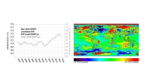
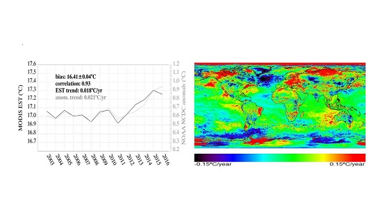
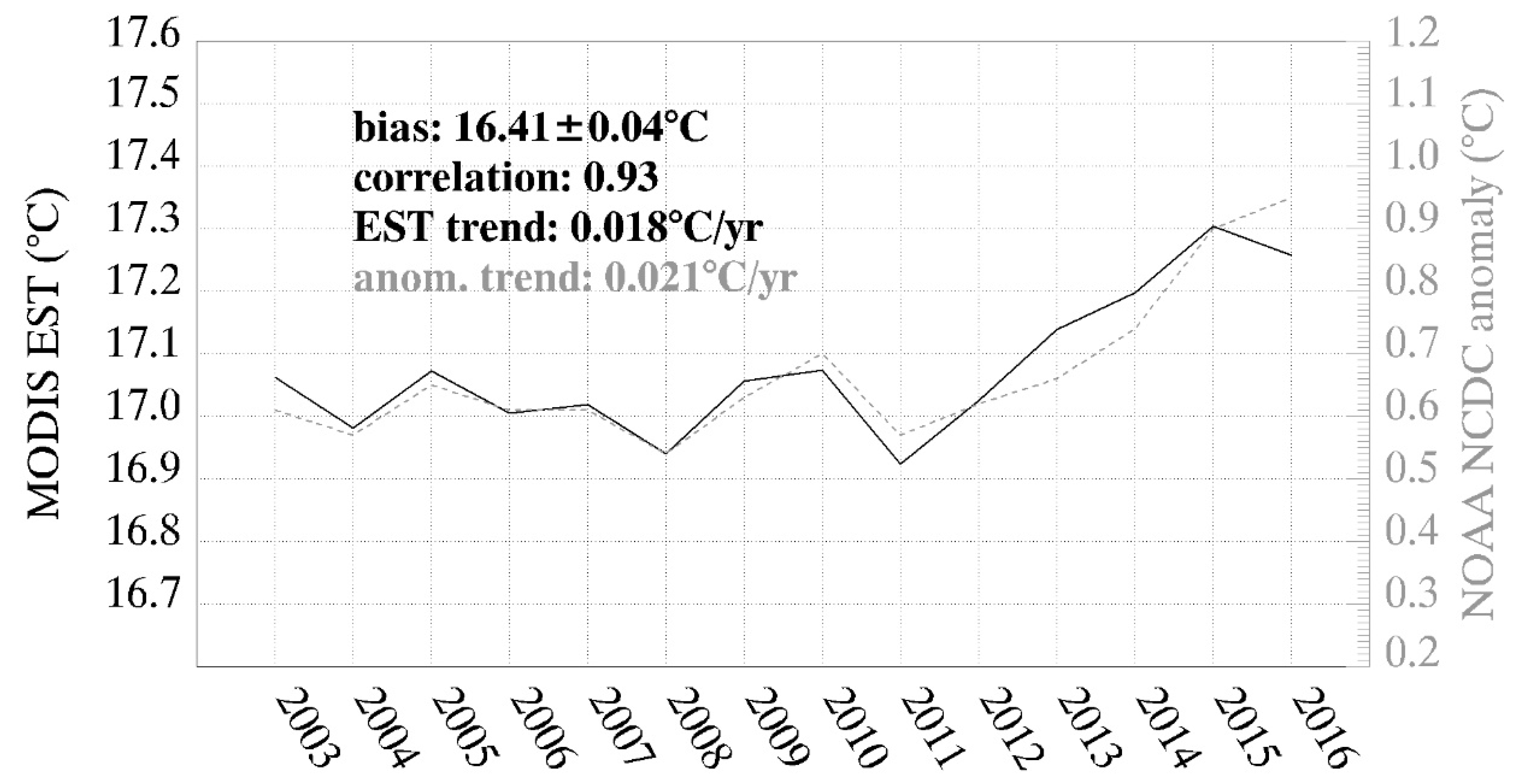
3.1. MODIS Earth Surface Temperature Matches NOAA NCDC Global Air Temperature Estimations

The comparison between the surface temperature values of the Planet Earth obtained from MODIS products (EST) with the methodology developed in this work and the NOAA-NCDC data is shown in Figure 1. We obtain a correlation coefficient of 0.93, with linear trends of 0.018 ±0.007 °C/yr for MODIS EST and 0.021 °C/yr for NOAA NCDC anomalies. The NOAA NCDC anomalies have been calculated by using a reference temperature of 13.9 °C, which is the average combined land and ocean air temperature of the 1901–2000 period [7].The given correlation is statically significant at the 99.9% confidence level, also been estimated by the Sen’s slope method, obtaining 0.018 °C/yr. and a confidence level of 97.5 while the range of differences between the MODIS derived EST and the NOAA NCDC air temperature anomalies is of −0.07 to 0.1 °C and the mean difference for the total period is 0.0043 °C. The median evaluated uncertainty in the period 2003–2016 is 0.10 °C for the SST, 0.20 °C for LST and 0.11 °C for EST. Moreover, trends have also been estimated by the Sen’s slope method, obtaining 0.018 ± 0.007 °C/yr. and a confidence level of 97.5%, strengthening our results.

The high correlation found between the estimations of EST obtained from MODIS products in the present work and the in situ NOAA NCDC database emphasizes the high potential of thermal infrared satellite data as a source of accurate input data of great value for global surface temperature estimates and, therefore, for being applied to climatological studies [17].

Air Temperature Versus Satellite Temperature

We compare two temperature databases, one derived from MODIS Terra and Aqua observations and the other, interpolated from the NOAA NCDC in situ measures. Several differences exist between both types of data sets. First, MODIS satellite observations refer to skin SST while NOAA NCDC measures the air temperature. This fact has been documented to be responsible for a global bias of 1 °C [18].

Cloud coverage affects the information received by thermal sensors, preventing the measure of those pixels situated below clouds and introducing additional biases in respect to air temperature measures. Cloudiness is the main disadvantage that appears when measuring surface temperature with remote sensing sensor: some regions on the planet, such as polar zones are covered by clouds the most part of the year. On the other hand, MODIS allows a continuous, homogenous and global coverage, ensuring four daily representative observations, as previously specified [19]. Despite the more comprehensive data period enabled by AVHRR LST and SST datasets, it has been discarded due to the variability induced by the satellite’s orbital drift [20,21,22].

The wide-scale and periodic observations provided by MODIS are a clear point in favor of satellite estimated surface temperature versus classic air temperature datasets. The second one resides in the global measurement, contrasting with the integration of sparse in situ air temperature measures, not representative on a global scale [19] and which measurements accuracy depend on the sensor characteristics, calibration and exposure. Moreover, the daily air temperature averages only take into consideration the maximum and minimum observations per day. This last consideration leads to errors in the 2–3 °C range, while the level of accurate precision should be 1–2 °C [23].

The aim of this study is not to compare absolute skin and air temperature values, as the existence of biases between both data sets is evident: skin temperature has been documented to be 3 °C lower than air temperature at nighttime [24]. This study neither aims to show local results as several previous studies have done [25,26,27,28,29]. The study shows the potential of satellite thermal observations, represented by MODIS-Terra and MODIS-Aqua, to estimate global surface temperature trends with similar accuracy that the traditional air temperature databases and, therefore, its applicability to climate change studies.

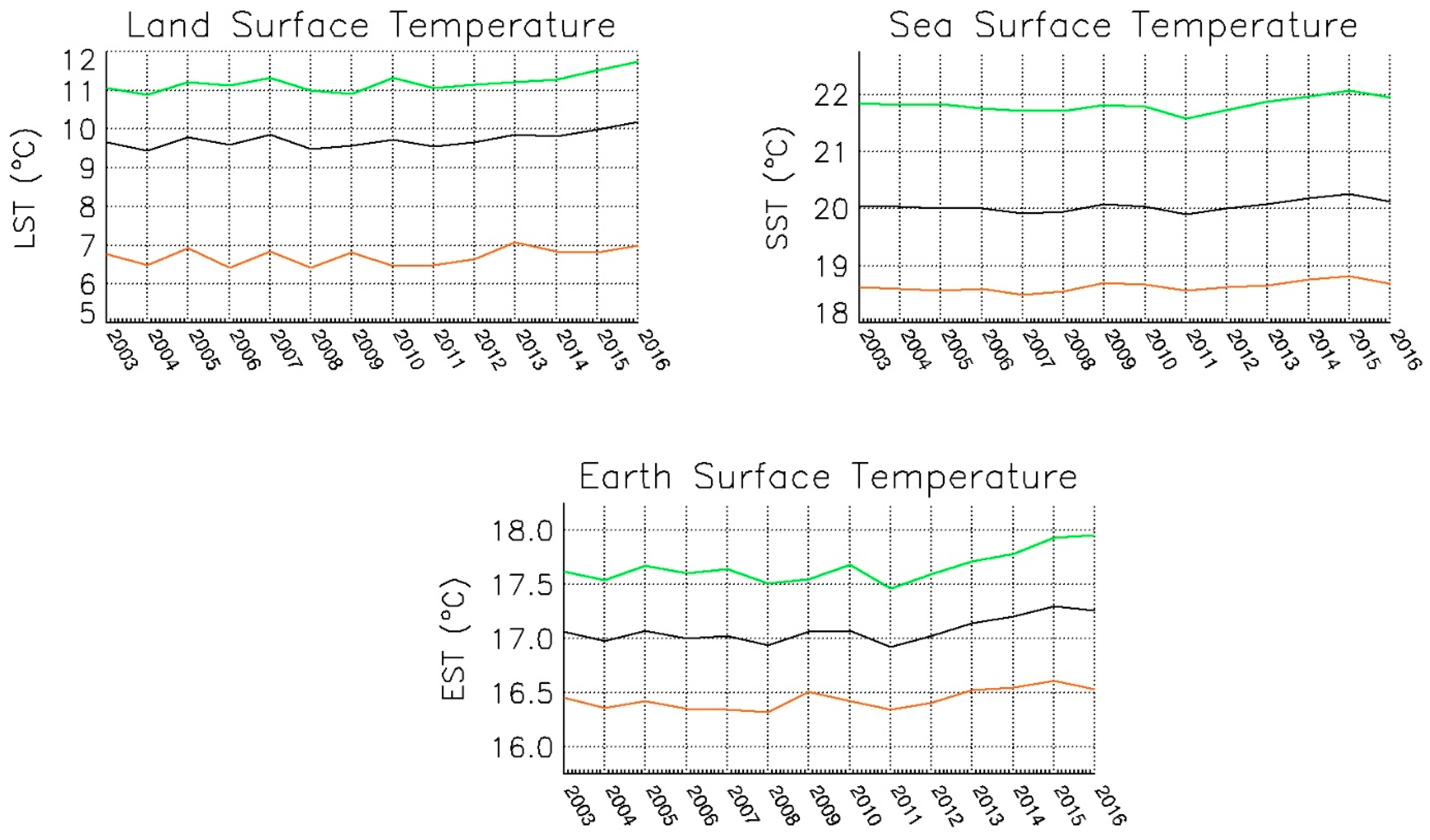
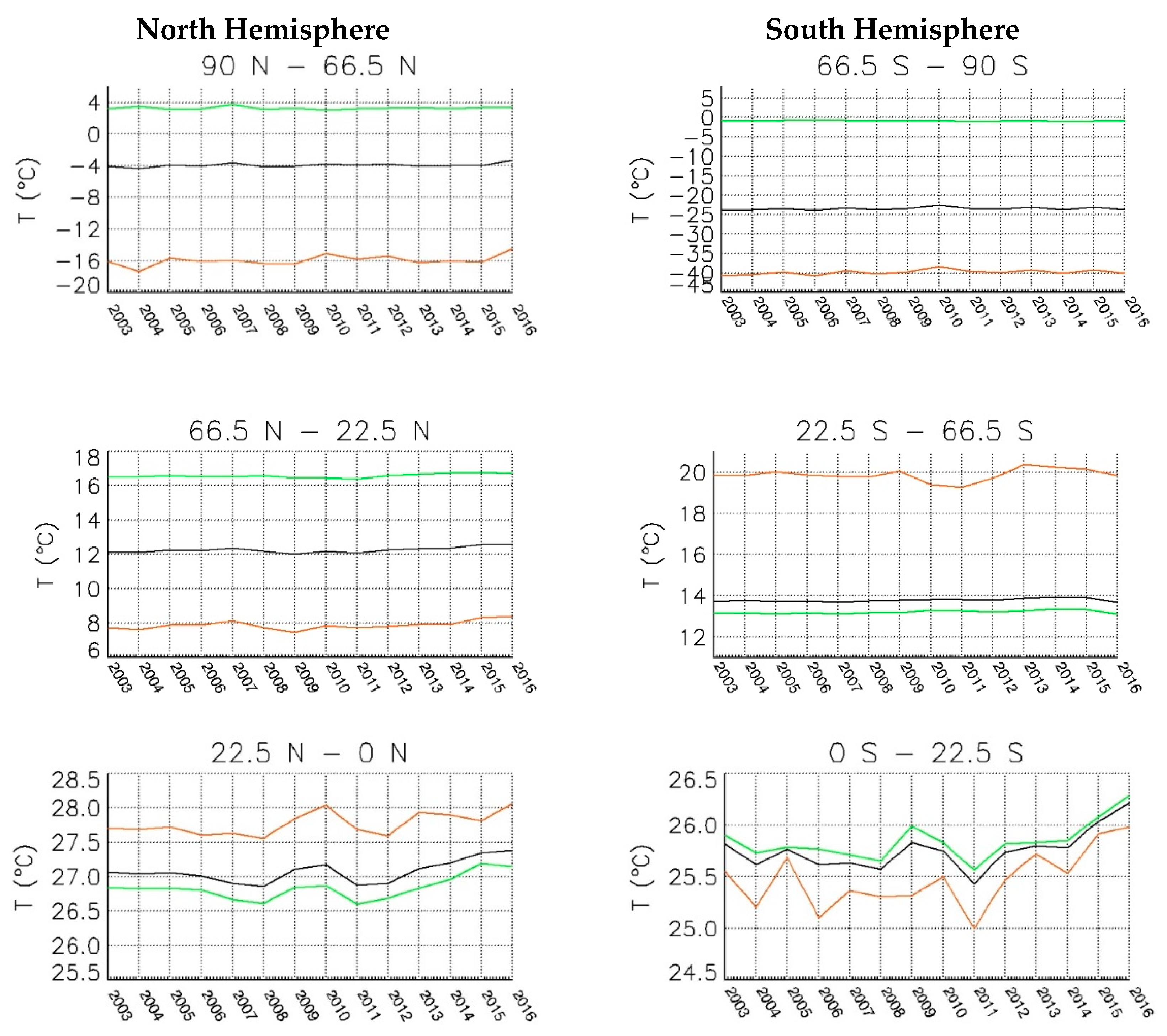
3.2. Regional Analysis: Northern Hemisphere Land Surface Contributes Most to Temperature Increases

The annual values of LST, SST and EST are presented in Figure 2 for the period 2003–2016 by hemisphere and globally. Stability in surface temperatures prevails until 2011, when temperature begins to rise, reaching global peaks in 2015 for SST (20.41 °C) and EST (17.3 °C) and in 2016 for LST (10.18 °C). These 2011–2015/16 variations suppose, in absolute terms, a temperature increase of 0.36, 0.38 and 0.62 °C, respectively. The temperature range of NOAA NCDC global (EST) anomalies during 2011–2016 is 0.38 °C, equal to the estimated in this work from MODIS data.

3.3. High Latitudes Show the Highest Land Surface Temperature Increases

In Figure 3, surface temperature profiles are shown in more detail for the defined six latitudinal zones (high, mid and low). High latitudinal zones, located between 66.5 and 90 degrees and presenting extreme temperatures, only represent 9% of the total surface taken into account, thus they scarcely contribute to global EST. Low latitudes sea surface zones represent 29% of the total surface analyzed in computations, contributing nearly 1/3 of the proportion to the global result. NH low latitudes show an absolute increase of 0.50 °C from 2011 to 2016 and SH low latitudes an increase of 0.78 °C. Several studies relate positive SST anomalies in the eastern Tropical Pacific Ocean with El Niño Southern Oscillation (ENSO) 2015 event [30,31], presenting an associated ONI above 0.5°. Moreover, these SST anomalies are reported to affect the North Atlantic Ocean and the Indian Ocean [32,33], which spread through mid-latitudes. According to our results, sea surface in these mid-latitude zones represents 36% of the data analyzed, contributing more than 1/3 of the proportion of the global results. SST increase during 2011–2016 is quantified as 0.52 °C in the NH mid latitudes, although it is stable in the SH during this period.

Curves associated with SST present a smoother behavior and less variability than LST curves, the sea temperature being less influenced by the summer and winter alternations due to water thermal capacity. The percentage of sea surface is significantly higher than land in the NH low and mid latitudes and the SH low latitudes, thus the final EST curve resembles more the SST behavior than the LST one.

The global EST trend during the period 2003–2016 is 0.018 °C/yr, with high local variability as can be observed in

Table 1. LST, SST and EST linear trends for the 2003–2016 period at a global, hemispherical and latitudinal scale. The LST trend is 0.030 °C/yr., the SST trend is 0.013 °C/yr. and the EST trend is 0.018 °C/yr.

Latitudinal Zone	LST (°C/yr.)	SST (°C/yr.)	EST (°C/yr.)
90°–66.5° NH	0.080	0.0026	0.032
66.5°–23.5° NH	0.036	0.018	0.028
23.5°– 0 NH	0.023	0.021	0.021
0–23.5° SH	0.035	0.022	0.025
23.5°–66.5° SH	0.012	0.010	0.011
66.5°–90° SH	0.064	−0.013	0.031
NH	0.036	0.013	0.022
SH	0.019	0.013	0.014
Global	0.030	0.013	0.018

. By parameter, global trends are of 0.030 °C/yr. for LST and 0.013 °C/yr. for SST. The warming LST trend is not only higher than the SST trend globally, but also for the other nine areas defined. The Copernicus Ocean State Report [34] exhibited an SST warming at a rate of 0.016 °C/yr for the period 1993–2015, meaning a total average increase of 0.4 °C over the considered period, by using satellite-derived ESA Climate Change Initiative (ESA-CCI) observational products Hausfather et al. [35] estimated a 0.12 °C/decade trend from the in situ data set ERSSTv4 for the period 2003–2016. Lawrence et al. [36] used AVHRR data, obtaining a 0.09 °C/decade trend for the period 1985–2000.

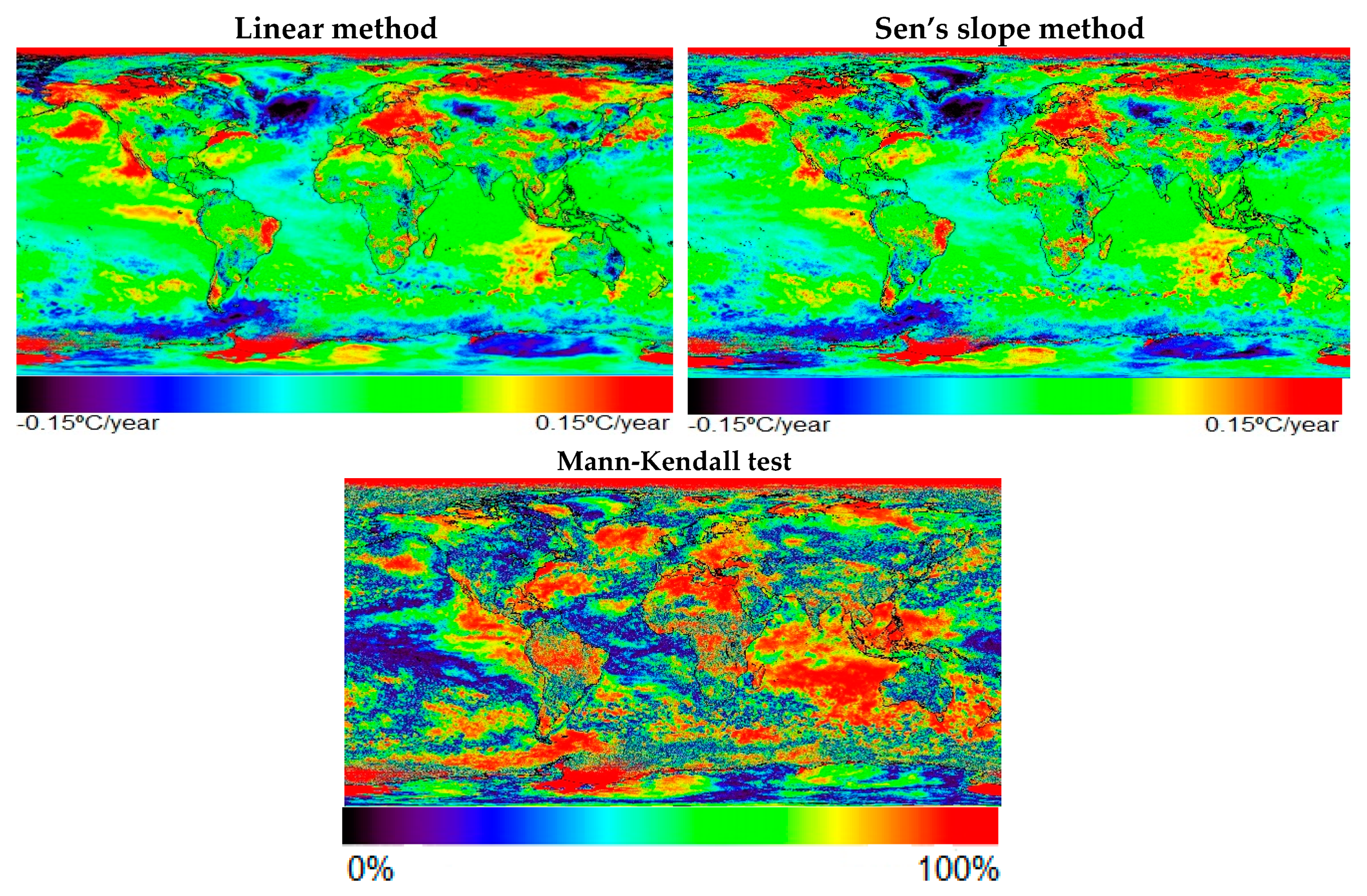
3.4. Local Analysis: Northern Atlantic Ocean Is Cooling Fast, While SIBERIA and Boreal America Is Heating Faster

Linear trends have been estimated by individual parameters, SST and LST, and for our estimated EST at global, hemispherical and latitudinal scales. In the case of SSTs, negative trends are mainly observed in the North Atlantic Ocean, South of Greenland, in the North Pacific, the Sea of Japan, the Yellow Sea and in the Southern Ocean. On the other hand, positive trends are irregularly distributed along NH low and mid-latitudes and in the Atlantic and Pacific Oceans, next to the North American and Australian Continent and the Arctic [37]. In the SH, comprehensive stable areas are observed, with positive trends in the South Pacific, Indian and Atlantic Oceans, in agreement with the results shown in the regional SST analysis of the Fifth IPCC Assessment Report, which establishes an SST increase during 1950–2009 of 0.027 °C/decade, 0.10 °C/decade and 0.063 °C/decade, respectively. For LST, positive trends are found for vast areas of Central and Eastern Europe, Scandinavia and Siberia. In the American Continent, warming trends appear in large areas of Alaska and Canada, between the peninsulas of California and Florida, and in northeastern Brazil and Patagonia. Negative trends appear mainly in the Indian Peninsula and in eastern lengths of Antarctica (Figure 4). Retamales et al. [38] found a negative LST trend in eastern Antarctica of about −1 K/decade, using the MODIS LST product between years 2000–2018. They also estimated the trend with the ERA datasets, obtaining a warming trend of 0.7 K/decade, in disagreement with the results offered by the MODIS LST estimation. The differences between both results show the influence of cloudiness in satellite observations. In particular, cloud coverage increases during winter in this area of the planet, a fact which can impact the calculated temperature trends. The global EST trend has also been estimated by the Theil-Sen method, showing a warming rate of 0.017 °C/yr. with a 97.5% Mann-Kendal significance (Figure 4). Results show the same warming/cooling patterns as estimated by the linear method.

4. Conclusions

The comparison between the planetary MODIS Earth Surface Temperature (EST) presented in this work and the NOAA-NCDC air temperature data shows a correlation coefficient of 0.93 between the two databases, demonstrating the high potential of thermal infrared satellite data to provide accurate data for climatic and meteorological studies. Satellite data are essential in the monitoring of SST, LST and EST (always considering the presence of cloud coverage) as a solid source of continuous data in space and time. In this way, the randomness and lack of data in certain regions of the planet, when referring to in situ data, is widely solved.

The global EST trend is 0.018 °C/yr. The highest EST trend has been computed for the North Hemisphere high latitudes, 0.032 °C/yr., as well as the highest LST trend, 0.080 °C/yr. On the other hand, the highest SST trend is associated to the South Hemisphere low latitudes: 0.022 °C/yr. Globally, SST trends (0.013 °C/yr.) are lower than LST trends (0.030 °C/yr.). SST shows less variability in time than LST and a higher influence on EST, especially in southern latitudes, in which the sea surface extension dominates over the land surface extension. In summary, this paper pretends to open a reflection in the scientific community, covering not only the trends observed from satellites but also the current estimations of air temperature, as well as the validation of both in situ and satellite data. We propose to use the satellite data to estimate anomalies of the average temperature of the Earth’s surface: the thermal data from the satellites could be a proxy to be included in the IPCC assessment reports. Further work should be done in the future, as the extension of MODIS surface temperature temporal series is enlarged with time.

References

1. Field, C.B.; Barros, V.R.; Dokken, D.J.; Mach, K.J.; Mastrandrea, M.D.; Bilir, T.E.; Chatterjee, M.; Ebi, K.L.; Estrada, Y.O.; Genova, R.C.; et al. (Eds.) Climate Change 2014: Impacts, Adaptation, and Vulnerability. Part A: Global and Sectoral Aspects. Contribution of Working Group II to the Fifth Assessment Report of the Intergovernmental Panel on Climate Change; Cambridge University Press: Cambridge, UK; New York, NY, USA, 2014; p. 1132. [Google Scholar]
2. CERSAT. Sea Surface Temperature In Situ Data. Available online: http://cersat.ifremer.fr/data/tools-and-services/match-up-databases/item/298-sea-surface-temperature-in-situ-data (accessed on 5 September 2019).
3. Copernicus. In Situ Observations. Available online: https://insitu.copernicus.eu/observations (accessed on 5 September 2019).
4. Mao, K.B.; Ma, Y.; Tan, X.L.; Shen, X.Y.; Liu, G.; Li, Z.L.; Chen, J.M.; Xia, L. Global surface temperature change analysis based on MODIS data in recent twelve years. Adv. Space Res. 2017, 59, 503–551. [Google Scholar] [CrossRef] [Green Version]
5. NASA. Modis Specifications. Available online: https://modis.gsfc.nasa.gov/about/specifications.php (accessed on 4 June 2019).
6. Wan, Z. New refinements and validation of the collection-6 MODIS land-surface temperature/emissivity product. Remote Sens. Environ. 2014, 140, 36–45. [Google Scholar] [CrossRef]
7. NOAA National Centers for Environmental Information, State of the Climate: Global Climate Report for Annual 2018. Available online: https://www.ncdc.noaa.gov/sotc/global/201813 (accessed on 3 April 2019).
8. Physical Oceanography Distributed Active Archive Center (PO.DAAC). Firefox ESR v38.4.0. Web Page. NASA EOSDIS PO.DAAC, Pasadena, CA. 2018. Available online: https://podaac.jpl.nasa.gov/ (accessed on 5 January 2019).
9. Land Processes Distributed Active Archive Center (LP DAAC). NASA EOSDIC LP.DAAC, Sioux Falls, South Dakota. 2018. Available online: https://lpdaac.isgs.gov/ (accessed on 5 January 2019).
10. Brown, B.; Minnett, P.J. MODIS Infrared Sea Surface Temperature Algorithm. Algorithm Theoretical Basis Document; Version 2.0; University of Miami: Miami, FL, USA, 1999. [Google Scholar]
11. Wan, Z.; Zhang, Y.; Zhang, Q.; Li, Z.-L. Quality assessment and validation of the MODIS global land surface temperature. Int. J. Remote Sens. 2004, 25, 261–274. [Google Scholar] [CrossRef]
12. Wan, Z. Collection-6. MODIS Land Surface Temperature Products Users’ Guide; ERI, University of California: Santa Barbara, CA, USA, 2013. [Google Scholar]
13. Wan, Z. New refinements and validation of the MODIS Land-Surface Temperature/Emissivity products. Remote Sens. Environ. 2008, 112, 59–74. [Google Scholar] [CrossRef]
14. Skokovic, D. Calibration and Validation of Thermal Infrared Remote Sensing Sensors and Land/Sea Surface Temperature algorithms over the Iberian Peninsula. Ph.D. Thesis, University of Valencia, Valencia, Spain, 2017; p. 98. [Google Scholar]
15. Ghanea, M.; Moradi, M.; Kabiri, K.; Mehdinia, A. Investigation and validation of MODIS SST in the northern Persian Gulf. Adv. Space Res. 2016, 57, 127–136. [Google Scholar] [CrossRef]
16. Vose, R.S.; Arndt, D.; Banzon, V.F.; Easterling, D.R.; Gleason, B.; Huang, B.; Kearns, E.; Lawrimore, J.H.; Menne, M.J.; Peterson, T.C. NOAA’s Merged Land-Ocean Surface Temperature Analysis. Bull. Am. Meteorol. Soc. 2012, 93, 1677–1685. [Google Scholar] [CrossRef]
17. Merchant, C.J.; Embury, O.; Bulgin, C.E.; Block, T.; Corlett, G.K.; Fiedler, E.; Good, S.A.; Mittaz, J.; Rayner, N.A.; Berry, D.; et al. Satellite-based time-series of sea-surface temperature since 1981 for climate applications. Sci. Data 2019, 6, 223. [Google Scholar] [CrossRef] [PubMed] [Green Version]
18. Jim, M.; Dickinson, R.E.; Vogelmann, A.M. A comnparison of CCM2-BATS Skin Temperature and Surface-Air Temperature with Satellite and Surface Observations. Am. Meteorol. Soc. 1997, 10, 1505–1524. [Google Scholar]
19. Hooker, J.; Duveiller, G.; Cescatti, A. A global dataset of air temperature derived from satellite remote sensing and weather stations. Sci. Data 2018, 5, 180246. [Google Scholar] [CrossRef] [Green Version]
20. Price, J.C. Using spatial context in satellite data to infer regional scale evapotranspiration. IEEE Trans. Geosci. Remote Sens. 28, 940–948. [CrossRef] [Green Version]
21. Julien, Y.; Sobrino, J.A. Correcting Long Term Data Record V3 estimated LST from orbital drift effects. Remote Sens. Environ. 2012, 123, 207–219. [Google Scholar] [CrossRef]
22. Sobrino, J.A.; Julien, Y.; Atitar, M.; Nerry, F. NOAA-AVHRR orbital drift correction from solar zenithal angle data. IEEE Trans. Geosci. Remote sens. 2008, 46, 4014–4019. [Google Scholar] [CrossRef]
23. Vogt, J.V.; Viau, A.A.; Paquet, A.F. Mapping regional air temperature fields using satellite-derived surface skin temperatures. Int. J. Climatol. 1997, 17, 1559–1579. [Google Scholar] [CrossRef]
24. Alfieri, S.M.; de Lorenzi, F.; Menenti, M. Mapping air temperature using time series analysis of LST: The SINTESI approach. Nonlinear Process. Geophys. 2013, 20, 513–527. [Google Scholar] [CrossRef] [Green Version]
25. Jin, M.; Dickinson, R.E. A generalized algorithm for retrieving cloudy sky skin temperature from satellite thermal infrared radiances. J. Geophys. Res. 2000, 105, 27037–27047. [Google Scholar] [CrossRef]
26. Mildrexler, D.J.; Zhao, M.; Running, S.W. A global comparison between station air temperatures and MODIS land surface temperatures reveals the cooling role of forests. J. Geophys. Res. 2011, 116. [Google Scholar] [CrossRef]
27. Prihodko, L.; Goward, S.N. Estimation of air temperature from remotely sensed surface observations. Remote Sens. Environ. 1997, 60, 335–346. [Google Scholar] [CrossRef]
28. Urban, M.; Eberle, J.; Hüttich, C.; Schmullius, C.; Herold, M. Comparison of satellite-derived land surface temperature and air temperature from meteorological stations on the pan-arctic scale. Remote Sens. 2013, 5, 2348–2367. [Google Scholar] [CrossRef] [Green Version]
29. Jin, M.; Dickinson, R. Land surface skin temperature climatology: Benefitting from the strengths of satellite observations. Environ. Res. Lett. 2010, 5, 044004. [Google Scholar] [CrossRef] [Green Version]
30. Benali, A.; Carvalho, A.C.; Nunes, J.P.; Carvalhais, N.; Santos, A. Estimating air surface temperature in Portugal using MODIS LST data. Remote Sens. Environ. 2012, 124, 108–121. [Google Scholar] [CrossRef]
31. Hameed, S.N.; Jin, D.; Thilakan, V. A model for super El Niños. Nat. Commun. 2018, 9, 2528. [Google Scholar] [CrossRef] [PubMed]
32. Klein, S.A.; Soden, B.J.; Lau, N. Remote Sea Surface Temperature Variations during ENSO: Evidence for a Tropical Atmospheric Bridge. J. Clim. 1999, 12, 917–932. [Google Scholar] [CrossRef] [Green Version]
33. Yang, Y.; Xie, S.-P.; Wu, L.; Yu, K.; Li, J. ENSO forced and local variability of North Tropical Atlantic SST: Model simulations and biases. Clim. Dyn. 2018, 51, 4511–4524. [Google Scholar] [CrossRef]
34. Von Schuckmann, K.; Le Traon, P.Y.; Alvarez-Fanjul, E.; Axell, L.; Balmaseda, M.; Breivik, L.A.; Brewin, R.J.; Bricaud, C.; Drevillon, M.; Drillet, Y.; et al. The Copernicus Marine Environment Monitoring Service Ocean State Report. J. Oper. Oceanogr. 2016, 9, 235–320. [Google Scholar] [CrossRef]
35. Hausfather, Z.; Cowtan, K.; Clarke, D.C.; Jacobs, P.; Richardson, M.; Rohde, R. Assessing recent warming using instrumentally homogenous sea surface temperature records. Sci. Adv. 2017, 3, e1601207. [Google Scholar] [CrossRef] [Green Version]
36. Lawrence, S.P.; Llewelyn-Jones, D.T.; Smith, S.J. The measurement of climate change using data from the Advanced Very High Resolution and Along Track Scanning Radiometers. J. Geophys. Res. 2004, 109, C08017. [Google Scholar] [CrossRef] [Green Version]
37. Von Schuckmann, K.; Le Traon, P.Y.; Smith, N.; Pascual, A.; Djavidnia, S.; Gattuso, J.P.; Grégoire, M.; Nolan, G.; Aaboe, S.; Aguiar, E.; et al. Copernicus Marine Service Ocean State Report, Issue 3. J. Oper. Oceanogr. 2019, 12, 1–23. [Google Scholar] [CrossRef]
38. Retamales-Muñoz, G.; Durán-Alarcón, C.; Mattar, C. Recent land Surface temperature patterns in Antarctica using satellite and reanalysis data. J. S. Am. Earth Sci. 2019, 95, 102304. [Google Scholar] [CrossRef]
Figure 1. MODIS EST absolute temperature versus NOAA-NCDC anomalies. Both datasets estimate positive global surface temperature trends, which are, respectivaly 0.018 °C/yr. for MODIS EST and 0.021 °C/yr. for NOAA NCDC and their correlation coefficient is 0.93.
Remotesensing 12 00218 g001
Figure 2. LST, SST and EST evolution in the NH (green) and SH (orange) and global (black) from 2003 to 2016. Notice how the highest temperatures are obtained for the EST, LST and SST in the NH and the lowest for the SH. Temperature keeps stable until year 2011, when a significant increase is observed from 2011 onwards.
Remotesensing 12 00218 g002
Figure 3. Latitudinal SST (green), LST (orange) and EST (black) evolution in the period 2003–2016. Differences between the three parameters increases with latitude.
Remotesensing 12 00218 g003
Figure 4. Global linear trend map for the period 2003–2016 estimated by the linear (left) and Sen’s slope (right) methods, with results of 0.018 °C/yr and 0.017 °C/yr, respectively. The Mann-Kendall test significance map is also provided.
Remotesensing 12 00218 g004