Article

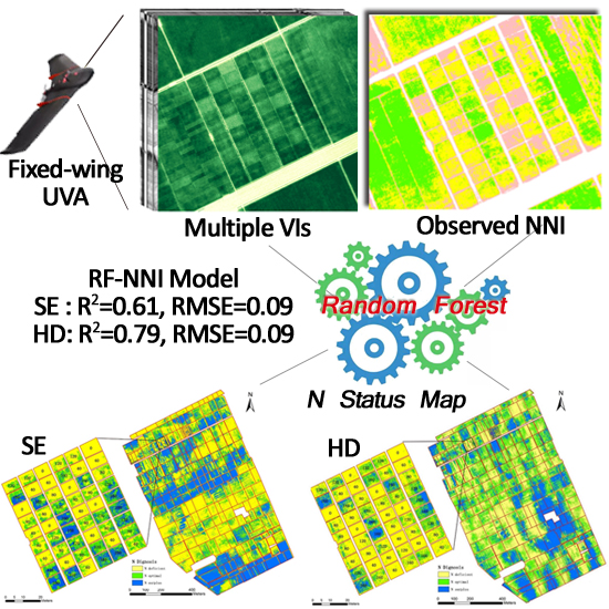
Improving Unmanned Aerial Vehicle Remote Sensing-Based Rice Nitrogen Nutrition Index Prediction with Machine Learning

1
International Center for Agro-Informatics and Sustainable Development (ICASD), College of Resources and Environmental Sciences, China Agricultural University, Beijing 100193, China
2
Precision Agriculture Center, Department of Soil, Water and Climate, University of Minnesota, St. Paul, MN 55108, USA
3
Center for Precision Agriculture, Norwegian Institute of Bioeconomy Research (NIBIO), Nylinna 226, 2849 Kapp, Norway
*
Author to whom correspondence should be addressed.
Remote Sens. 2020, 12(2), 215; https://doi.org/10.3390/rs12020215
Submission received: 13 December 2019 / Revised: 4 January 2020 / Accepted: 6 January 2020 / Published: 8 January 2020
(This article belongs to the Special Issue Remote Sensing for Precision Nitrogen Management)

Abstract

:
Optimizing nitrogen (N) management in rice is crucial for China’s food security and sustainable agricultural development. Nondestructive crop growth monitoring based on remote sensing technologies can accurately assess crop N status, which may be used to guide the in-season site-specific N recommendations. The fixed-wing unmanned aerial vehicle (UAV)-based remote sensing is a low-cost, easy-to-operate technology for collecting spectral reflectance imagery, an important data source for precision N management. The relationships between many vegetation indices (VIs) derived from spectral reflectance data and crop parameters are known to be nonlinear. As a result, nonlinear machine learning methods have the potential to improve the estimation accuracy. The objective of this study was to evaluate five different approaches for estimating rice (Oryza sativa L.) aboveground biomass (AGB), plant N uptake (PNU), and N nutrition index (NNI) at stem elongation (SE) and heading (HD) stages in Northeast China: (1) single VI (SVI); (2) stepwise multiple linear regression (SMLR); (3) random forest (RF); (4) support vector machine (SVM); and (5) artificial neural networks (ANN) regression. The results indicated that machine learning methods improved the NNI estimation compared to VI-SLR and SMLR methods. The RF algorithm performed the best for estimating NNI (R2 = 0.94 (SE) and 0.96 (HD) for calibration and 0.61 (SE) and 0.79 (HD) for validation). The root mean square errors (RMSEs) were 0.09, and the relative errors were <10% in all the models. It is concluded that the RF machine learning regression can significantly improve the estimation of rice N status using UAV remote sensing. The application machine learning methods offers a new opportunity to better use remote sensing data for monitoring crop growth conditions and guiding precision crop management. More studies are needed to further improve these machine learning-based models by combining both remote sensing data and other related soil, weather, and management information for applications in precision N and crop management.

Graphical Abstract

1. Introduction

Rice (Oryza sativa L.) is one of the most important crops in the world, consumed by more than 60% of China’s population as a staple food. Rice production in China is a major consumer of nitrogen (N) fertilizers, but the N use efficiency (NUE) is less than 30% [1]. Uniform fertilizer application across the fields according to experience or regional guidelines is the common practice and can lead to over-application of N at low yielding areas. The over-application of N fertilizers can result in enhanced reactive N losses to the environment, affecting human health, ecosystem services, biodiversity, climate change, and sustainability [1,2]. Precision N management (PNM) has the potential to effectively improve NUE, reduce soil and groundwater pollution, and increase farmers’ income [2]. Efficient tools for rapid and in-season diagnosis of rice N status over large areas are essential for the practical implementation of the PNM strategies.
When N fertilizers are applied in the fields, they need to be converted to plant available forms (nitrate (NO3) or ammonium (NH4+)) before they can be used by plants. The time they take for these conversions depends on the fertilizer type, soil temperature, soil moisture, soil pH, and soil aeration, etc. [3]. In rice production, N fertilizers are recommended to be applied in several splits to improve NUE, including application before planting or transplanting (called basal N fertilizer), at tillering stage (called tiller N fertilizer), at panicle initiation or stem elongation stage (called panicle N fertilizer), and at heading stage (called grain N fertilizer). It is important to diagnose rice N status during the growing season at different key N application stages, so topdressing N rates can be adjusted to better meet crop N needs. N nutrition index (NNI) is a reliable N status indicator and is defined as the ratio of plant N concentration (PNC) over critical N concentration (Nc), which is the minimum PNC that will achieve maximum aboveground biomass (AGB) production [4,5,6]. NNI > 1 indicates surplus N supply, while NNI < 1 indicates N deficiency, and NNI around 1 represents optimal N nutritional status [6]. However, NNI determination requires destructive sampling and chemical analysis, which limits its application in PNM. Therefore, the interests in technologies allowing nondestructive estimation of NNI over large areas are increasing.
Proximal and remote sensing technologies are commonly used for estimating crop N status nondestructively and at low cost [7,8,9,10,11]. A number of studies have used proximal canopy sensors to estimate NNI of various crops [12,13,14,15,16,17]. However, the usage of proximal sensors is not efficient for large production fields and mounting the sensors on the ground vehicles is not suitable for rice production. Satellite remote sensing has also been used for monitoring crop growth and N status in large areas. The FORMOSAT-2 satellite images were used to estimate rice NNI and diagnose N status and the results indicated that a practical approach was to use the satellite images to estimate rice AGB and plant N uptake (PNU), which were then used to calculate Nc and NNI (R2 = 0.52) [2]. The potential of using FORMOSAT-2, RapidEye, and WorldView-2 satellite data to estimate rice NNI were also evaluated and the results indicated that WorldView-2 satellite data performed the best [18]. However, in rice production areas, complete overcast weather conditions are very common, and it is very challenging to obtain satellite image data at the growth stages needed for guiding in-season topdressing N recommendations.
In recent years, unmanned aerial vehicle (UAV)-based remote sensing has developed rapidly, due to its low cost, ease of operation, and wide field of view [19,20]. The advances in data processing software have followed, allowing for automated development of image products [21]. A number of studies have used UAV remote sensing for crop N status diagnosis in various crops [22,23,24,25,26,27]. Most of these studies focused on identifying the optimum vegetation index (VI) and used linear regression method to estimate NNI or other N status indicators. The research should advance towards including more significant VIs and using nonlinear methods to improve the N status diagnosis with UAV remote sensing.
Over the past decade, machine learning (ML) methods have been widely adopted in complex and data-intensive areas such as medicine, astronomy, biology, and precision agriculture, due to their capability to discover information hidden in the data [28]. One of the main advantages of ML is that they are capable of solving significant nonlinear problems using datasets from multiple sources [29]. Agricultural remote sensing inversion is a typical nonlinear problem, and ML has been applied to solve it with satisfactory results [30,31]. For example, Han et al. used UAV remote sensing data and ML to estimate maize (Zea mays L.) biomass (R2 = 0.70) [32]. Ali et al. developed a model for the estimation of grassland biomass by using adaptive neuro-fuzzy inference system and multi-temporal remote sensing (R2 = 0.85) [33]. Pantazi et al. developed an artificial neural network (ANN)-based wheat yield prediction model using normalized difference VI (NDVI) derived from satellite imagery and eight soil parameters [34]. Liu et al. estimated wheat leaf N content using a multilayer perceptron neural network model and hyperspectral image data [35]. Zheng et al. compared different ML methods for estimating winter wheat leaf N content using UAV multispectral images and found that the fast processing random forest (RF) algorithm performed the best among the tested methods (R2 = 0.79, RMSE = 0.33) [36].
The literature of using ML on the UAV-borne reflectance data for rice crop N status is limited. Therefore, the objective of this study was to evaluate five different approaches for estimating rice aboveground biomass (AGB), plant N uptake (PNU), and N nutrition index (NNI) at stem elongation (SE) and heading (HD) stages in Northeast China: (1) single VI (SVI); (2) stepwise multiple linear regression (SMLR); (3) random forest (RF); (4) support vector machine (SVM); and (5) artificial neural networks (ANN) regression. Our hypothesis is that the machine learning methods can analyze both linear and nonlinear relationships between a dependent variable and multiple independent variables and can improve the prediction of rice N status indicators using multiple VIs than methods using single VI or multiple linear regression method using multiple VIs. This paper is organized in the following sections: Section 1 provides an introduction of the background and objective of this research. Section 2 describes the field experiments, data collection and analysis methods. Section 3 presents the results, and Section 4 discusses the results. Section 5 concludes this research.

2. Materials and Methods
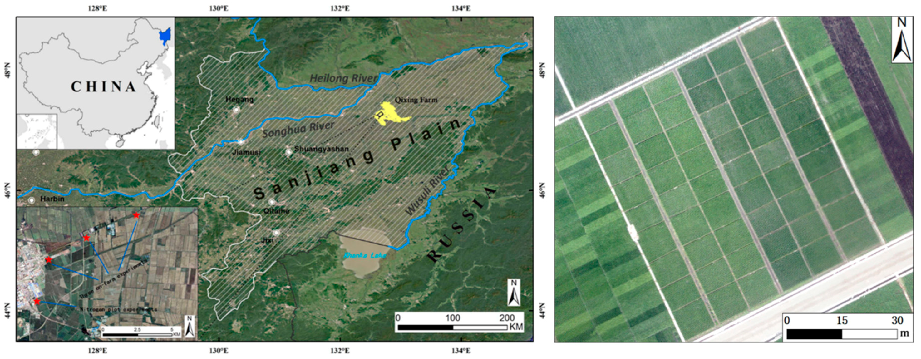
2.1. Study Site

The study site is located at the Jiangsanjiang Experiment Station of the China Agricultural University (47.2°N, 132.6°E) in the Sanjiang Plain of Heilongjiang Province, Northeast China (Figure 1). Sanjiang Plain belongs to a typical cool-temperate sub-humid continental monsoon climate zone. Japonica rice is the main planting crop in this cold region. The average sunshine hours are about 2300–2600 per year, the frost-free period is only about 110–135 days per year. The mean annual temperature is about 2 °C, and the average daily temperature is 19.9 °C during the growing season. The average rainfall is 500–600 mm per year, about 72% of which occurs between June and September [4]. The primary soil type in the Sanjiang Plain is Albic soil, classified as Mollic Planosols in the FAO-UNESCO system and Typical Argialbolls in Soil Taxonomy [37].

2.2. Experimental Setup

Ten plot experiments were conducted in 2017 and 2018 involving two Japonica rice cultivars Longjing 31 (with 11 leaves) and Longjing 21 (with 12 leaves), five N rates (0, 40, 80, 120, and 160 kg N ha−1), two different planting densities (27 and 33 hills m−2). All of the experiments adopted the randomized complete block design with three replicates (Figure 1). The size of each plot was 7 × 9 m and did not change during the study period. The N fertilizer was applied with three splits in the N rate experiments: 40% as basal application before transplanting, 30% at the tillering stage, and 30% at the stem elongation (SE) stage. Phosphorus and potassium fertilizers were applied uniformly across the plot experiments at the rates of 50 kg P2O5 ha−1 and 105 kg K2O ha−1, respectively. Phosphorus was applied in a single rate before transplanting and potassium was applied in two equal splits before transplanting and at the SE growth stage.
In addition to the plot experiments, three on-farm experiments were conducted in cooperation with three selected farmers of Qixing Farm in 2017 and 2018 in order to compare different precision rice management systems (Figure 1). The soil organic matter (OM) content was 30.2, 37.5, and 43.2 g kg−1 for Fields 1, 2, and 3, respectively. Treatments in each experiment included (1) Farmer’s Practice (FP); (2) Regional Optimal Management (ROM); (3) Precision Rice Management 1 (PRM1) with remote sensing-based N recommendation at stem elongation stage; (4) PRM2; and (5) PRM3. PRM2 and 3 used two different rates of controlled-release fertilizer as basal fertilizer. The plot size for each treatment varied from 20 × 8 m to 30 × 10 m, depending on the farmer’s field situation. The rice cultivar was Longjing 31 (an 11 leaf cultivar), and each treatment was performed in triplicate. The details of planting density and N application rates are given in Table 1.
These plot and on-farm experiments were conducted for other objectives, but this study took advantage of the variable N status in these experiments to evaluate different UAV remote sensing-based N status estimation methods.

2.3. Field Data Collection and NNI Parametrization

After spectral data collection at the SE and heading (HD) growth stages, three hills of rice plants were randomly selected according to the average tillering numbers in each plot and removed with roots. They were washed with clear water, and the roots were removed with scissors. The cleaned samples were separated into leaves, stems, and panicles (at heading), put into the oven under 105 °C for 30 min to deactivate the enzymes, and then dried to a constant weight at about 80 °C to determine dry AGB. N concentrations for leaves, stems, and panicles were determined using the standard Kjeldahl method [38]. PNC was determined based on the weighted average of the N content of all rice organs. The PNU was determined by multiplying PNC with AGB.
The critical N dilution curve of rice in Northeast China developed by Huang et al. [8] shown in Equation (1) was used in this research for AGB larger than 1 t ha−1:
Nc = 27.7W − 0.34,
where Nc is the critical N concentration (%) in the AGB, and W is the shoot dry weight expressed in t ha−1. For AGB less than 1 t ha−1, the Nc was set to a concentration of 2.77%.
The NNI was calculated using Equation (2)
NNI = Na/Nc,
where Na is the measured N concentration.
The NNI was also alternatively calculated using PNU, as given in Equation (3)
NNI = PNU/(Nc × AGB),
where PNU is plant N uptake (kg ha−1), and AGB is the aboveground biomass in t ha−1.

2.4. UAV Image Acquisition and Preprocessing

This study utilized the eBee SQ fixed-wing UAV system (SenseFly, Cheseaux-sur-Lausanne, Switzerland) with Parrot Sequoia camera onboard. This camera includes a four-band multispectral camera (1.2 MP, 1280 × 960 pixels) with a green band (550 + 20 nm), red band (660 + 20 nm), Red edge band (735 + 5 nm), the near-infrared band (790 + 20 nm) and Red Green Blue (RGB) camera (16 MP, 4608 × 3456 pixels). The unit is equipped with the upwards-oriented irradiance sensor for automated control of the integration time on the detectors. The camera system was referenced for the current downwelling radiation before each flight mission using a white Spectralon® panel (Labsphere, Inc., North Sutton, NH, USA). The UAV missions were conducted between 10:00 and 14:00, under windless and clear-sky conditions.
The UAV mission control and image acquisition were performed by the flight control software eMotion Ag 3.5.0 (SenseFly, Cheseaux-sur-Lausanne, Switzerland). The flight altitude was 106 m, the ground sampling distance was about 0.1 m per pixel and the images were taken with the forward overlap and the side overlap of 85% and 75%, respectively [39]. After the data acquisition, the geotagged images were mosaicked using Pix4Dmapper Ag software (Pix4D SA, Prilly, Switzerland) to obtain the spectral reflectance image of the entire scene, covering the whole experimental area. The mosaic was later orthorectified in ENVI 5.1 software (ENVI, Harris Geospatial Solutions, Inc., Boulder, Colorado, USA), using the ground control points referenced by a survey-grade GNSS receiver (CHCNAV, LT500, Shanghai, China) [39]. A total of four UAV reflectance orthoimages were obtained at the SE and HD growth stages in 2017 and 2018. The plot boundaries were digitized and used as regions of interest to select and average image pixels at a given sampling point in order to relate them to the groundtruth data.

2.5. Data Analysis

In this study, the reflectance data from the four spectral bands were used to calculate 72 VIs (Table A1) and both raw reflectance data of the three wavebands and VIs were used in the analyses. The calculated VIs were ranked by R2 for their relationships with AGB, PNU, and NNI and the top performing indices were further investigated.
The data collected in 2017 and 2018 were pulled together and then randomly divided into training dataset (70%) and test dataset (30%). A total of 381 observations were obtained in 2017 and 2018, 266 of which were used as training dataset and 115 as test dataset (Table 2). Among the analyzed crop properties, the AGB was the most variable parameter, with coefficient of variation (CV) being 37.54% for training and 42.37% for the test dataset, followed by PNU (CV% of 34.31% and 39.59%). PNC and NNI had similar variability, with CV of 6.03% and 16.42% in the training dataset and 15.47% and 17.86% in the test dataset, respectively. NNI ranged from 0.57 to 1.28 in the training dataset, and 0.58 to 1.21 in the test dataset. The data range of all training datasets encompassed the test dataset range, which ensured that the test data would not exceed the scope of the trained models. The training dataset was used to establish the simple regression models using linear, quadratic, power, exponential, and logarithmic functions or SMLR models between the VIs and AGB, PNU, and NNI. Established models were evaluated using the test dataset. The coefficient of determination (R2), root mean square error (RMSE), and relative error (RE) were used to assess the models. The higher the R2 and the lower the RMSE and RE, the higher was the precision and accuracy of the model for predicting the N status indicators. The scikit-learn [40,41], a Python machine learning library, was used in this study to establish models for estimation of AGB, PNU, and NNI using three conventional ML methods: RF, SVM, and ANN regressions. Tenfold cross-verification and grid search were used to find the optimal parameters during model development. The test dataset and R2, RMSE, RE were used to evaluate the accuracy of the models.

3. Results

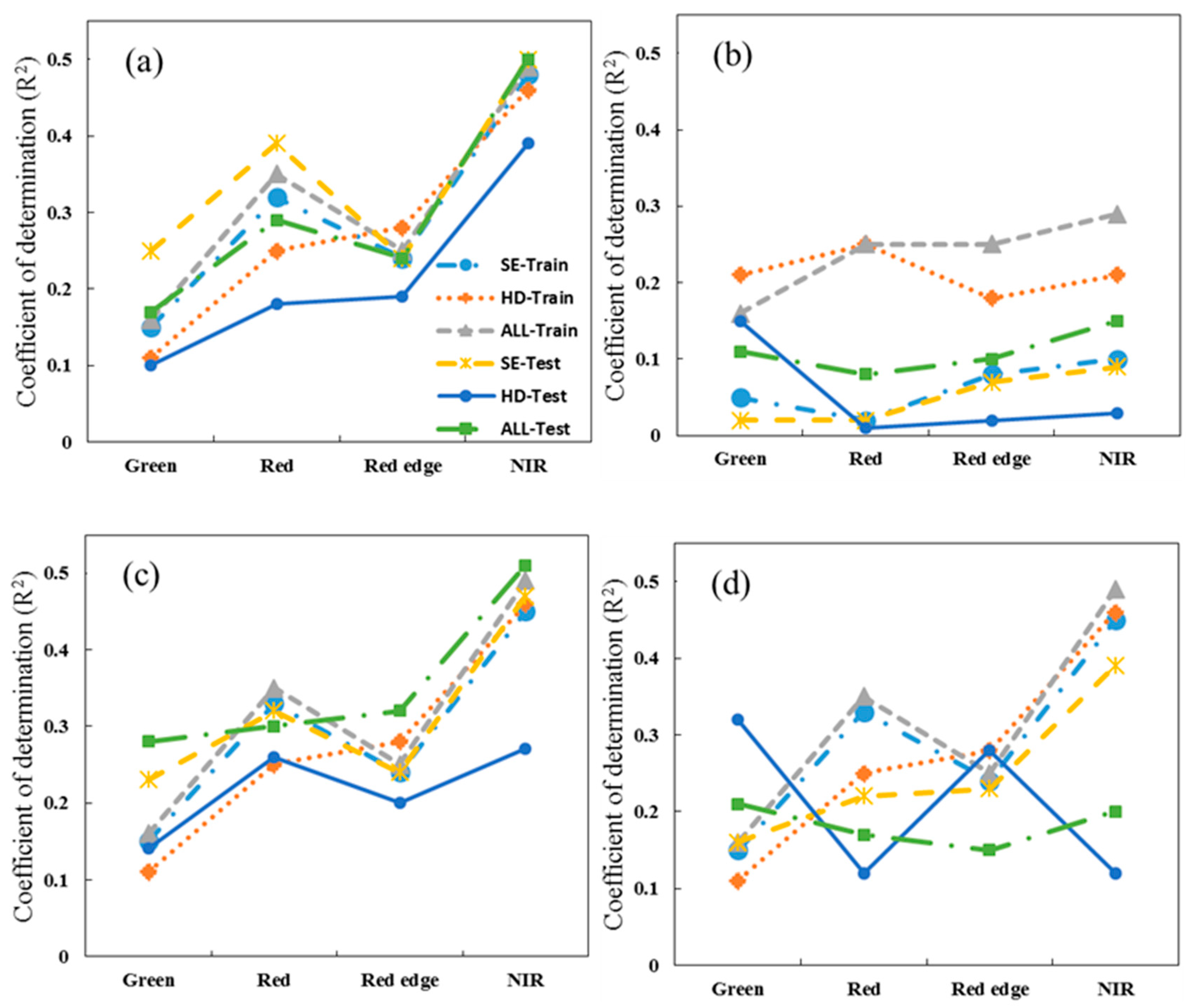
3.1. Single Spectral Band Analysis

The coefficient of determination for the relationships between the reflectance of each of the four wavebands and rice N status indicators at different growth stages are shown in Figure 2 for both training and testing datasets. The NIR band consistently had the highest R2 for AGB and PNU, while for PNC and NNI, the sensitivity of different wavebands changed with growth stages. In general, the relationships between reflectance of different wavebands and PNC were weaker than other N status indicators.

3.2. Vegetation Index Analysis

The three top performing VIs for estimating rice N status indicators based on the training dataset are given in Table 3. At best, a single VI could explain 65%, 65%, and 74% of AGB variation at the SE, HD, and across growth stages, respectively. The corresponding R2 was 0.61, 0.69, and 0.73 for PNU at SE, HD, and across stages, respectively. For NNI, 43%, 63%, and 39% of the variabilities were explained by the best VI at SE, HD, and across growth stages, respectively. All these relationships were significant at p < 0.01.
The VIs with the highest R2 were selected to establish the regression models for prediction of AGB, PNU, and NNI, which were validated using the test dataset and the results are shown in Figure 3. The models performed worse for AGB and PNU at SE and HD stages compared with calibration models, but slightly better across growth stages. For NNI, the models performed better with the test dataset. The indirect estimation of NNI performed slightly better than the direct approach at SE and HD stages, but somewhat worse across growth stages (Figure 4).

3.3. Stepwise Multiple Linear Regression (SMLR) Analysis

The SMLR analysis results indicated that the models could explain 69%, 62%, and 68% of AGB variation at SE, HD, and across stages using 2–4 VIs, respectively (Table 4). Similar results were obtained for PNU. These models explained 54%, 75%, and 40% of the NNI variability at the SE, HD, and across stages, respectively. These models performed better than models based on single VI in terms of R2, RMSE, and RE.
The test results given in Table 5 indicate that the SMLR performed better at estimating AGB and NNI than models using single VI, while for PNU estimation, the two modeling methods performed similarly. Moreover, the results of indirect prediction of NNI were similar to the results of direct prediction.

3.4. Performance of Machine Learning Models

For estimating AGB and PNU, the RF and ANN models consistently performed better than the SVM models, while for NNI, the RF model consistently performed the best at different growth stages, based on the calibration dataset (Table 6). The validation results indicated that the RF models performed consistently the best among the tested methods, including the indirect estimation of NNI (Table 7). Some models, especially those based on the ANN method, did not validate well with the test dataset, indicating the problem of overfitting.

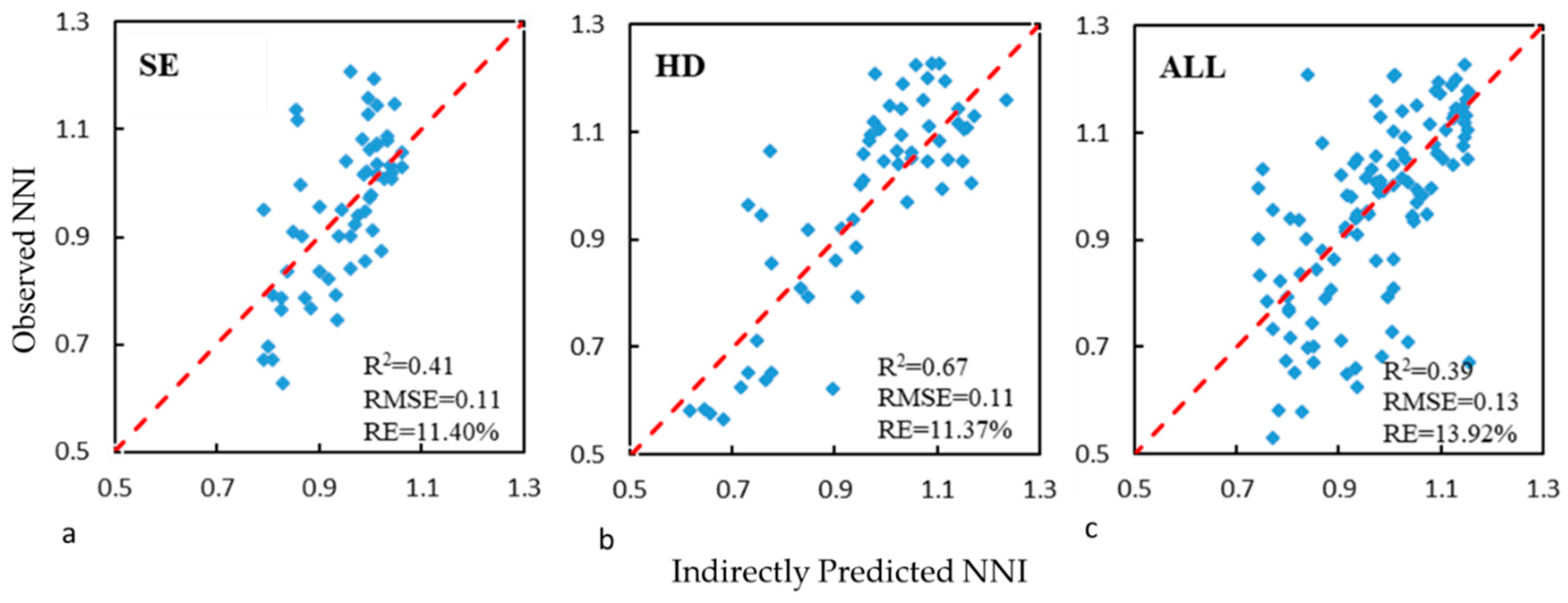
3.5. Random Forest Models Based on Selected Vegetation Indices

For practical applications, the RF models were optimized by removing VIs not important for the performance of the model. This resulted in simpler models, yet with comparable performance to the models based on all the tested VIs (Table 8). Models established at the SE stage, although outperforming the models based on single VI or SMLR models, performed worse in comparison with the models at the HD stage and across stages. The indirect NNI estimation approach gave worse results than the direct approach, which was similar to the results obtained with SMLR analysis.
Depending on the analyzed subset, from 17 to 23 VIs were selected by the RF models at different growth stages and the top five VIs are listed in Table 9. The relative importance of different VIs changed with growth stages or dependent variables. Green Optimized Soil Adjusted Vegetation Index (GOSAVI) was consistently selected among the top five indices at SE, HD, or across growth stages for both AGB and NNI prediction, and at SE and HD stages for PNU prediction. Normalized near-infrared (NNIR) and red edge difference vegetation index (REDVI) were among the top five indices for AGB and PNU at the SE stage, and for NNI at both SE and HD stages.

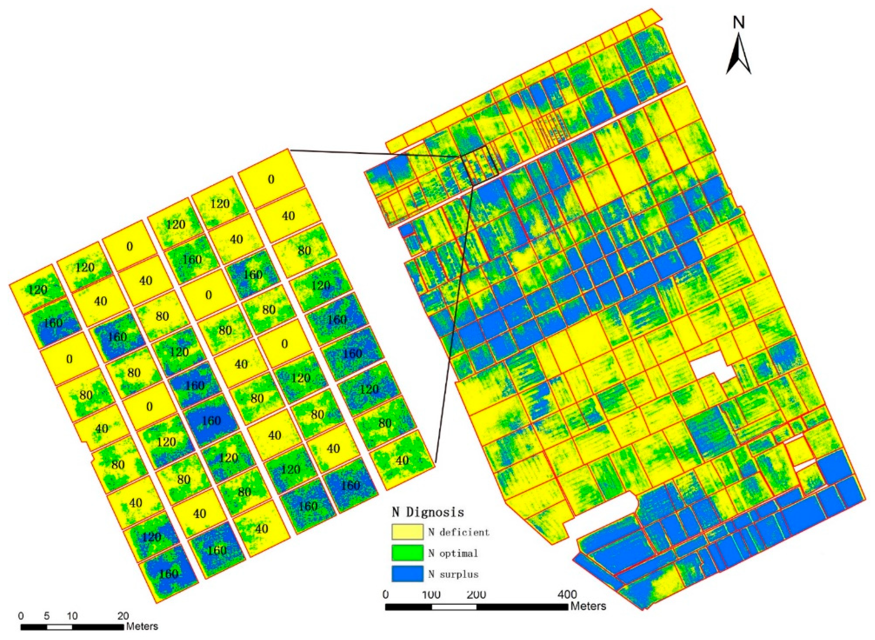
3.6. Nitrogen Status Diagnosis at the Farm Scale

The N status diagnosis maps for the study area were created based on the predicted NNI using the fixed wing UAV remote sensing images and the RF models at the SE (Figure 5) and HD (Figure 6) stages in 2017. At the SE stage, the majority fields had optimal or surplus N status, with less N deficient areas (Figure 3). At the HD stage, the majority fields had deficient or surplus N status, with less areas having optimal N status (Figure 4). For the N plot experiments, most of the plots receiving less than 120 kg N ha−1 were classified as N deficient, while most plots receiving 160 kg N ha−1 were classified as surplus N, whereas parts of these plots were also categorized as optimal N and parts of plots receiving 120 kg N ha−1 were also classified as N surplus.

4. Discussion

4.1. Estimating Rice N Status Indicators Using Single Vegetation Index

Using UAV-based remote sensing for in-season crop N status diagnosis and guiding variable rate N application is very attractive. The reflectance of single spectral bands can be used to estimate crop N status, as indicated by the results of this study. However, this approach only uses the reflectance of only one spectral band. A common approach to use reflectance information from more than one spectral band is to develop VIs, which are mathematical combinations of reflectance from two or more spectral bands. VIs are expected to perform better than single spectral wavebands. Many different factors may influence the performance of VIs, including soil and water backgrounds, weeds, cover crops in the interrow, the types of plants, and the growth stages of crops, etc. [42]. Growth stage can have a strong influence on the sensitivity and performance of different wavelengths and VIs for estimating crop parameters [43,44]. For rice, soil and water background can have a strong influence on canopy reflectance at early growing season before rice canopy closure (e.g., tillering stage or SE stage). At later growth stages with canopy closure (e.g., HD stage), some VIs like normalized difference vegetation index (NDVI) can become saturated [44]. In addition, the emergence of panicles makes the canopy reflectance more complicated, increasing the reflectance in visible spectral region but decreasing reflectance in the NIR region [45]. As a result, many different VIs have been developed for different applications [42]. It is necessary to evaluate the published VIs and identify the best performing VIs for a particular application (e.g., estimation of rice N status indicators).
The results of this study indicated that GOSAVI, Nonlinear Index (NLI), and Modified Green Soil Adjusted Vegetation Index (MGSAVI) performed best, explaining 65%, 65%, and 74% of rice AGB variability at SE, HD, and across growth stages, respectively. The GOSAVI explained 61%, 69%, and 73% of PNU variability at the SE, HD, and across growth stages, respectively. However, at best 63% of the NNI variability could be explained by Green Normalized Difference Vegetation Index (GNDVI) at the HD stage, but only 43% and 39% of NNI variability could be explained at the SE and across stages. The results of Cao et al. using active canopy sensor Crop Circle ACS-470 indicated that 54%–79%, 59%–83%, and 59%–77% of rice AGB, PNU, and NNI variabilities could be explained by the best performing VIs, respectively [46]. This study gave similar results for AGB and PNU, however the NNI estimations at SE and across growth stages were worse than the results obtained by Cao et al. [46]. This may be due to the fact that the UAV image sampling included the entire areas of the plots. The soil and water background may have more influence on the reflectance when compared with handheld canopy sensor in the study of Cao et al. [46]. As a result, using UAV remote sensing and VI-based approach could not achieve acceptable NNI estimation at the SE stage before canopy closure. In a similar research with winter wheat across smallholder farmer fields, Chen et al. explained 72%, 64%, and 46% variation in winter wheat (Triticum aestivum L.) AGB, PNU, and NNI at the SE stage using single VI-based approach with eBee SQ UAV remote sensing [39]. Their results were comparable to our results, with AGB and PNU being better predicted than NNI.

4.2. The Performance of Different Machine Learning Modeling Methods

In addition to single VI, SMLR and three different ML algorithms were applied to predict rice N status indicators in this study. The SMLR model performed significantly better than models based on single VI. Our results are consistent with the results of previous studies with winter wheat [47]. SMLR models use more VIs with spectral information related to the variables of interest and are flexible and easy to perform [48,49,50,51].
The SMLR models can only model linear combination of predictors [52], while the ML models can also model nonlinear relationships. The RF regression algorithm is an ensemble-learning algorithm that combines a broad set of regression trees. A regression tree represents a set of conditions or restrictions that are hierarchically organized and successively applied from a root to a leaf of the tree [53,54,55]. The SVM algorithm is based on statistical learning theory and can be regarded as the same type of network, can also be used for both classification and regression problems [56]. ANN regression is based on the gradient learning method. It is a nonparametric nonlinear model that uses neural network spreading between layers and simulates human brain receivers and information processing [57,58]. All three ML models performed better than models based on single VI. The three ML models all achieved better results than SMLR models in calibration, but in the validation analysis, only the RF models performed consistently better than SMLR. The possible reason for such results is that ML modeling often results in an over-fitting phenomenon, and the robustness and generalization ability of RF are stronger than the other ML methods [31,36,58,59,60].
The results of NNI indirect estimation approach were generally worse than the direct estimation approach. This is possibly due to the estimation of AGB and PNU in the indirect estimation approach that led to the accumulation of errors.
In summary, the results of this study indicated that the RF algorithm could be used to predict NNI directly at different growth stages. It performed better than other evaluated approaches. The NNIR and REDVI indices were the most important predictors at the SE stage, GNDVI and NNIR were most important at the HD stage, while green chlorophyll index (CIg) and GOSAVI were the most important predictors across growth stages. The relative importance of different VIs varied with growth stages and N status indicators. NNIR, REDVI, and other VIs containing red edge and near-infrared bands were more important for NNI estimation. Some of the VIs were significantly correlated. When the model needs to select input parameters, if the correlation between two VIs is very high, the RF model tends to select only one VI and abandons the other. Many of the VIs with small weights were selected in the models, because these algorithms need to use more dimensions to explain the variation of the data.

4.3. Challenges and Future Research Needs

In this study, multispectral data and VIs were obtained using fixed-wing UAV remote sensing, and the rice NNI distribution maps at different growth stages were created based on RF model prediction. The NNI map at the SE stage can be used to guide farmers to apply N fertilizers at the variable rates. The use of fixed-wing UAV remote sensing can effectively overcome the limitations of satellite remote sensing and proximal crop canopy sensing, and provide a reliable data source for diagnosis of the rice N nutritional status and in-season variable rate recommendation.
At present, most UAVs for remote sensing are powered with batteries, and the operation time is still quite short. For example, the eBee SQ system can only fly about 40 min, which limits the data acquisition ability of a single UAV operator. If UAVs adopt larger battery capacities and more effective battery charging in the future, effectively solving the problem of insufficient power, it will greatly increase the operational efficiency and the area monitored by a single unit. In addition, the field preparation for setting up ground control points, reflectance panels, and flight design is also very time consuming. The advances in technology have made it possible to achieve similar precision without the use of ground control points, to get rid of ground reflectance panels by using incident light sensors and greatly simplify flight design [61]. UAV remote sensing is also significantly affected by weather conditions, like winds, rain, or clouds [61,62]. Mounting active canopy sensors on UAV may provide a practical solution to such weather limitations [63].
In this study, UAV image-based rice crop reflectance was the single data source used in the ML models. This alone showed that nonlinear ML models improved NNI estimation compared to the simple VI-based methods. In addition to the commonly used red, green, blue, red edge, and near-infrared bands, other spectral regions should be studied for N status diagnosis, like shortwave infrared (SWIR)-based indices [45,64] or using hyperspectral cameras [62]. Studies found that a combination of multispectral and thermal images using relevance vector machines improved the estimation of plant chlorophyll concentration [65] and has the potential to simultaneously identify N and water stress. In the future, meteorological data, soil data, terrain attributes, and the information about crop management can be used together with remote sensing data to improve the performance of the ML models and NNI estimation [66].

5. Conclusions

In this study, eBee SQ UAV images were used to evaluate the VI, SMLR, and three ML algorithms (RF, SVM, and ANN) to estimate rice AGB, PNU, and NNI at the SE, HD, and across stages, and the NNI maps were created to diagnose N nutritional status of rice fields at the study site in Northeast China. The results indicated that ML methods could significantly improve the estimation of rice NNI compared to single VI and SMLR models, especially using an optimized RF algorithm, with 94% and 96% of the NNI variability being explained for the calibration dataset at the SE and HD stages, respectively, and 61% and 79% of NNI variability being explained for the test dataset at the SE and HD stages, respectively. The RMSE was 0.09, and RE was less than 10%. It is concluded that the RF modeling method can significantly improve the prediction of rice NNI using UAV remote sensing. The application machine learning methods offers a new opportunity to better use remote sensing data for monitoring crop growth conditions and guiding precision crop management. More studies are needed to further improve these machine learning-based models by combining both remote sensing data and other related soil, weather, and management information for applications in precision N and crop management.

Author Contributions

Y.M. and H.Z. conceptualized and designed the research. H.Z., T.W., Y.L., J.Z., W.S., and Z.F. conducted the field experiments and performed data collection. H.Z. analyzed the data and wrote the original manuscript. Y.M. and K.K. reviewed and revised the paper. The research was supervised by Y.M. and K.K. secured the research funding and managed the projects. All authors have read and agreed to the published version of the manuscript.

Funding

This research was funded by the Norwegian Ministry of Foreign Affairs (SINOGRAIN II, CHN-17/0019), the National Key Research and Development Program of China (2016YFD0200600, 2016YFD0200602), National Basic Research Program of China (2015CB150405), and the Internationalization Training and Promotion Project of Graduate Students in China Agricultural University.

Acknowledgments

The authors thank Guojun Li, Yankai Niu, and Guangming Zhao at Jansanjiang Bureau of Agriculture in Heilongjiang Province, Beijing Aoteng Yanshi Technology Co., Ltd., and Anhui Yigang Information Technology Co., Ltd. for their assistance during this research. We also would like to thank all of the farmers for their cooperation in this research.

Conflicts of Interest

The authors declare no conflict of interest.

Appendix A

Table A1. The vegetation indices evaluated in this study. G, R, RE, and NIR indicate green red, red edge, and near infrared band reflectance.
IndexFormulaReference
Green Ratio Vegetation Index (GRVI)NIR/G[67]
Green Difference Vegetation Index (GDVI)NIR − G[68]
Green Normalized Difference Vegetation Index (GNDVI)(NIR − G)/(NIR + G)[69]
Green Wide Dynamic Range Vegetation Index (GWDRVI)(a*NIR − G)/(a*NIR + G) (a = 0.12)[46]
Green Chlorophyll Index (CIg)NIR/G − 1[70]
Modified Green Simple Ratio (MSR_G)(NIR/G − 1)/SQRT(NIR/G + 1)[46]
Green Soil Adjusted Vegetation Index (GSAVI)1.5*[(NIR − G)/(NIR + G + 0.5)][71]
Modified Soil Adjusted Vegetation Index (MSAVI)0.5*[2*NIR + 1 − SQRT((2*NIR + 1)2 − 8*(NIR − G))][72]
Green Optimal Soil Adjusted Vegetation Index (GOSAVI)(1 + 0.16)(NIR − G)/(NIR + G + 0.16)[73]
Green Re-normalized Different Vegetation Index (GRDVI)(NIR − G)/SQRT(NIR + G)[46]
Normalized Green Index (NGI)G/(NIR + RE + G)[71]
Normalized Red Edge Index (NREI)RE/(NIR + RE + G)[46]
Normalized Red Index (NRI)R/(NIR + RE + R) [14]
Normalized NIR Index (NNIR)NIR/(NIR + RE + G)[71]
Modified Double Difference Index (MDD)(NIR − RE) − (RE − G)[14]
Modified Normalized Difference Index (MNDI)(NIR − RE)/(NIR − G)[46]
Modified Enhanced Vegetation Index (MEVI)2.5*(NIR − RE)/(NIR + 6*RE − 7.5*G + 1)[46]
Modified Normalized Difference Red Edge (MNDRE)[NIR − (RE − 2*G)]/[NIR + (RE − 2*G)][46]
Modified Chlorophyll Absorption In Reflectance Index1 (MCARI1)[(NIR − RE) − 0.2*(NIR − R)](NIR/RE)[46]
Modified Chlorophyll Absorption In Reflectance Index 2 (MCARI2) 1.5 [ 2.5 ( N I R R ) 1.3 ( N I R R E ) ] ( 2 N I R + 1 ) 2 ( 6 N I R 5 R ) 0.5 [14]
Normalized Difference Vegetation Index (NDVI)(NIR − R)/(NIR + R)[74]
Ratio Vegetation Index( RVI)NIR/R[75]
Difference Vegetation Index (DVI)NIR − R[68]
Renormalized Difference Vegetation Index (RDVI) (NIR − R)/SQRT(NIR + R)[76]
Wide Dynamic Range Vegetation Index (WDRVI)(a*NIR − R)/(a*NIR + R) (a = 0.12)[77]
Soil-Adjusted Vegetation Index (SAVI)1.5*(NIR − R)/(NIR + R + 0.5)[78]
Optimized SAVI (OSAVI)(1 + 0.16)*(NIR − R)/(NIR + R + 0.16)[73]
Modified Soil-adjusted Vegetation Index (MSAVI)0.5*[2*NIR + 1 − SQRT((2*NIR + 1)2 − 8*(NIR − R))][72]
Transformed Normalized Vegetation Index (TNDVI)SQRT((NIR − R)/(NIR + R) + 0.5)[79]
Modified Simple Ratio (MSR)(NIR/R − 1)/SQRT(NIR/R + 1)[80]
Optimal Vegetation Index (VIopt)1.45*((NIR2 + 1)/(R + 0.45))[81]
MERIS Terrestrial Chlorophyll Index (MTCI)(NIR − RE)/(RE − R)[82]
Nonlinear Index (NLI)(NIR2 − R)/(NIR2 + R)[83]
Modified Nonlinear Index (MNLI)1.5*(NIR2 − R)/(NIR2 + R + 0.5)[84]
NDVI*RVI(NIR2 − R)/(NIR + R2)[84]
SAVI*SR(NIR2 − R)/[(NIR + R + 0.5)*R][84]
Normalized Difference Red Edge (NDRE)(NIR − RE)/(NIR + RE) [85]
Red Edge Ratio Vegetation Index (RERVI)NIR/RE[86]
Red Edge Difference Vegetation Index (REDVI)NIR − RE[46]
Red Edge Re-normalized Different Vegetation Index (RERDVI)(NIR − RE)/SQRT(NIR + RE)[46]
Red Edge Wide Dynamic Range Vegetation Index (REWDRVI)(a*NIR − RE)/(a*NIR + RE) (a = 0.12)[46]
Red Edge Soil Adjusted Vegetation Index (RESAVI)1.5*[(NIR − RE)/(NIR + RE + 0.5)][46]
Red Edge Optimal Soil Adjusted Vegetation Index (REOSAVI)(1 + 0.16)(NIR − RE)/(NIR + RE + 0.16)[46]
Modified Red Edge Soil Adjusted Vegetation Index (MRESAVI)0.5*[2*NIR + 1 − SQRT((2*NIR + 1)2 − 8*(NIR − RE))][46]
Optimized Red Edge Vegetation Index (REVIopt)100*(lnNIR − lnRE) [87]
Red Edge Chlorophyll Index (CIre)NIR/RE − 1[88]
Modified Red Edge Simple Ratio (MSR_RE)(NIR/RE − 1)/SQRT(NIR/RE + 1)[14]
Red Edge Normalized Difference Vegetation Index (RENDVI)(RE − R)/(RE + R)[89]
Red Edge Simple Ratio (RESR)RE/R[90]
Modified Red Edge Difference Vegetation Index (MREDVI)RE − R[46]
MERIS Terrestrial Chlorophyll Index (MTCI)(NIR − RE)/(RE − R)[82]
DATT Index (DATT)(NIR − RE)/(NIR − R) [91]
Normalized Near Infrared Index (NNIRI)NIR/(NIR + RE + R)[14]
Normalized Red Edge Index (NREI)RE/(NIR + RE + R)[14]
Normalized Red Index (NRI)R/(NIR + RE + R)[14]
Modified Double Difference Index (MDD)(NIR − RE) − (RE − R)[14]
Modified Red Edge Simple Ratio (MRESR)(NIR − R)/(RE − R)[14]
Modified Normalized Difference Index (MNDI)(NIR − RE)/(NIR + RE − 2R)[14]
Modified Enhanced Vegetation Index (MEVI)2.5*(NIR − R)/(NIR + 6*R − 7.5*RE + 1)[14]
Modified Normalized Difference Red Edge (MNDRE2)(NIR − RE + 2*R)/(NIR + RE − 2*R)[14]
Red Edge Transformed Vegetation Index (RETVI)0.5*[120*(NIR − R) − 200*(RE − R)][14]
Modified Chlorophyll Absorption In Reflectance Index 3 (MCARI3)[(NIR − RE) − 0.2*(NIR − R)](NIR/RE)[14]
Modified Chlorophyll Absorption In Reflectance Index 4 (MCARI4) 1.5 [ 2.5 ( N I R G ) 1.3 ( N I R R E ) ] ( 2 N I R + 1 ) 2 ( 6 N I R 5 G ) 0.5 [14]
Modified Transformed Chlorophyll Absorption In Reflectance Index (MTCARI)3*[(NIR − RE) − 0.2*(NIR − R)(NIR/RE)][14]
Modified Red Edge Transformed Vegetation Index (MRETVI)1.2*[1.2*(NIR − R) − 2.5*(RE − R)][14]
Modified Canopy Chlorophyll Content Index (MCCCI)NDRE/NDVI[92]
MCARI1/OSAVIMCARI1/OSAVI[14]
MCARI2/OSAVIMCARI2/OSAVI[14]
MTCARI/OSAVIMTCARI/OSAVI[14]
MCARI1/MRETVIMCARI1/MRETVI[14]
MTCARI/MRETVIMTCARI/MRETVI[14]

References

  1. Miao, Y.; Stewart, B.A.; Zhang, F. Long-term experiments for sustainable nutrient management in China. A review. Agron. Sustain. Dev. 2011, 31, 397–414. [Google Scholar] [CrossRef] [Green Version]
  2. Cao, Q.; Miao, Y.; Feng, G.; Gao, X.; Liu, B.; Liu, Y.; Li, F.; Khosla, R.; Mulla, D.J.; Zhang, F. Improving nitrogen use efficiency with minimal environmental risks using an active canopy sensor in a wheat-maize cropping system. Field Crop Res. 2017, 214, 365–372. [Google Scholar] [CrossRef]
  3. Havlin, J.L.; Tisdale, S.L.; Nelson, W.L.; Beaton, J.D. Soil Fertility and Fertilizers: An Introduction to Nutrient Management, 8th ed.; Pearson, Inc.: Upper Saddle River, NJ, USA, 2014; pp. 117–184. [Google Scholar]
  4. Huang, S.; Miao, Y.; Cao, Q.; Yao, Y.; Zhao, G.; Yu, W.; Shen, J.; Yu, K.; Bareth, G. A new critical nitrogen dilution curve for rice nitrogen status diagnosis in Northeast China. Pedosphere 2018, 28, 814–822. [Google Scholar] [CrossRef]
  5. Greenwood, D.; Gastal, F.; Lemaire, G.; Draycott, A.; Millard, P.; Neeteson, J. Growth rate and % N of field grown crops: Theory and experiments. Ann. Bot. 1991, 67, 181–190. [Google Scholar] [CrossRef]
  6. Lemaire, G.; Jeuffroy, M.; Gastal, F. Diagnosis tool for plant and crop N status in vegetative stage. Eur. J. Agron. 2008, 28, 614–624. [Google Scholar] [CrossRef]
  7. Inoue, Y.; Sakaiya, E.; Zhu, Y.; Takahashi, W. Diagnostic mapping of canopy nitrogen content in rice based on hyperspectral measurements. Remote Sens. Environ. 2012, 126, 210–221. [Google Scholar] [CrossRef]
  8. Filella, I.; Serrano, L.; Serra, J.; Penuelas, J. Evaluating wheat nitrogen status with canopy reflectance indices and discriminant analysis. Crop Sci. 1995, 35, 1400–1405. [Google Scholar] [CrossRef]
  9. Caturegli, L.; Corniglia, M.; Gaetani, M.; Grossi, N.; Magni, S.; Migliazzi, M.; Angelini, L.; Mazzoncini, M.; Silvestri, N.; Fontanelli, M.; et al. Unmanned aerial vehicle to estimate nitrogen status of turfgrasses. PLoS ONE 2016, 11, e158268. [Google Scholar] [CrossRef] [Green Version]
  10. Jay, S.; Maupas, F.; Bendoula, R.; Gorretta, N. Retrieving LAI, chlorophyll and nitrogen contents in sugar beet crops from multi-angular optical remote sensing: Comparison of vegetation indices and PROSAIL inversion for field phenotyping. Field Crop. Res. 2017, 210, 33–46. [Google Scholar] [CrossRef] [Green Version]
  11. Clevers, J.G.P.W.; Gitelson, A.A. Remote estimation of crop and grass chlorophyll and nitrogen content using red-edge bands on Sentinel-2 and -3. Int. J. Appl. Earth Obs. 2013, 23, 344–351. [Google Scholar] [CrossRef]
  12. Cao, Q.; Miao, Y.; Feng, G.; Gao, X.; Li, F.; Liu, B.; Yue, S.; Cheng, S.; Ustin, S.L.; Khosla, R. Active canopy sensing of winter wheat nitrogen status: An evaluation of two sensor systems. Comput. Electron. Agric. 2015, 112, 54–67. [Google Scholar] [CrossRef]
  13. Padilla, F.M.; Gallardo, M.; Pena-Fleitas, M.T.; Souza, R.D.; Thompson, R.B. Proximal optical sensors for nitrogen management of vegetable crops: A review. Sensors 2018, 18, 2083. [Google Scholar] [CrossRef] [Green Version]
  14. Lu, J.; Miao, Y.; Shi, W.; Li, J.; Yuan, F. Evaluating different approaches to non-destructive nitrogen status diagnosis of rice using portable RapidSCAN active canopy sensor. Sci. Rep. 2017, 7, 14073. [Google Scholar] [CrossRef]
  15. Morier, T.; Cambouris, A.N.; Chokmani, K. In-season nitrogen status assessment and yield estimation using hyperspectral vegetation indices in a potato crop. Agron. J. 2015, 107, 1295–1309. [Google Scholar] [CrossRef]
  16. Xia, T.; Miao, Y.; Wu, D.; Shao, H.; Khosla, R.; Mi, G. Active optical sensing of spring maize for in-season diagnosis of nitrogen status based on nitrogen nutrition index. Remote Sens. 2016, 8, 605. [Google Scholar] [CrossRef] [Green Version]
  17. Padilla, F.M.; Pena-Fleitas, M.T.; Gallardo, M.; Thompson, R.B. Evaluation of optical sensor measurements of canopy reflectance and of leaf flavonols and chlorophyll contents to assess crop nitrogen status of muskmelon. Eur. J. Agron. 2014, 58, 39–52. [Google Scholar] [CrossRef]
  18. Huang, S.; Miao, Y.; Yuan, F.; Gnyp, M.; Yao, Y.; Cao, Q.; Wang, H.; Lenz-Wiedemann, V.; Bareth, G. Potential of RapidEye and WorldView-2 satellite data for improving rice nitrogen status monitoring at different growth stages. Remote Sens. 2017, 9, 227. [Google Scholar] [CrossRef] [Green Version]
  19. Ham, Y.; Han, K.K.; Lin, J.J.; Golparvar-Fard, M. Visual monitoring of civil infrastructure systems via camera-equipped Unmanned Aerial Vehicles (UAVs): A review of related works. Vis. Eng. 2016, 4, 1. [Google Scholar] [CrossRef] [Green Version]
  20. Yang, G.; Liu, J.; Zhao, C.; Li, Z.; Huang, Y.; Yu, H.; Xu, B.; Yang, X.; Zhu, D.; Zhang, X. Unmanned aerial vehicle remote sensing for field-based crop phenotyping: Current status and perspectives. Front. Plant Sci. 2017, 8, 1111. [Google Scholar] [CrossRef]
  21. Yao, H.; Qin, R.; Chen, X. Unmanned aerial vehicle for remote sensing applications—A review. Remote Sens. 2019, 11, 1443. [Google Scholar] [CrossRef] [Green Version]
  22. Barbedo, J.G.A. A review on the use of unmanned aerial vehicles and imaging sensors for monitoring and assessing plant stresses. Drones 2019, 3, 40. [Google Scholar] [CrossRef] [Green Version]
  23. Deng, L.; Mao, Z.; Li, X.; Hu, Z.; Duan, F.; Yan, Y. UAV-based multispectral remote sensing for precision agriculture: A comparison between different cameras. ISPRS J. Photogramm. 2018, 146, 124–136. [Google Scholar] [CrossRef]
  24. Pajares, G. Overview and current status of remote sensing applications based on Unmanned Aerial Vehicles (UAVs). Photogramm. Eng. Remote Sens. 2015, 81, 281–330. [Google Scholar] [CrossRef] [Green Version]
  25. Severtson, D.; Callow, N.; Flower, K.; Neuhaus, A.; Olejnik, M.; Nansen, C. Unmanned aerial vehicle canopy reflectance data detects potassium deficiency and green peach aphid susceptibility in canola. Precis. Agric. 2016, 17, 659–677. [Google Scholar] [CrossRef] [Green Version]
  26. Vega, F.A.; Ramírez, F.C.; Saiz, M.P.; Rosúa, F.O. Multi-temporal imaging using an unmanned aerial vehicle for monitoring a sunflower crop. Biosyst. Eng. 2015, 132, 19–27. [Google Scholar] [CrossRef]
  27. Wang, H.; Mortensen, A.K.; Mao, P.; Boelt, B.; Gislum, R. Estimating the nitrogen nutrition index in grass seed crops using a UAV-mounted multispectral camera. Int. J. Remote Sens. 2019, 40, 2467–2482. [Google Scholar] [CrossRef]
  28. Qiu, J.; Wu, Q.; Ding, G.; Xu, Y.; Feng, S. A survey of machine learning for big data processing. EURASIP J. Adv. Signal Process. 2016, 2016, 67. [Google Scholar] [CrossRef] [Green Version]
  29. Chlingaryan, A.; Sukkarieh, S.; Whelan, B. Machine learning approaches for crop yield prediction and nitrogen status estimation in precision agriculture: A review. Comput. Electron. Agric. 2018, 151, 61–69. [Google Scholar] [CrossRef]
  30. Liakos, K.; Busato, P.; Moshou, D.; Pearson, S.; Bochtis, D. Machine learning in agriculture: A review. Sensors 2018, 18, 2674. [Google Scholar] [CrossRef] [Green Version]
  31. Ali, I.; Greifeneder, F.; Stamenkovic, J.; Neumann, M.; Notarnicola, C. Review of machine learning approaches for biomass and soil moisture retrievals from remote sensing data. Remote Sens. 2015, 7, 16398–16421. [Google Scholar] [CrossRef] [Green Version]
  32. Han, L.; Yang, G.; Dai, H.; Xu, B.; Yang, H.; Feng, H.; Li, Z.; Yang, X. Modeling maize above-ground biomass based on machine learning approaches using UAV remote-sensing data. Plant Methods 2019, 15, 10. [Google Scholar] [CrossRef] [PubMed] [Green Version]
  33. Ali, I.; Cawkwell, F.; Dwyer, E.; Green, S. Modeling managed grassland biomass estimation by using multitemporal remote sensing data—A machine learning approach. IEEE J. Sel. Top. Earth Obs. Remote Sens. 2017, 10, 3254–3264. [Google Scholar] [CrossRef]
  34. Pantazi, X.E.; Moshou, D.; Alexandridis, T.; Whetton, R.L.; Mouazen, A.M. Wheat yield prediction using machine learning and advanced sensing techniques. Comput. Electron. Agric. 2016, 121, 57–65. [Google Scholar] [CrossRef]
  35. Liu, H.; Zhu, H.; Wang, P. Quantitative modelling for leaf nitrogen content of winter wheat using UAV-based hyperspectral data. Int. J. Remote Sens. 2017, 38, 2117–2134. [Google Scholar] [CrossRef]
  36. Zheng, H.; Li, W.; Jiang, J.; Liu, Y.; Cheng, T.; Tian, Y.; Zhu, Y.; Cao, W.; Zhang, Y.; Yao, X. A comparative assessment of different modeling algorithms for estimating leaf nitrogen content in winter wheat using multispectral images from an unmanned aerial vehicle. Remote Sens. 2018, 10, 2026. [Google Scholar] [CrossRef] [Green Version]
  37. Xing, B.; Dudas, M.J.; Zhang, Z.; Xu, Q. Pedogenetic characteristics of albic soils in the three river plain, Heilongjiang Province. Acta Pedol. Sin. 1994, 31, 95–104. [Google Scholar]
  38. Lv, W.; Ge, Y.; Wu, J.; Chang, J. Study on the method for the determination of nitric nitrogen, ammoniacal nitrogen and total nitrogen in plant. Spectrosc. Spect. Anal. 2004, 24, 204–206. [Google Scholar]
  39. Chen, Z.; Miao, Y.; Lu, J.; Zhou, L.; Li, Y.; Zhang, H.; Lou, W.; Zhang, Z.; Kusnierek, K.; Liu, C. In-season diagnosis of winter wheat nitrogen status in smallholder farmer fields across a village using unmanned aerial vehicle-based remote sensing. Agronomy 2019, 9, 619. [Google Scholar] [CrossRef] [Green Version]
  40. Pedregosa, F.; Varoquaux, G.; Gramfort, A.; Michel, V.; Thirion, B.; Grisel, O.; Blondel, M.; Prettenhofer, P.; Weiss, R.; Dubourg, V. Scikit-learn: Machine learning in Python. J. Mach. Learn. Res. 2011, 12, 2825–2830. [Google Scholar]
  41. Abraham, A.; Pedregosa, F.; Eickenberg, M.; Gervais, P.; Mueller, A.; Kossaifi, J.; Gramfort, A.; Thirion, B.; Varoquaux, G. Machine learning for neuroimaging with scikit-learn. Front. Neuroinform. 2014, 8, 14. [Google Scholar] [CrossRef] [Green Version]
  42. Xue, J.; Su, B. Significant remote sensing vegetation indices: A review of developments and applications. J. Sens. 2017, 2017, 1353691. [Google Scholar] [CrossRef] [Green Version]
  43. Hatfield, J.L.; Prueger, J.H. Value of using different vegetative indices to quantify agricultural crop chateristics at different growth stages under varying management practices. Remote Sens. 2010, 2, 562–578. [Google Scholar] [CrossRef] [Green Version]
  44. Gnyp, M.L.; Miao, Y.; Yuan, F.; Ustin, S.L.; Yu, K.; Yao, Y.; Huang, S.; Bareth, G. Hyperspectral canopy sensing of paddy rice aboveground biomass at different growth stages. Field Crop Res. 2014, 155, 42–55. [Google Scholar] [CrossRef]
  45. Tang, Y.; Huang, J.; Wang, R. Change law of hyperspectral data in related with chlorophyll and carotenoid in rice at different developmental stages. Rice Sci. 2004, 11, 274–282. [Google Scholar]
  46. Cao, Q.; Miao, Y.; Wang, H.; Huang, S.; Cheng, S.; Khosla, R.; Jiang, R. Non-destructive estimation of rice plant nitrogen status with Crop Circle multispectral active canopy sensor. Field Crop. Res. 2013, 154, 133–144. [Google Scholar] [CrossRef]
  47. Jin, X.; Yang, G.; Xu, X.; Yang, H.; Feng, H.; Li, Z.; Shen, J.; Lan, Y.; Zhao, C. Combined multi-temporal optical and radar parameters for estimating LAI and biomass in winter wheat using HJ and RADARSAR-2 Data. Remote Sens. 2015, 7, 13251–13272. [Google Scholar] [CrossRef] [Green Version]
  48. Miao, Y.; Mulla, D.J.; Randall, G.W.; Vetsch, J.A.; Vintila, R. Combining chlorophyll meter readings and high spatial resolution remote sensing images for in-season site-specific nitrogen management of corn. Precis. Agric. 2009, 10, 45–62. [Google Scholar] [CrossRef]
  49. Faurtyot, T.; Baret, F. Vegetation water and dry matter contents estimated from top-of-the-atmosphere reflectance data: A simulation study. Remote Sens. Environ. 1997, 61, 34–45. [Google Scholar] [CrossRef]
  50. Chen, W.; Zhao, J.; Cao, C.; Tian, H. Shrub biomass estimation in semi-arid sandland ecosystem based on remote sensing technology. Glob. Ecol. Conserv. 2018, 16, e479. [Google Scholar] [CrossRef]
  51. Qin, H.; Wang, C.; Xi, X.; Tian, J.; Zhou, G. Estimation of coniferous forest aboveground biomass with aggregated airborne small-footprint LiDAR full-waveforms. Opt. Express 2017, 25, A851–A869. [Google Scholar] [CrossRef]
  52. Forkuor, G.; Hounkpatin, O.K.L.; Welp, G.; Thiel, M. High Resolution Mapping of Soil Properties Using Remote Sensing Variables in South-Western Burkina Faso: A comparison of machine learning and multiple linear regression models. PLoS ONE 2017, 12, e170478. [Google Scholar] [CrossRef] [PubMed]
  53. Breiman, L.; Friedman, J.; Olshen, R.; Stone, C. Classification and Regression Trees (The Wadsworth Statistics/Probability Series); Chapman and Hall/CRC: New York, NY, USA, 1984; pp. 1–358. [Google Scholar]
  54. Rodriguez-Galiano, V.; Mendes, M.P.; Garcia-Soldado, M.J.; Chica-Olmo, M.; Ribeiro, L. Predictive modeling of groundwater nitrate pollution using Random Forest and multisource variables related to intrinsic and specific vulnerability: A case study in an agricultural setting (Southern Spain). Sci. Total Environ. 2014, 476, 189–206. [Google Scholar] [CrossRef] [PubMed]
  55. Wang, L.; Zhou, X.; Zhu, X.; Dong, Z.; Guo, W. Estimation of biomass in wheat using random forest regression algorithm and remote sensing data. Crop J. 2016, 4, 212–219. [Google Scholar] [CrossRef] [Green Version]
  56. Durbha, S.S.; King, R.L.; Younan, N.H. Support vector machines regression for retrieval of leaf area index from multiangle imaging spectroradiometer. Remote Sens. Environ. 2007, 107, 348–361. [Google Scholar] [CrossRef]
  57. He, Q. Neural Network and its Application in IR. In Graduate School of Library and Information Science, University of Illinois at Urbana-Champaign; Spring: Champaign, IL, USA, 1999. [Google Scholar]
  58. Yuan, H.; Yang, G.; Li, C.; Wang, Y.; Liu, J.; Yu, H.; Feng, H.; Xu, B.; Zhao, X.; Yang, X. Retrieving soybean leaf area index from unmanned aerial vehicle hyperspectral remote sensing: Analysis of RF, ANN, and SVM Regression Models. Remote Sens. 2017, 9, 309. [Google Scholar] [CrossRef] [Green Version]
  59. Yao, X.; Huang, Y.; Shang, G.; Zhou, C.; Cheng, T.; Tian, Y.; Cao, W.; Zhu, Y. Evaluation of six algorithms to monitor wheat leaf nitrogen concentration. Remote Sens. 2015, 7, 14939–14966. [Google Scholar] [CrossRef] [Green Version]
  60. Yue, J.; Yang, G.; Li, C.; Li, Z.; Wang, Y.; Feng, H.; Xu, B. Estimation of winter wheat above-ground biomass using unmanned aerial vehicle-based snapshot hyperspectral sensor and crop height improved models. Remote Sens. 2017, 9, 708. [Google Scholar] [CrossRef] [Green Version]
  61. Tsouros, D.C.; Bibi, S.; Sarigiannidis, P.G. A review on UAV-based applications for precision agriculture. Information 2019, 10, 349. [Google Scholar] [CrossRef] [Green Version]
  62. Hunt, E.R., Jr.; Daughtry, C.S.T. What good are unmanned aircraft systems for agricultural remtoe sensing and precision agriculture? Int. J. Remote Sens. 2018, 39, 5345–5376. [Google Scholar] [CrossRef] [Green Version]
  63. Li, S.; Ding, X.; Kuang, Q.; Ata-Ul-Karim, S.T.; Cheng, T.; Liu, X.; Tian, Y.; Zhu, Y.; Cao, W.; Cao, Q. Potential of UAV-based active sensing for monitoring rice leaf nitrogen status. Front. Plant Sci. 2018, 9, 1834. [Google Scholar] [CrossRef] [Green Version]
  64. Herrmann, I.; Karnieli, A.; Bonfil, D.J.; Cohen, Y.; Alchanatis, V. SWIR-based spectral indices for assessing nitrogen content in potato fields. Int. J. Remote Sens. 2010, 31, 5127–5143. [Google Scholar] [CrossRef]
  65. Elarab, M.; Ticlavilca, A.M.; Torres-Rua, A.F.; Maslova, I.; McKee, M. Estimating chlorophyll with thermal and broadband multispectral high resolution imagery from an unmanned aerial system using relevance vector machines for precision agriculture. Int. J. Appl. Earth Observ. Geoinf. 2015, 43, 32–42. [Google Scholar] [CrossRef] [Green Version]
  66. Pullanagari, R.R.; Kereszturi, G.; Yule, I. Integrating airborne hyperspectral, topographic, and soil data for estimating pasture quality using recersive feature elimination with random forest regression. Remote Sens. 2018, 10, 1117. [Google Scholar] [CrossRef] [Green Version]
  67. Buschmann, C.; Nagel, E. In vivo spectroscopy and internal optics of leaves as basis for remote sensing of vegetation. Int. J. Remote Sens. 1993, 14, 711–722. [Google Scholar] [CrossRef]
  68. Tucker, C.J. Red and photographic infrared linear combinations for monitoring vegetation. Remote Sens. Environ. 1979, 8, 127–150. [Google Scholar] [CrossRef] [Green Version]
  69. Gitelson, A.A.; Kaufman, Y.J.; Merzlyak, M.N. Use of a green channel in remote sensing of global vegetation from EOS-MODIS. Remote Sens. Environ. 1996, 58, 289–298. [Google Scholar] [CrossRef]
  70. Gitelson, A.A. Remote estimation of canopy chlorophyll content in crops. Geophys. Res. Lett. 2005, 32, L08403. [Google Scholar] [CrossRef] [Green Version]
  71. Sripada, R.P.; Heiniger, R.W.; White, J.G.; Meijer, A.D. Aerial color infrared photography for determining early in-season nitrogen requirements in corn. Agron. J. 2006, 98, 968. [Google Scholar] [CrossRef]
  72. Qi, J.; Chehbouni, A.; Huete, A.R.; Kerr, Y.H.; Sorooshian, S. A modified soil adjusted vegetation index. Remote Sens. Environ. 1994, 48, 119–126. [Google Scholar] [CrossRef]
  73. Rondeaux, G.; Steven, M.; Baret, F. Optimization of soil-adjusted vegetation indices. Remote Sens. Environ. 1996, 55, 95–107. [Google Scholar] [CrossRef]
  74. Rouse, J.W., Jr.; Haas, R.H.; Schell, J.A.; Deering, D.W. Monitoring vegetation systems in the Great Plains with ERTS. In NASA. Goddard Space Flight Center 3d ERTS-1 Symphony; NASA: Washington DC, USA, 1974; pp. 309–317. [Google Scholar]
  75. Jordan, C.F. Derivation of leaf-area index from quality of light on the forest floor. Ecology 1969, 50, 663–666. [Google Scholar] [CrossRef]
  76. Roujean, J.; Breon, F. Estimating PAR absorbed by vegetation from bidirectional reflectance measurements. Remote Sens. Environ. 1995, 51, 375–384. [Google Scholar] [CrossRef]
  77. Gitelson, A.A. Wide dynamic range vegetation index for remote quantification of biophysical characteristics of vegetation. J. Plant Physiol. 2004, 161, 165–173. [Google Scholar] [CrossRef] [PubMed] [Green Version]
  78. Huete, A.R. A soil-adjusted vegetation index (SAVI). Remote Sens. Environ. 1988, 25, 295–309. [Google Scholar] [CrossRef]
  79. Sandham, L. Surface temperature measurement from space: A case study in the south western cape of south Africa. S. Afr. J. Enol. Vitic. 1997, 18, 25–30. [Google Scholar] [CrossRef] [Green Version]
  80. Chen, J.M. Evaluation of vegetation indices and a modified simple ratio for boreal applications. Can. J. Remote Sens. 1996, 22, 229–242. [Google Scholar] [CrossRef]
  81. Reyniers, M.; Walvoort, D.J.; De Baardemaaker, J. A linear model to predict with a multi-spectral radiometer the amount of nitrogen in winter wheat. Int. J. Remote Sens. 2006, 27, 4159–4179. [Google Scholar] [CrossRef]
  82. Dash, J.; Curran, P. The MERIS terrestrial chlorophyll index. Int. J. Remote Sens. 2004, 25, 5403–5413. [Google Scholar] [CrossRef]
  83. Goel, N.S.; Qin, W. Influences of canopy architecture on relationships between various vegetation indices and LAI and FPAR: A computer simulation. Remote Sens. Rev. 1994, 10, 309–347. [Google Scholar] [CrossRef]
  84. Gong, P.; Pu, R.; Biging, G.S.; Larrieu, M.R. Estimation of forest leaf area index using vegetation indices derived from Hyperion hyperspectral data. IEEE Trans. Geosci. Remote Sens. 2003, 41, 1355–1362. [Google Scholar] [CrossRef] [Green Version]
  85. Barnes, E.; Clarke, T.; Richards, S.; Colaizzi, P.; Haberland, J.; Kostrzewski, M.; Waller, P.; Choi, C.; Riley, E.; Thompson, T.; et al. Coincident detection of crop water stress, nitrogen status and canopy density using ground based multispectral data. In Proceedings of the Fifth International Conference on Precision Agriculture, Bloomington, MN, USA, 16–19 July 2000. [Google Scholar]
  86. Gitelson, A.A.; Merzlyak, M.N.; Lichtenthaler, H.K. Detection of red edge position and chlorophyll content by reflectance measurements near 700 nm. J. Plant Physiol. 1996, 148, 501–508. [Google Scholar] [CrossRef]
  87. Jasper, J.; Reusch, S.; Link, A. Active sensing of the N status of wheat using optimized wavelength combination: Impact of seed rate, variety and growth stage. Precis. Agric. 2009, 9, 23–30. [Google Scholar]
  88. Gitelson, A.A.; Gritz, Y.; Merzlyak, M.N. Relationships between leaf chlorophyll content and spectral reflectance and algorithms for non-destructive chlorophyll assessment in higher plant leaves. J. Plant Physiol. 2003, 160, 271–282. [Google Scholar] [CrossRef] [PubMed]
  89. Elsayed, S.; Rischbeck, P.; Schmidhalter, U. Comparing the performance of active and passive reflectance sensors to assess the normalized relative canopy temperature and grain yield of drought-stressed barley cultivars. Field Crop. Res. 2015, 177, 148–160. [Google Scholar] [CrossRef]
  90. Erdle, K.; Mistele, B.; Schmidhalter, U. Comparison of active and passive spectral sensors in discriminating biomass parameters and nitrogen status in wheat cultivars. Field Crop. Res. 2011, 124, 74–84. [Google Scholar] [CrossRef]
  91. Datt, B. Visible/near infrared reflectance and chlorophyll content in Eucalyptus leaves. Int. J. Remote Sens. 1999, 20, 2741–2759. [Google Scholar] [CrossRef]
  92. Long, D.S.; Eitel, J.U.; Huggins, D.R. Assessing nitrogen status of dryland wheat using the canopy chlorophyll content index. Crop Manag. 2009, 8. [Google Scholar] [CrossRef]
Figure 1. The location of the study sites (left) and a Red Green Blue (RGB) image of the N rate experimental plots (right).
Remotesensing 12 00215 g001
Figure 2. Coefficients of determination (R2) for the relationships between reflectance of unmanned aerial vehicle (UAV) camera bands and aboveground biomass (a), plant N concentration (b), plant N uptake, (c) and nitrogen nutrition index (d) at different stages (SE, stem elongation stage; HD, heading stage; All, across stages) for both training and test datasets.
Remotesensing 12 00215 g002
Figure 3. Relationships between predicted and observed AGB (a), PNU (b), and NNI (c) using the vegetation index approach within the test dataset at stem elongation (SE), heading (HD), and across growth stages (ALL). The red line is the 1:1 line.
Remotesensing 12 00215 g003
Figure 4. Relationships between observed and indirectly predicted NNI based on predicted AGB and PNU within the test dataset at SE (a), HD (b), and ALL (c). The red lines are 1:1 lines.
Remotesensing 12 00215 g004
Figure 5. The N status diagnosis maps of the study area and N rate experimental plots based on NNI predicted by the RF model at SE stage of 2017.
Remotesensing 12 00215 g005
Figure 6. The N status diagnosis maps based on the predicted NNI using the RF model for the study area and N rate experimental plots at HD stage in 2017.
Remotesensing 12 00215 g006
Table 1. Fertilizer application rate and timing for different treatments in the on-farm experiments conducted in 2017 and 2018 at Qixing Farm.
Treatment *Planting Density
(plants m−2)
Total N Rate
(kg ha−1)
Base N
(kg ha−1)
Tiller N
(kg ha−1)
Panicle N
(kg ha−1)
FP24120792120
ROM27120792120
PRM127?7121?
PRM227?80-?
PRM327?80-?
Note: * FP: Farmer’s Practice; ROM: Regional Optimum Management; PRM1–3: Precision Rice Management Strategy 1, 2, and 3. To be determined by sensor-based in-season N recommendation algorithm.
Table 2. Descriptive statistics of rice aboveground biomass (AGB), plant nitrogen concentration (PNC), plant nitrogen uptake (PNU), and nitrogen nutrition index (NNI) across nitrogen treatments, varieties, and years.
MinimumMaximumMeanSDCV (%)
Training dataset (n = 266)
AGB (t ha−1)0.9810.865.281.9837.54
PNC (g kg−1)8.7520.9915.652.5116.03
PNU (kg ha−1)15.73154.1080.6027.7434.41
NNI0.571.280.970.1616.42
Test dataset (n = 115)
AGB (t ha−1)1.5110.455.252.2242.37
PNC (g kg−1)9.3620.0415.532.4015.47
PNU (kg ha−1)23.83154.0979.6231.5339.59
NNI0.581.210.950.1717.86
Note: SD: standard deviation of the mean; CV: coefficient of variation (%).
Table 3. The top three performing vegetation indices for estimating rice AGB, PNU, and NNI. All the relationships were significant at p < 0.01.
AGB (t ha−1)PNU (kg ha−1)NNI
IndexModelR2RMSERE (%)IndexModelR2RMSERE (%)IndexModelR2RMSERE (%)
Stem elongation stage
GOSAVIE0.650.5816GOSAVIE0.6111.4018NNIRQ0.430.1011
GRDVIP0.640.5816GRDVIP0.6011.6318GOSAVIE0.420.1011
GSAVIE0.630.5916NNIRE0.6012.3820GRDVIP0.420.1011
Heading stage
NLIP0.651.0115GOSAVIP0.6915.8416GNDVIP0.630.1112
WDRVIP0.611.0816NDVIP0.6117.5418CIgQ0.630.1111
GSAVIP0.591.0315WDRVIP0.6017.5718GRVIQ0.630.1111
Across growth stages
MGSAVIE0.741.1021GOSAVIQ0.7314.9519CIgQ0.390.1313
GRDVIE0.731.1221MGSAVIE0.6916.3020GRVIQ0.380.1313
GSAVIE0.731.1321GRDVIE0.6916.4821GWDRVIQ0.380.1313
Note: E, P, and Q: the exponential, power, and quadratic fit. The vegetation index abbreviations are explained in Table A1.
Table 4. Stepwise multiple linear regression (SMLR) models based on unmanned aerial vehicle (UAV) data for estimation of rice AGB, PNU, and NNI at SE, HD, and ALL with data from training the dataset.
StageRegression EquationR2RMSERE (%)
AGB (kg ha−1)
SE−4.053 + 4.384*GNDVI + 0.211*RESR + 16.482*MTCAR/OSAVI0.690.5114
HD−5.475 + 8.159*MCARI3 + 1.106*MSR0.620.9714
All7.906 + 81.541*MGSAVI − 90.222*GSAVI − 3.516*MCARI2*OSAVI0.681.1121
PNU (kg ha−1)
SE−198.601 + 353.387*GOSAVI + 132.397*MNDRE2 − 91.552*MCARI10.6310.3216
HD−267.115 + 579.684*GOSAVI − 206.772*RE0.6915.1816
All6.614 + 613.62*MGSAVI − 1711.01*SAVI + 248.331*REDVI + 1237.866*RDVI0.7314.3818
NNI
SE−7.976 + 32.438*NNIR − 15.718*NNIRI + 16.493*RE − 7.852*MGSAVI + 0.038*SAVI*SR0.540.099
HD−36.417 + 39.501*GNDVI + 103.241*NGI − 2.601*MNDI0.750.099
All0.983 + 0.776*MNDRE2 − 7.632*NGI + 7.384*R0.400.1313
Note: R, RE, are the red and red edge bands, respectively. The vegetation index abbreviations are explained in Table A1.
Table 5. Validation results of the SMLR models for estimating rice AGB, PNU, and NNI at SE, HD, and ALL.
ParameterSEHDALL
R2RMSERE (%)R2RMSERE (%)R2RMSERE (%)
AGB (t ha−1)0.610.51140.521.09160.771.0520
PNU (kg ha−1)0.6011.60190.6516.96180.8013.7617
NNI0.520.10100.740.09100.530.1112
NNI_Indirect0.510.10110.740.10100.490.1112
Table 6. The calibration result of random forest (RF), support vector machine (SVM), and artificial neural networks (ANN) modeling algorithms at SE, HD, and ALL for rice AGB, PNU, and NNI.
Parameter SEHD SubsetALL
R2RMSERE (%)R2RMSERE (%)R2RMSERE (%)
AGB
(t ha−1)
RF0.870.3390.850.690.920.5410
SVM0.740.47130.620.79110.880.6917
ANN0.880.3290.770.74110.970.3119
PNU
(kg ha−1)
RF0.934.5970.937.0570.908.5916
SVM0.6510.05160.7015.07150.7314.3818
ANN0.719.1140.7313.53140.956.478
NNIRF0.940.0330.960.0330.930.044
SVM0.650.0880.790.088.52%0.750.088.08%
ANN0.730.0770.810.088.66%0.550.1110.61%
Table 7. The validation result of RF, SVM, and ANN model algorithms at SE, HD, and ALL for rice AGB, PNU, and NNI.
Parameter SEHDALL
R2RMSERE (%)R2RMSERE [%]R2RMSERE (%)
AGB
(t ha−1)
RF0.640.58160.611.00150.830.5816
SVM0.380.76220.591.01150.810.9518
ANN0.600.62170.391.24180.651.3125
PNU
(kg ha−1)
RF0.6211.52190.6916.45170.8312.8116
SVM0.5511.92190.4920.98220.7914.1618
ANN0.5712.1390.6317.89180.7415.8820
NNIRF0.580.09100.790.0990.720.099.34
SVM0.460.10110.700.11110.620.1111
ANN0.560.10100.790.0990.610.1111
NNI_IndirectRF0.540.10100.640.10100.640.1011
SVM0.370.11120.490.15160.500.1213
ANN0.340.17180.580.14150.460.1516
Table 8. The calibration and validation results of RF models based on selected vegetation indices at SE, HD, and ALL for rice AGB, PNU, and NNI.
Parameter SEHDALL
R2RMSERER2RMSERER2RMSERE
AGB
(t ha−1)
Calibration0.910.287.660.950.355.060.970.366.90
Validation0.660.5816.450.690.8813.150.830.9217.54
PNU
(kg ha−1)
Calibration0.944.116.520.965.325.460.947.359.12
Validation0.6611.1318.100.6916.3916.940.8512.3715.55
NNI_directCalibration0.940.033.330.960.043.650.930.044.45
Validation0.610.099.980.790.099.060.740.098.72
NNI_indirectValidation0.530.1010.770.720.1010.600.670.1010.13
Table 9. The relative importance of top five vegetation indices selected by RF models at SE, HD, and ALL for rice AGB, PNU, and NNI.
AGB (t ha−1)PNU (kg ha−1)NNI
SEN = 21 N = 21 N = 22
NNIR0.09NNIR0.22REDVI0.21
REDVI0.09REDVI0.20NNIR0.13
MSR_G0.0 GOSAVI0.12MERIS0.06
GOSAVI0.07NLI0.05MTCARI/OSAVI0.05
CIg0.06REOSAVI0.04GOSAVI0.05
HDN = 17 N = 20 N = 23
OSAVI0.30GOSAVI0.49GNDVI0.53
MCARI30.23GWDRVI0.18NNIR0.09
VIopt0.10NRI20.04GOSAVI0.09
GOSAVI0.07NRI0.04NGI0.04
MCARI1/MRETVI0.05Green0.03REDVI0.02
ALLN = 19 N = 23 N = 23
GRDVI0.37GRDVI0.49CIg0.24
GOSAVI0.30GRVI0.14GOSAVI0.10
NLI0.06NNIR0.05Red0.06
MNDRE0.04SAVI*SR0.05RETVI0.05
OSAVI0.04GSAVI0.04MDD0.04
Note: N—number of variables selected by the respective models. The vegetation index abbreviations are explained in Table A1.

