Monitoring Littoral Platform Downwearing Using Differential SAR Interferometry


Abstract
1. Introduction
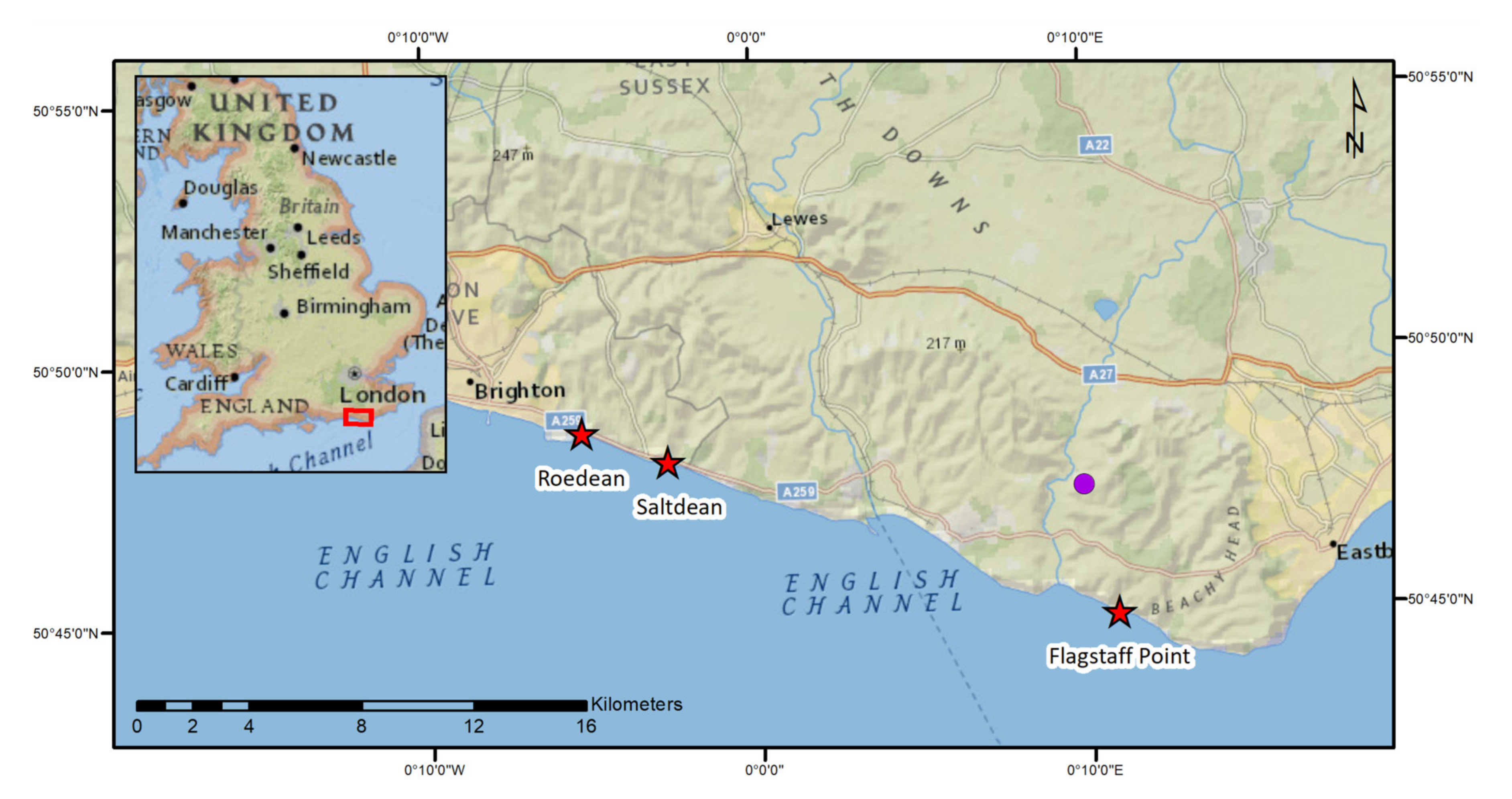
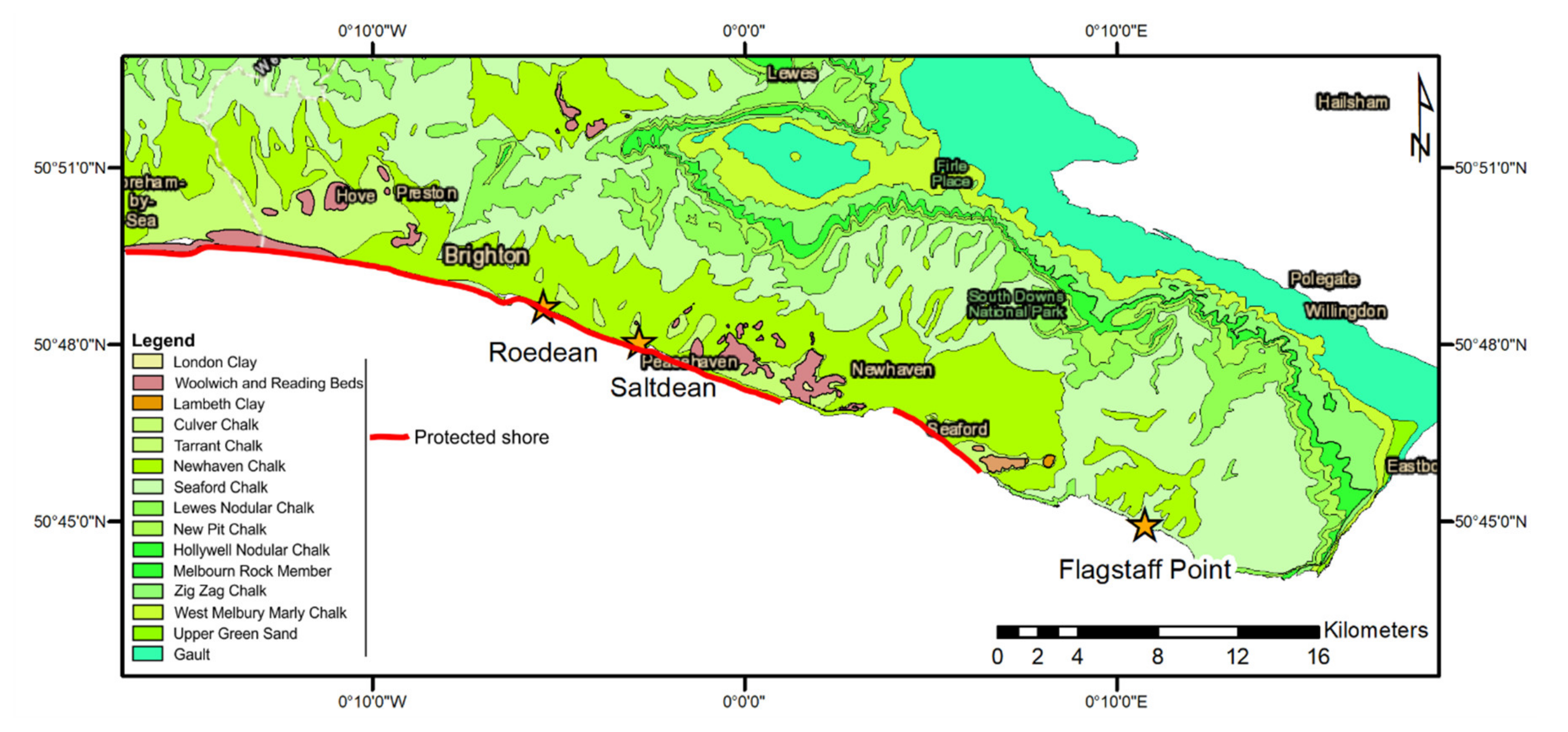
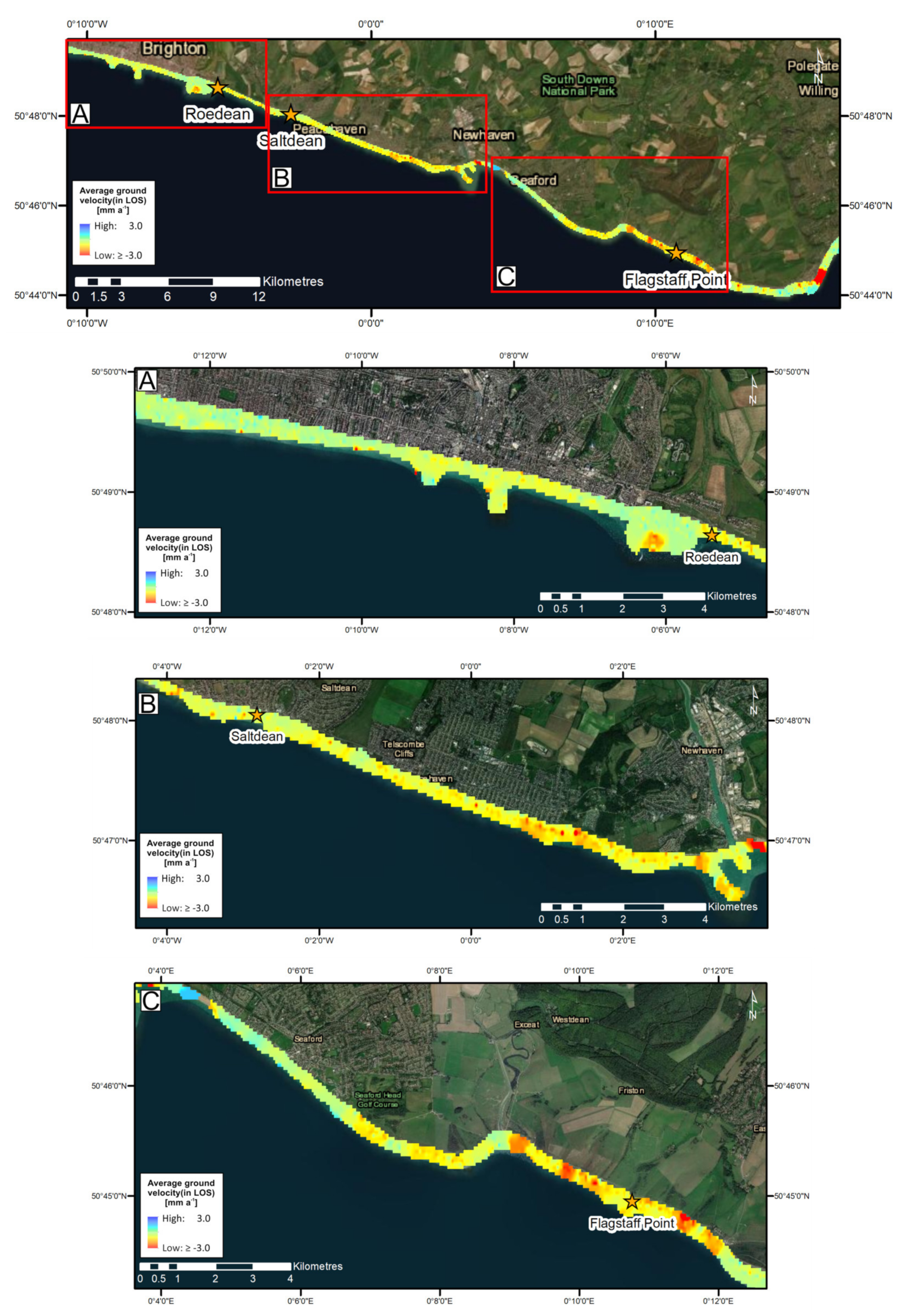
2. Study Region
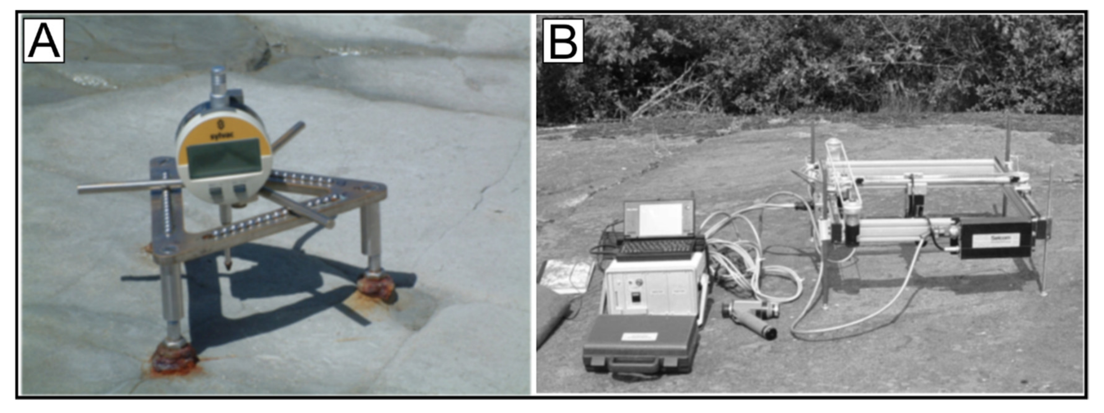
3. Existing Platform Downwearing Measuring Methods
4. Methods
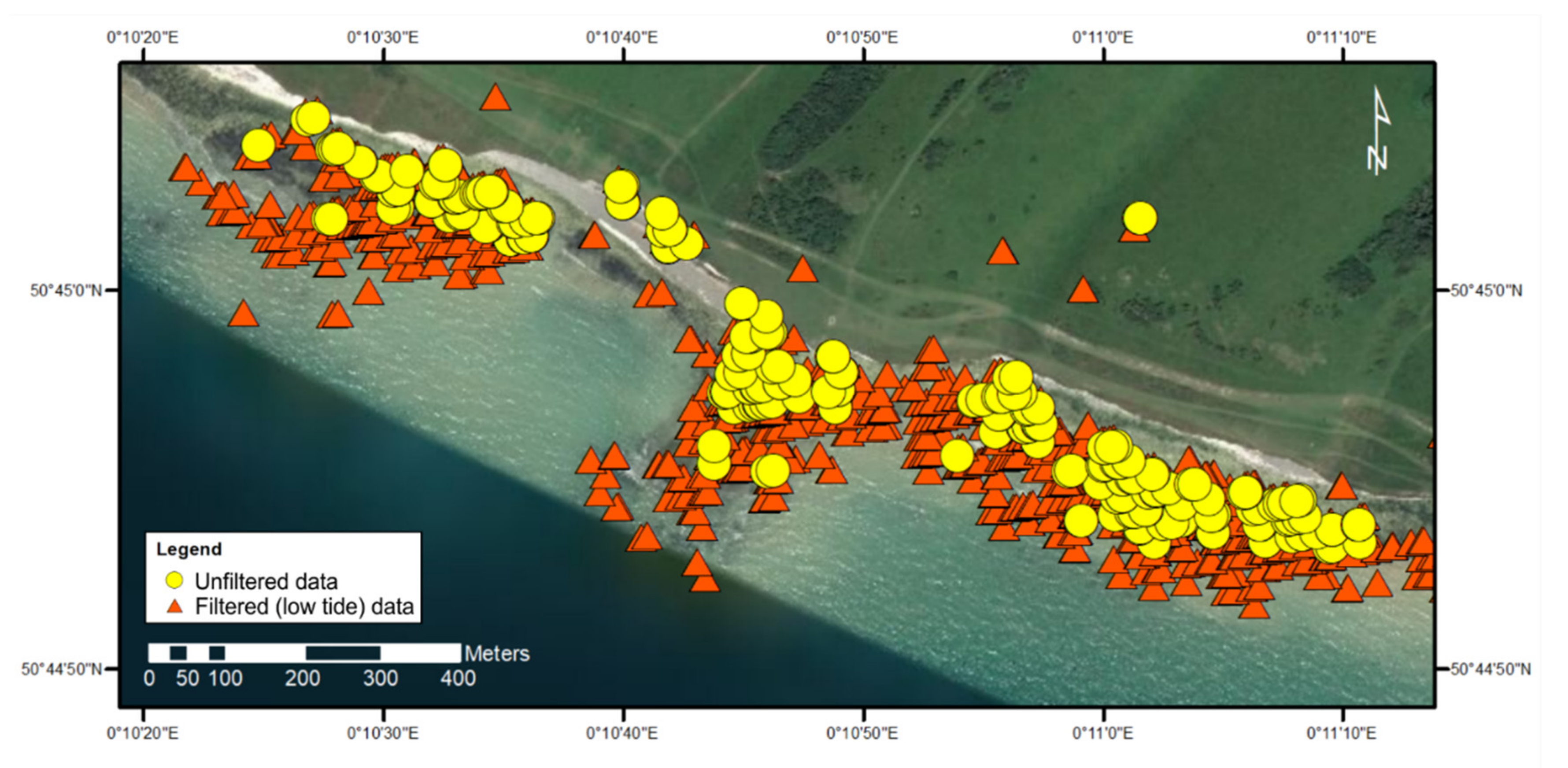
4.1. InSAR Methodology
4.2. Research Sites Chosen for Demonstration of Platform Downwearing
5. Results and Discussion
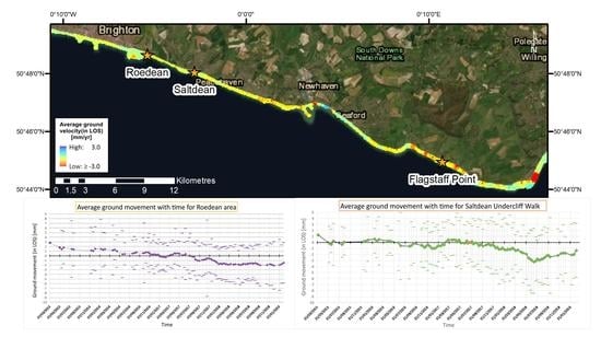
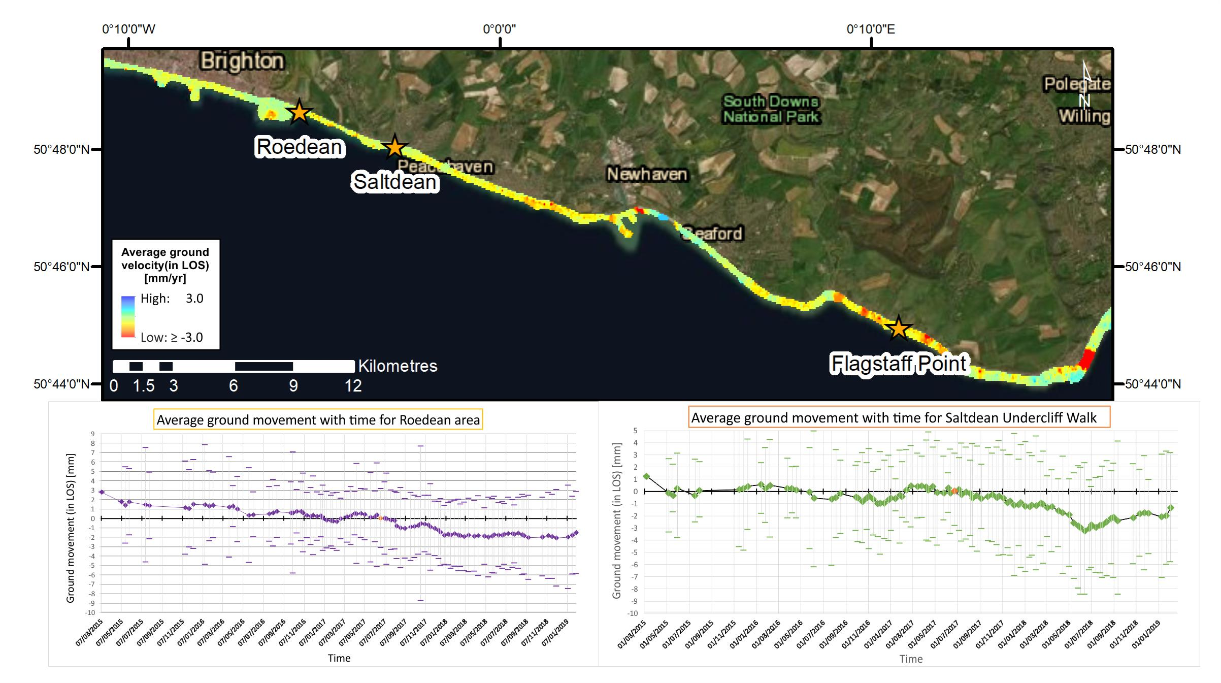
5.1. Regional Overview of the Results
Comparison with Previous Work
5.2. Analysis of Ground Level Change at the Research Sites
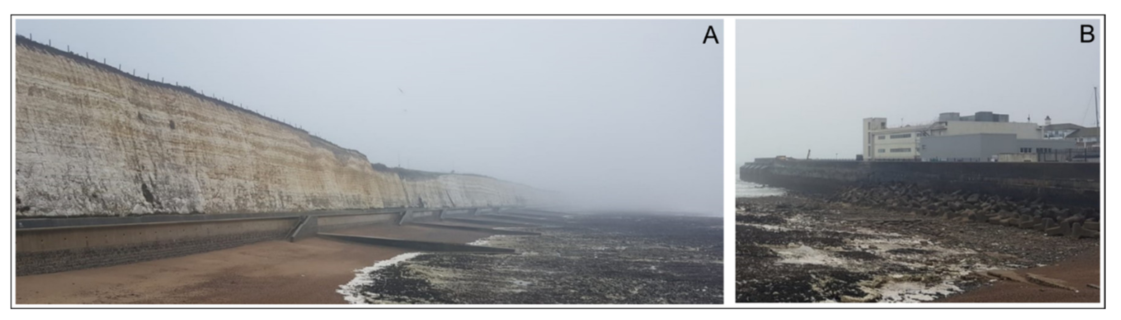
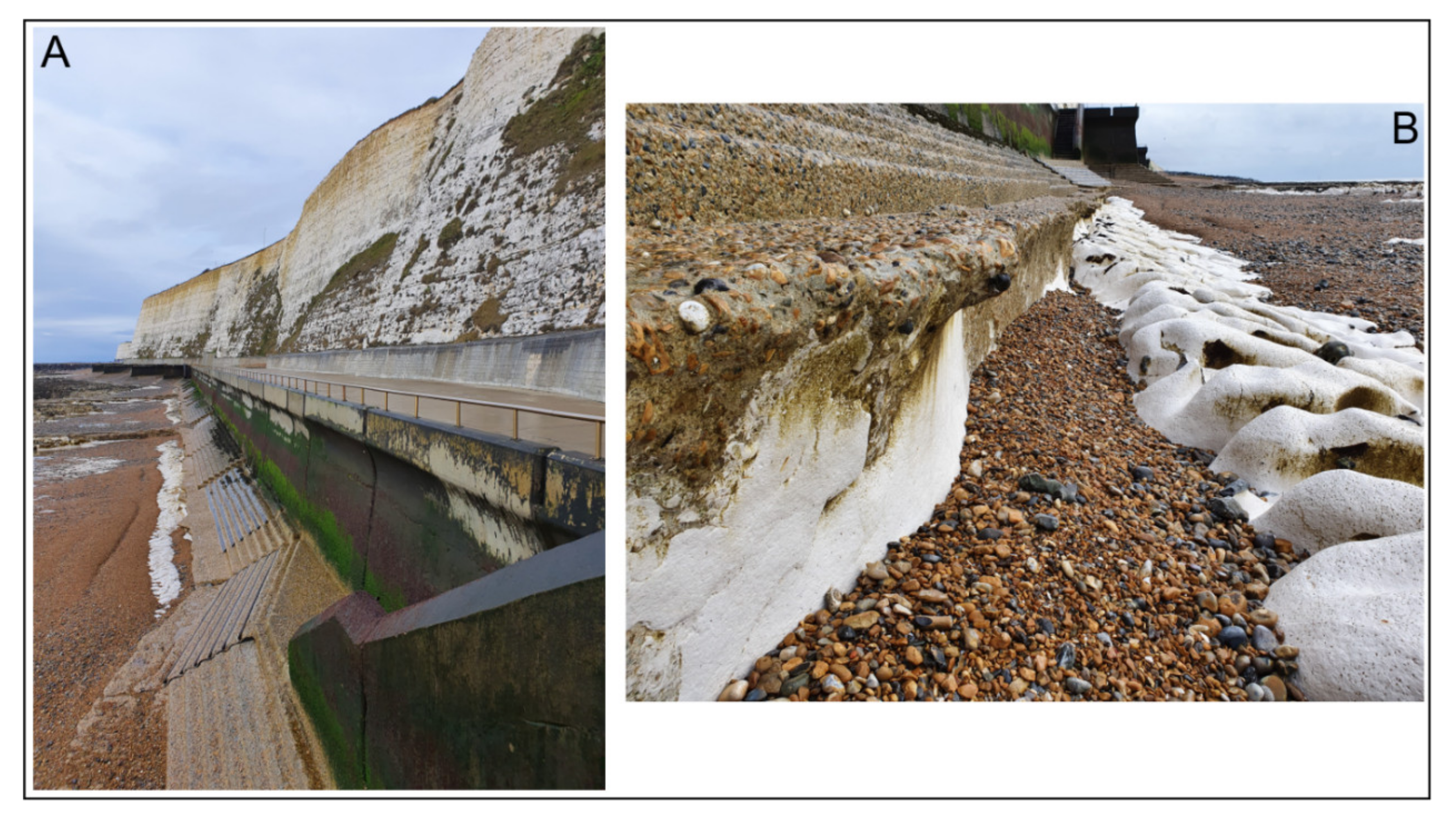
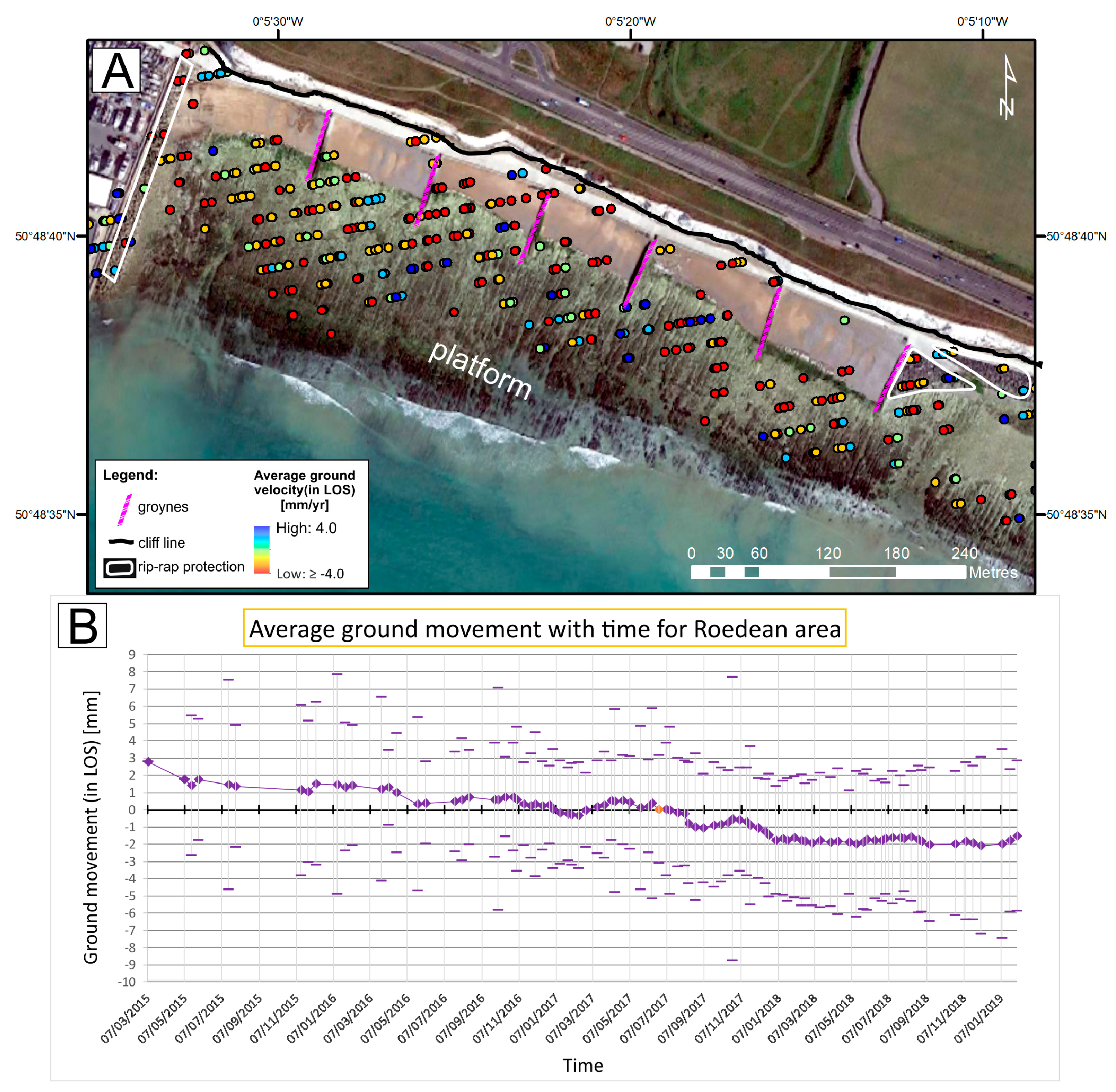
5.2.1. Roedean, East of Brighton Marina, Platform by Undercliff Walk
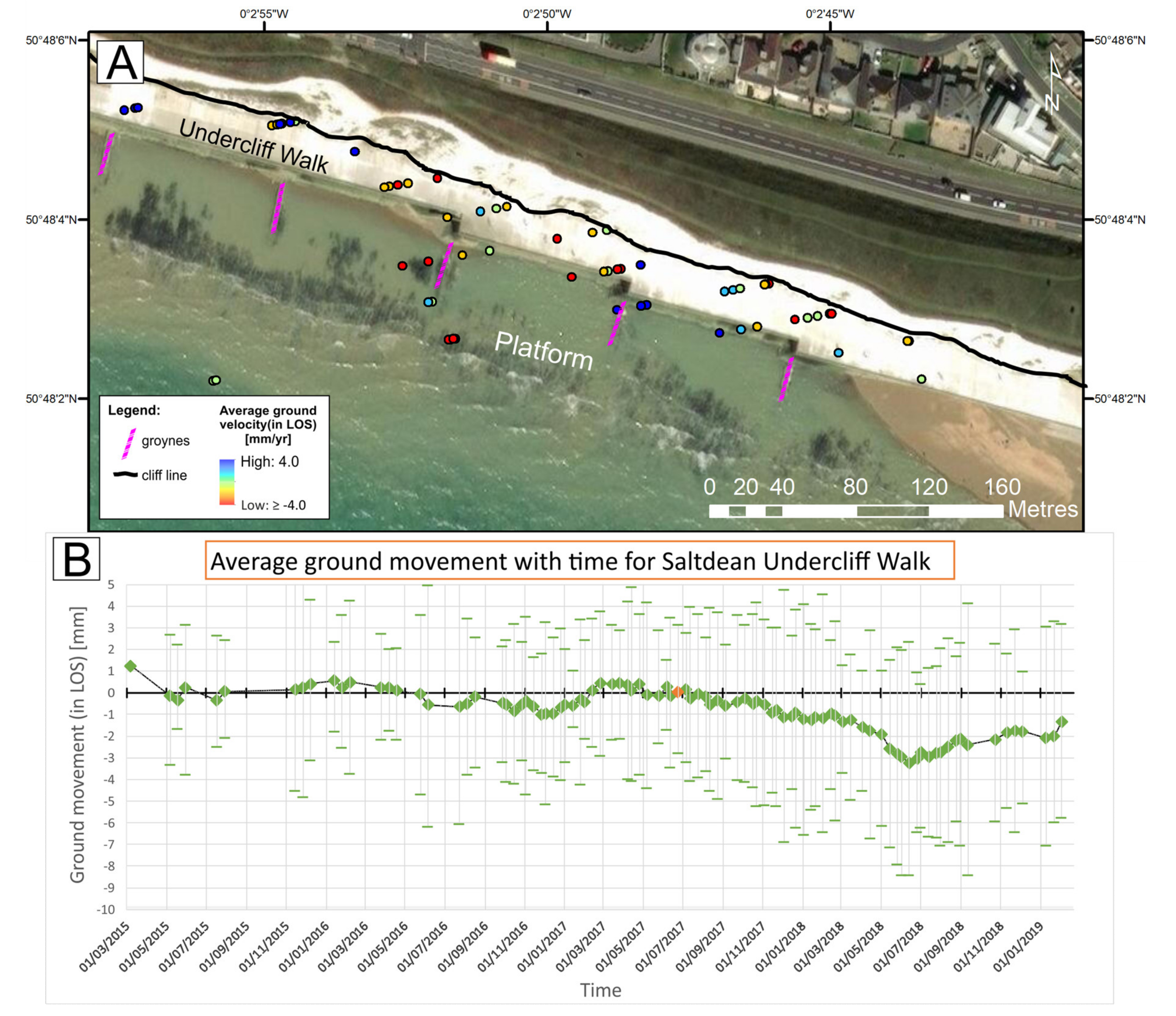
5.2.2. Saltdean
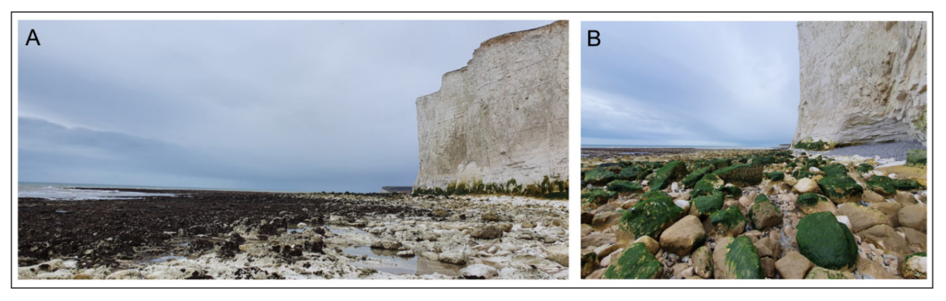
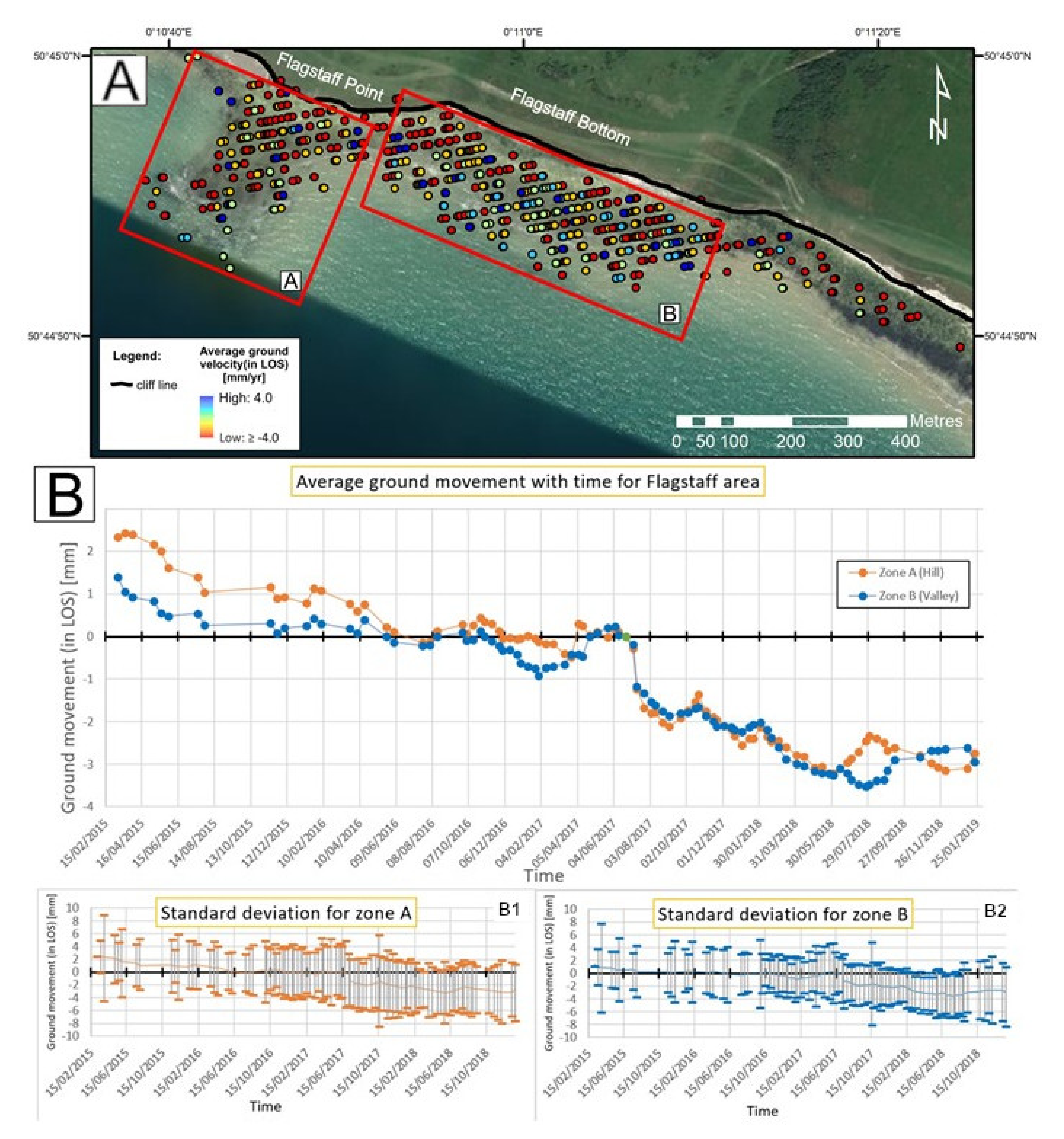
5.2.3. Seven Sisters Platform
6. Conclusions
Author Contributions
Funding
Acknowledgments
Conflicts of Interest
References
- Evans, E.; Ashley, R.; Hall, J.; Penning-Rowsell, E.; Sayers, P.; Thorne, C.; Watkinson, A. Foresight: Future Flooding: Scientific Summary: Volume I: Future Risks and Their Drivers; Government Office for Science: London, UK, 2004.
- Howard, T.; Palmer, M.; Guentchev, G.; Krijnen, J. Exploratory Sea Level Projections for the UK to 2300; Environment Agency: Bristol, UK, 2019; p. 98. [Google Scholar]
- Dornbusch, U.; Moses, C.; Robinson, D.A.; Williams, R. Soft copy photogrammetry to measure shore platform erosion on decadal timescales. J. Coast. Conserv. 2008, 11, 193–200. [Google Scholar] [CrossRef]
- Moses, C.; Robinson, D.; Barlow, J. Methods for measuring rock surface weathering and erosion: A critical review. Earth-Science Rev. 2014, 135, 141–161. [Google Scholar] [CrossRef]
- Cullen, N.D.; Verma, A.; Bourke, M.C. A comparison of structure from motion photogrammetry and the traversing micro-erosion meter for measuring erosion on shore platforms. Earth Surf. Dyn. 2018, 6, 1023–1039. [Google Scholar] [CrossRef]
- Swantesson, J.O.H. Recent microweathering phenomena in southern and central Sweden. Processes 1992, 3, 275–292. [Google Scholar] [CrossRef]
- BSI. BS 5930: 2015: Code of Practice for Ground Investigations; British Standards Institution: London, UK, 2015. [Google Scholar]
- Xue, F.; Lv, X.; Dou, F.; Yun, Y. A review of time-series Interferometric SAR techniques: A tutorial for surface deformation analysis. IEEE Geosci. Remote. Sens. Mag. 2020, 8, 22–42. [Google Scholar] [CrossRef]
- Massonnet, D.; Rossi, M.; Carmona, S. The displacement field of the Landers earthquake mapped by radar interferometry. Nat. Cell Biol. 1993, 364, 138–142. [Google Scholar] [CrossRef]
- Gabriel, A.K.; Goldstein, R.M.; Zebker, H.A. Mapping small elevation changes over large areas: Differential radar interferometry. J. Geophys. Res. Space Phys. 1989, 94, 9183. [Google Scholar] [CrossRef]
- Massironi, M.; Zampieri, D.; Bianchi, M.; Schiavo, A.; Franceschini, A. Use of PSInSAR™ data to infer active tectonics: Clues on the differential uplift across the Giudicarie belt (Central-Eastern Alps, Italy). Tectonophysics 2009, 476, 297–303. [Google Scholar] [CrossRef]
- Colesanti, C.; Wasowski, J. Investigating landslides with space-borne Synthetic Aperture Radar (SAR) interferometry. Eng. Geol. 2006, 88, 173–199. [Google Scholar] [CrossRef]
- Kiseleva, E.; Mikhailov, V.; Smolyaninova, E.; Dmitriev, P.; Golubev, V.; Timoshkina, E.; Hooper, A.; Samiei-Esfahany, S.; Hanssen, R. PS-InSAR monitoring of landslide activity in the black sea coast of the Caucasus. Procedia Technol. 2014, 16, 404–413. [Google Scholar] [CrossRef]
- Dong, J.; Zhang, L.; Tang, M.; Liao, M.; Xu, Q.; Gong, J.; Ao, M. Mapping landslide surface displacements with time series SAR interferometry by combining persistent and distributed scatterers: A case study of Jiaju landslide in Danba, China. Remote Sens. Environ. 2018, 205, 180–198. [Google Scholar] [CrossRef]
- Velasco, V.; Sanchez, C. Ground deformation mapping and monitoring of salt mines using InSAR technology. In Proceedings of the Solution Mining Research Institute Fall 2017 Technical Conference, Münster, Germany, 24–27 September 2017. [Google Scholar]
- Gonzáles-Martí, J.; Nevard, S.; Sánchez, J. The Use of InSAR (Interferometric Synthetic Aperture Radar) to Complement Control of Construction and Protect Third Party Assets; Crossrail Learning Legacy Report; Crossrail Ltd: London, UK, 2017. [Google Scholar]
- Giardina, G.; Milillo, G.; DeJong, M.; Perissin, D.; Milillo, G. Evaluation of InSAR monitoring data for post-tunnelling settlement damage assessment. Struct. Control Health Monit. 2018, 26, e2285. [Google Scholar] [CrossRef]
- Milillo, P.; Giardina, G.; DeJong, M.; Perissin, D.; Milillo, G. Multi-temporal InSAR structural damage assessment: The London crossrail case study. Remote. Sens. 2018, 10, 287. [Google Scholar] [CrossRef]
- Bischoff, C.A.; Ghail, R.C.; Mason, P.J.; Ferretti, A.; Davis, J.A. Photographic feature: Revealing millimetre-scale ground movements in London using SqueeSAR™. Q. J. Eng. Geol. Hydrogeol. 2019. [Google Scholar] [CrossRef]
- Scoular, J.; Croft, J.; Ghail, R.; Mason, P.J.; Lawrence, J.; Stoianov, I. Limitations of Persistent Scatterer Interferometry to measure small seasonal ground movements in an urban environment. Q. J. Eng. Geol. Hydrogeol. 2019, 53, 39–48. [Google Scholar] [CrossRef]
- Scoular, J.; Ghail, R.; Mason, P.J.; Lawrence, J.; Bellhouse, M.; Holley, R.; Morgan, T. Retrospective InSAR analysis of East London during the construction of the lee tunnel. Remote. Sens. 2020, 12, 849. [Google Scholar] [CrossRef]
- Ciampalini, A.; Solari, L.; Giannecchini, R.; Galanti, Y.; Moretti, S. Evaluation of subsidence induced by long-lasting buildings load using InSAR technique and geotechnical data: The case study of a Freight Terminal (Tuscany, Italy). Int. J. Appl. Earth Obs. Geoinf. 2019, 82, 82. [Google Scholar] [CrossRef]
- Sousa, J.J.; Ruiz, A.M.; Hanssen, R.F.; Bastos, L.; Gil, A.J.; Galindo-Zaldivar, J.; De Galdeano, C.S. PS-InSAR processing methodologies in the detection of field surface deformation—Study of the Granada basin (Central Betic Cordilleras, southern Spain). J. Geodyn. 2010, 49, 181–189. [Google Scholar] [CrossRef]
- Pratesi, F.; Tapete, D.; Del Ventisette, C.; Moretti, S. Mapping interactions between geology, subsurface resource exploitation and urban development in transforming cities using InSAR Persistent Scatterers: Two decades of change in Florence, Italy. Appl. Geogr. 2016, 77, 20–37. [Google Scholar] [CrossRef]
- Rohmer, J.; Raucoules, D. On the applicability of Persistent Scatterers Interferometry (PSI) analysis for long term CO2 storage monitoring. Eng. Geol. 2012, 147, 137–148. [Google Scholar] [CrossRef]
- Rohmer, J.; Loschetter, A.; Raucoules, D.; de Michele, M.; le Gallo, Y.; Raffard, D. Improving Persistent Scatterers Interferometry (PSI) analysis in highly vegetal/agricultural areas for long term CO2 storage monitoring. Energy Procedia 2014, 63, 4019–4026. [Google Scholar] [CrossRef][Green Version]
- Stavrou, A.; Lawrence, J.A.; Mortimore, R.N.; Murphy, W. A geotechnical and GIS based method for evaluating risk exposition along coastal cliff environments: A case study of the chalk cliffs of southern England. Nat. Hazards Earth Syst. Sci. 2011, 11, 2997–3011. [Google Scholar] [CrossRef]
- Moses, C.A. Chapter 4 The Rock Coast of the British Isles: Shore Platforms; Geological Society: London, UK, 2014; Volume 40, pp. 39–56. [Google Scholar]
- Lord, J.A.; Clayton, C.R.I.; Mortimore, R.N. Engineering in Chalk; CIRIA: London, UK, 2002. [Google Scholar]
- Mortimore, R.N. Logging the Chalk; Whittles Publishing: Caithness, Scotland, 2014; pp. 48–117. [Google Scholar]
- Lawrence, J.; Mortimore, R.; Stone, K.; Busby, J. Sea saltwater weakening of chalk and the impact on cliff instability. Geomorphology 2013, 191, 14–22. [Google Scholar] [CrossRef]
- Lawrence, J.; Spence, R.; Mortimore, R.N.; Eade, M.; Bottrell, S.H. Coastal cliff rock mass weakening of Chalk and the impact of salt water. Proc. Inst. Civ. Eng. Geotech. Eng. 2018, 171, 545–555. [Google Scholar] [CrossRef]
- Mider, G.; Lawrence, J. Anisotropic Permeability of Chalk, in Engineering in Chalk; ICE: London, UK, 2018; pp. 481–487. [Google Scholar]
- Mortimore, R.N.; Stone, K.J.; Lawrence, J.; Duperret, A. Chalk Physical Properties and Cliff Instability; Geological Society, London, Engineering Geology Special Publications: London, UK, 2004; Volume 20, pp. 75–88. [Google Scholar]
- Aliyu, M.M.; Murphy, W.; Lawrence, J.A.; Collier, R. Engineering geological characterization of flints. Q. J. Eng. Geol. Hydrogeol. 2017, 50, 133–147. [Google Scholar] [CrossRef]
- Robinson, L.A. The micro-erosion meter technique in a littoral environment. Mar. Geol. 1976, 22, M51–M58. [Google Scholar] [CrossRef]
- Stephenson, W.J.; Finlayson, B. Measuring erosion with the micro-erosion meter—Contributions to understanding landform evolution. Earth-Science Rev. 2009, 95, 53–62. [Google Scholar] [CrossRef]
- Swantesson, J.; Moses, C.; Berg, G.E.; Jansson, K. Methods for measuring shore platform micro erosion: A comparison of the micro-erosion meter and laser scanner. Z. fur Geomorphol. Suppl. 2006, 144, 1–17. [Google Scholar]
- Swantesson, J.O.H. Weathering and erosion of rock carvings in Sweden during the period 1994–2003—Micro mapping with laser scanner for assessment of breakdown rates. In Department of Physical Geology, Division for Environmental Sciences; Karlstad University: Karlstad, Sweden, 2005. [Google Scholar]
- Ellis, N. Morphology, Process and Rates of Denudation on the Chalk Shore Platform of East Sussex; Polytechnic: Brighton, UK, 1986. [Google Scholar]
- Dornbusch, U.; Robinson, D.A.; Williams, R.B.; Moses, C.A. Chalk shore platform erosion in the vicinity of sea defence structures and the impact of construction methods. Coast. Eng. 2007, 54, 801–810. [Google Scholar] [CrossRef]
- Dornbusch, U.; Robinson, D.A.; Williams, R.B.; Moses, C. Block removal and step backwearing as erosion processes on rock shore platforms: A preliminary case study of the chalk shore platforms of south-east England. Earth Surf. Process. Landf. 2010, 36, 661–671. [Google Scholar] [CrossRef]
- Ferretti, A.; Prati, C.; Rocca, F. Permanent scatterers in SAR interferometry. IEEE Trans. Geosci. Remote. Sens. 2001, 39, 8–20. [Google Scholar] [CrossRef]
- Crosetto, M.; Monserrat, O.; Cuevas-González, M.; Devanthéry, N.; Crippa, B. Persistent scatterer interferometry: A review. ISPRS J. Photogramm. Remote. Sens. 2016, 115, 78–89. [Google Scholar] [CrossRef]
- Ferretti, A.; Monti-Guarnieri, A.; Prati, C.; Rocca, F.; Massonet, D. InSAR Principles: Guidelines for SAR Interferometry Processing and Interpretation; Fletcher, K., Ed.; ESA Publications: Noordwijk, The Netherlands, 2007. [Google Scholar]
- Crosetto, M.; Monserrat, O.; Jungner, A.; Crippa, B. Persistent scatterer interferometry: Potential and limits. In Proceedings of the 2009 ISPRS Workshop on High-Resolution Earth Imaging for Geospatial Information, Hannover, Germany, 2–5 June 2009. [Google Scholar]


| Location | Grid Reference | Photogrammetry [mm a−1] | MEM Measurements [mm a−1] | Laser Scanning [mm a−1] |
|---|---|---|---|---|
| Roedean | TQ 34667 03136 | −0.9 to −0.1 | −3.5 | |
| Peacehaven | TQ 41207 01477 | −4.9 to −1.0 | −1.5 | −0.3 |
| Hope Gap | TV 51041 97373 | −20 to −6 |
| Formation Name | Average Velocity [mm a−1] | Number of Points Analysed | Type of Area |
|---|---|---|---|
| Newhaven Chalk | −0.40 | 36,824 | Protected |
| Seaford Chalk | −0.66 | 3788 | Unprotected |
| Lewes Nodular Chalk | −0.53 | 1811 | Unprotected |
| Location | Grid Reference | Photogrammetry [mm a−1] | MEM Measurements [mm a−1] | Laser Scanning [mm a−1] | InSAR [mm a−1] |
|---|---|---|---|---|---|
| Roedean | TQ 34667 03136 | −0.9 to −0.1 | −3.5 | −1.0 | |
| Peacehaven | TQ 41207 01477 | −4.9 to −1.0 | −1.5 | −0.3 | −1.27 |
| Hope Gap | TV 51041 97373 | −20 to −6 | −0.61 |
© 2020 by the authors. Licensee MDPI, Basel, Switzerland. This article is an open access article distributed under the terms and conditions of the Creative Commons Attribution (CC BY) license (http://creativecommons.org/licenses/by/4.0/).
Share and Cite
Mider, G.; Lawrence, J.; Mason, P.; Ghail, R. Monitoring Littoral Platform Downwearing Using Differential SAR Interferometry. Remote Sens. 2020, 12, 3243. https://doi.org/10.3390/rs12193243
Mider G, Lawrence J, Mason P, Ghail R. Monitoring Littoral Platform Downwearing Using Differential SAR Interferometry. Remote Sensing. 2020; 12(19):3243. https://doi.org/10.3390/rs12193243
Chicago/Turabian StyleMider, Gosia, James Lawrence, Philippa Mason, and Richard Ghail. 2020. "Monitoring Littoral Platform Downwearing Using Differential SAR Interferometry" Remote Sensing 12, no. 19: 3243. https://doi.org/10.3390/rs12193243
APA StyleMider, G., Lawrence, J., Mason, P., & Ghail, R. (2020). Monitoring Littoral Platform Downwearing Using Differential SAR Interferometry. Remote Sensing, 12(19), 3243. https://doi.org/10.3390/rs12193243