Leaf Nitrogen Concentration and Plant Height Prediction for Maize Using UAV-Based Multispectral Imagery and Machine Learning Techniques
 ,
,  ,
,  ,
, 
 ,
,  ,
,  ,
,  and
and 
Abstract
1. Introduction
2. Materials and Methods
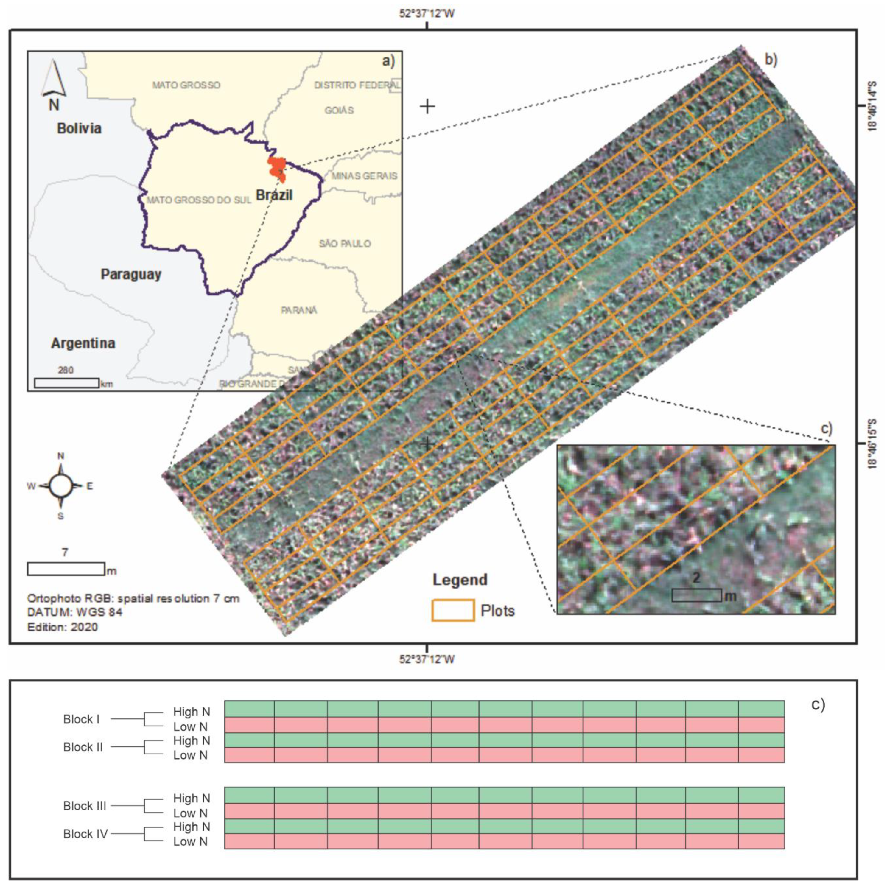
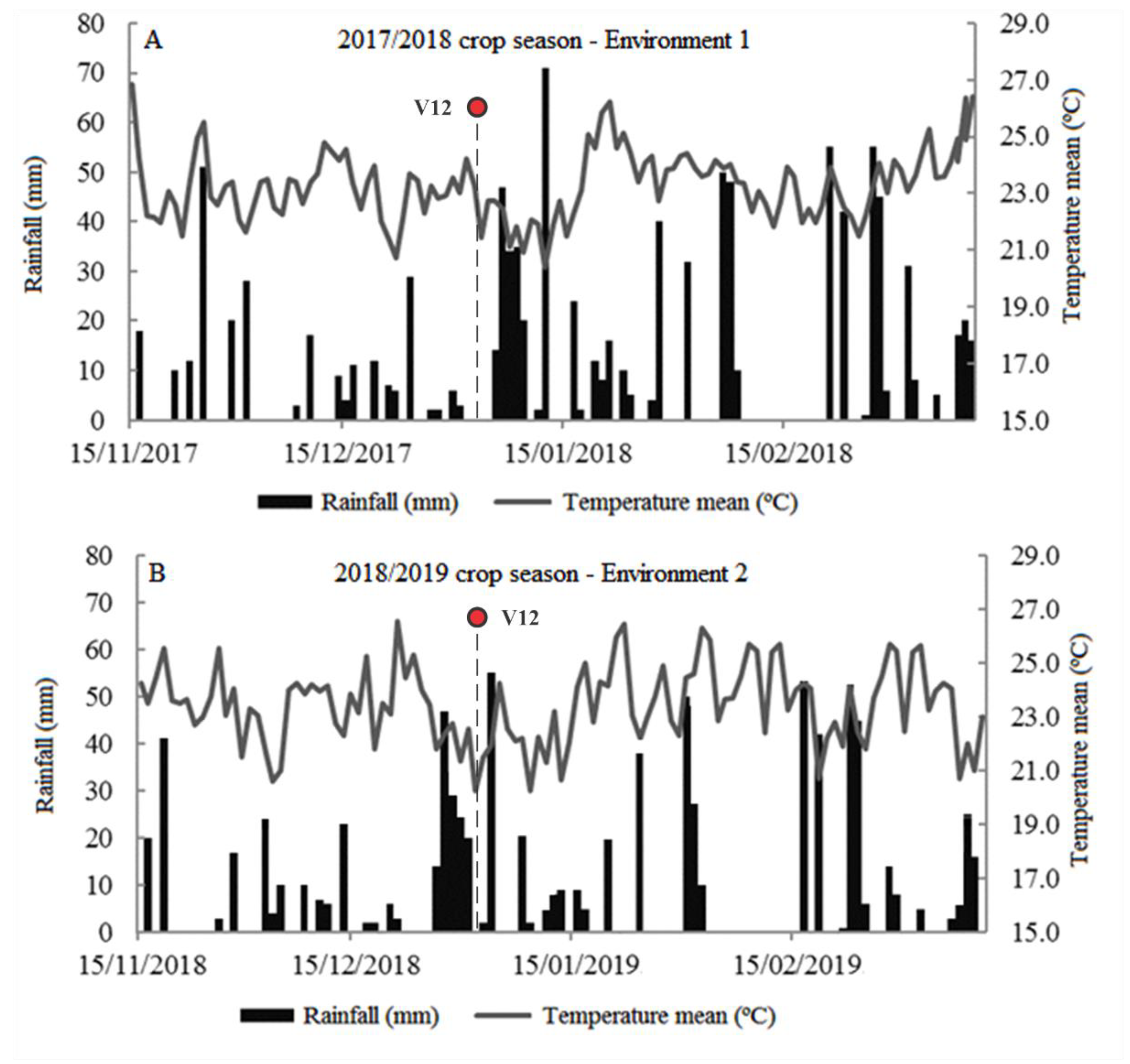
2.1. Field Trials
2.2. Evaluated Variables
2.3. Image Acquisition and Vegetation Indices
2.4. Data Analysis
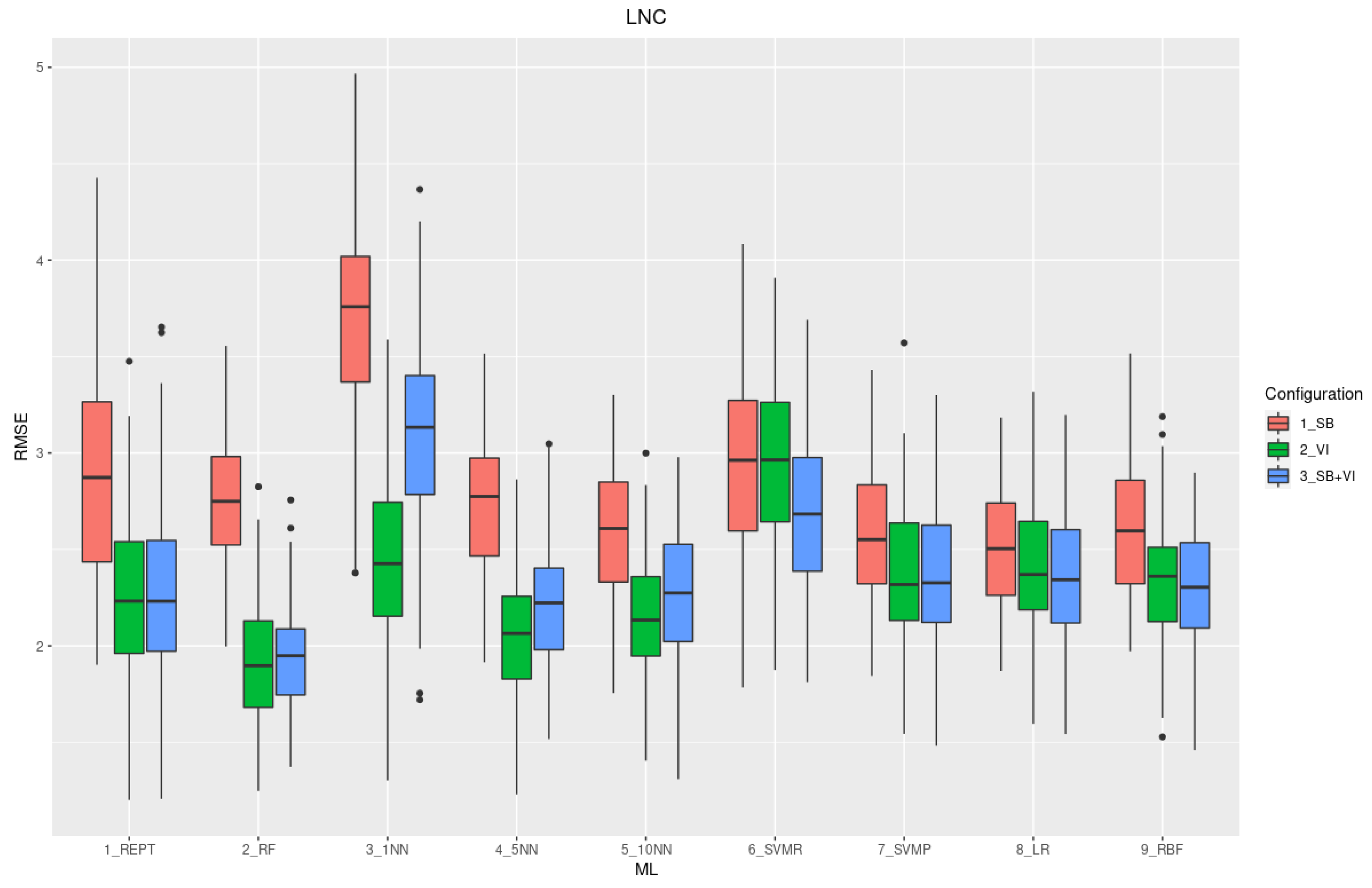
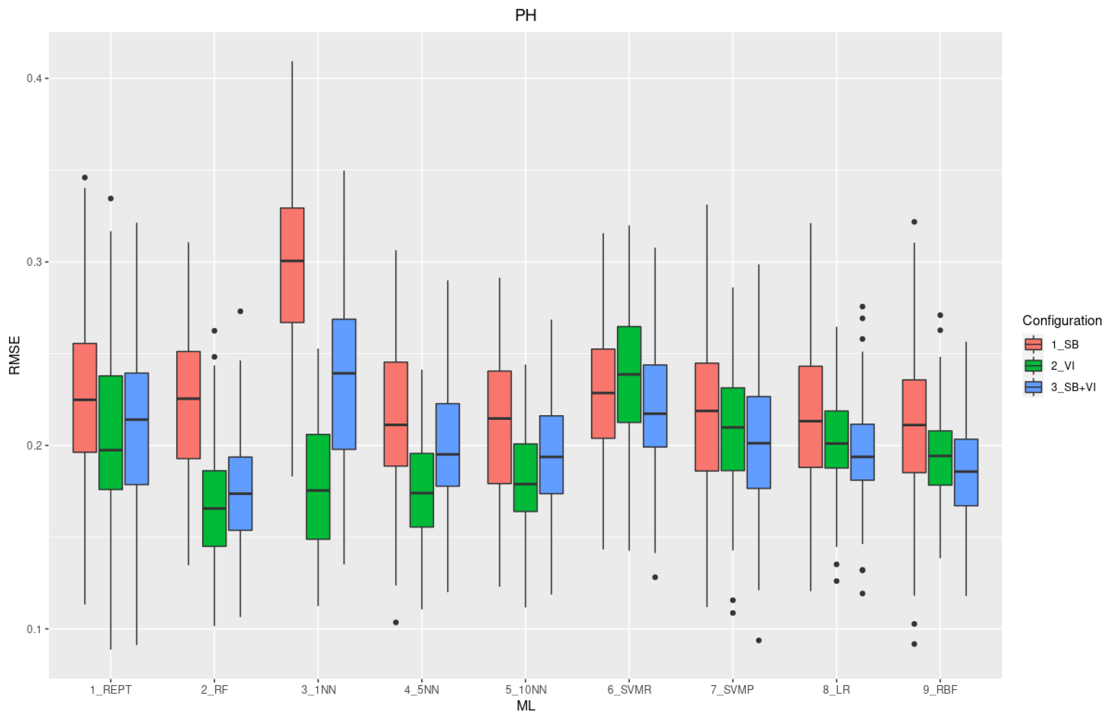
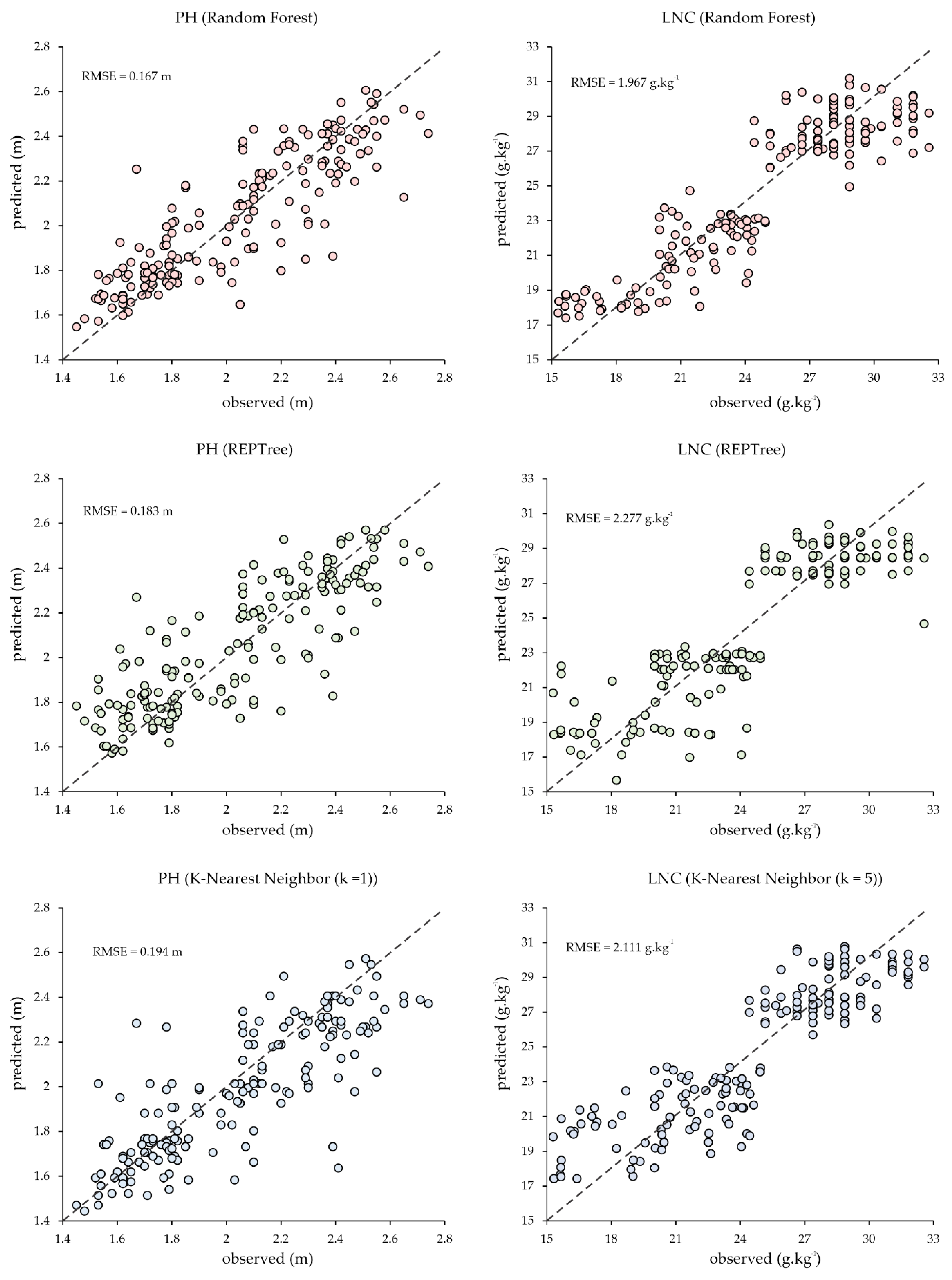
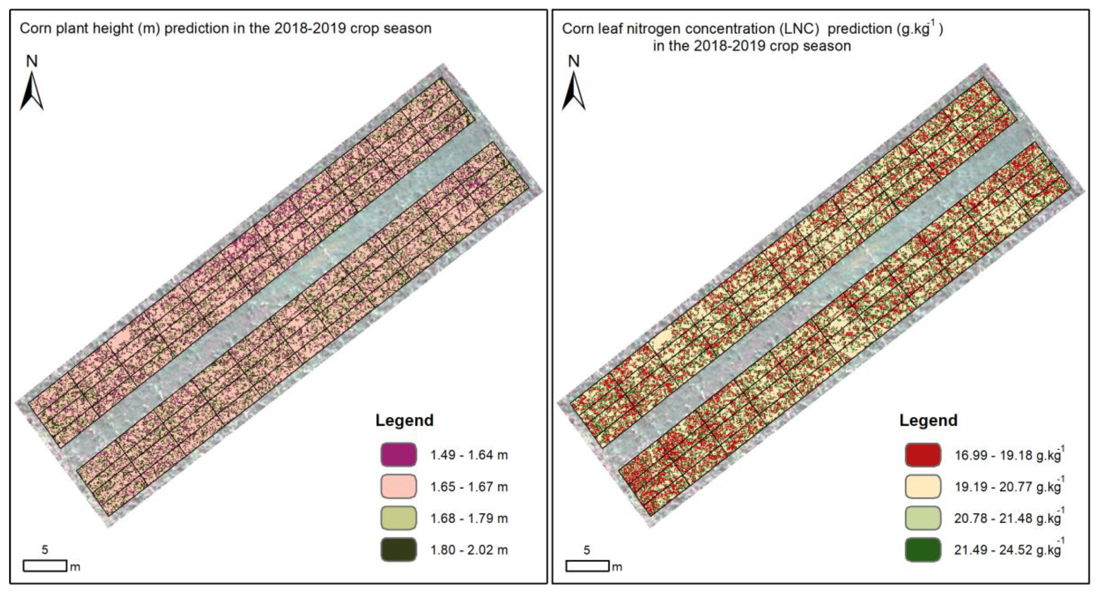
3. Results
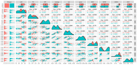
3.1. Relationship among the Agronomic Variables
3.2. Models’ Performances for LNC and PH Prediction
4. Discussion
5. Conclusions
Author Contributions
Funding
Acknowledgments
Conflicts of Interest
References
- Weiss, M.; Jacob, F.; Duveiller, G. Remote sensing for agricultural applications: A meta-review. Remote Sens. Environ. 2020, 236, 111402. [Google Scholar] [CrossRef]
- Wang, S.; Azzari, G.; Lobell, D.B. Crop type mapping without field-level labels: Random forest transfer and unsupervised clustering techniques. Remote Sens. Environ. 2019, 222, 303–317. [Google Scholar] [CrossRef]
- Hunt, E.R.; Daughtry, C.S.T. What good are unmanned aircraft systems for agricultural remote sensing and precision agriculture? Int. J. Remote Sens. 2018, 39, 5345–5376. [Google Scholar] [CrossRef]
- Zhong, L.; Hu, L.; Zhou, H. Deep learning based multi-temporal crop classification. Remote Sens. Environ. 2019, 221, 430–443. [Google Scholar] [CrossRef]
- Haghverdi, A.; Washington-Allen, R.A.; Leib, B.G. Prediction of cotton lint yield from phenology of crop indices using artificial neural networks. Comput. Electron. Agric. 2018, 152, 186–197. [Google Scholar] [CrossRef]
- Chen, S.W.; Shivakumar, S.S.; Dcunha, S.; Das, J.; Okon, E.; Qu, C.; Taylor, C.J.; Kumar, V. Counting Apples and Oranges with Deep Learning: A Data-Driven Approach. IEEE Robot. Autom. Lett. 2017, 2, 781–788. [Google Scholar] [CrossRef]
- Hunt, M.L.; Blackburn, G.A.; Carrasco, L.; Redhead, J.W.; Rowland, C.S. High resolution wheat yield mapping using Sentinel-2. Remote Sens. Environ. 2019, 233, 111410. [Google Scholar] [CrossRef]
- Jin, Z.; Azzari, G.; You, C.; Di Tommaso, S.; Aston, S.; Burke, M.; Lobell, D.B. Smallholder maize area and yield mapping at national scales with Google Earth Engine. Remote Sens. Environ. 2019, 228, 115–128. [Google Scholar] [CrossRef]
- Sun, J.; Di, L.; Sun, Z.; Shen, Y.; Lai, Z. County-level soybean yield prediction using deep CNN-LSTM model. Sensors 2019, 19, 4363. [Google Scholar] [CrossRef]
- Delloye, C.; Weiss, M.; Defourny, P. Retrieval of the canopy chlorophyll content from Sentinel-2 spectral bands to estimate nitrogen uptake in intensive winter wheat cropping systems. Remote Sens. Environ. 2018, 216, 245–261. [Google Scholar] [CrossRef]
- Osco, L.P.; Marques Ramos, A.P.; Saito Moriya, É.A.; de Souza, M.; Marcato Junior, J.; Matsubara, E.T.; Imai, N.N.; Creste, J.E. Improvement of leaf nitrogen content inference in Valencia-orange trees applying spectral analysis algorithms in UAV mounted-sensor images. Int. J. Appl. Earth Obs. Geoinf. 2019, 83, 101907. [Google Scholar] [CrossRef]
- Osco, L.P.; Ramos, A.P.M.; Pinheiro, M.M.F.; Moriya, É.A.S.; Imai, N.N.; Estrabis, N.; Ianczyk, F.; de Araújo, F.F.; Liesenberg, V.; de Castro Jorge, L.A.; et al. A machine learning approach to predict nutrient content in valencia-orange leaf hyperspectral measurements. Remote Sens. 2020, 12, 906. [Google Scholar] [CrossRef]
- Song, Y.; Wang, J. Soybean canopy nitrogen monitoring and prediction using ground based multispectral remote sensors. In Proceedings of the 2016 IEEE International Geoscience and Remote Sensing Symposium (IGARSS), Beijing, China, 10–15 July 2016; pp. 6389–6392. [Google Scholar] [CrossRef]
- Cammarano, D.; Fitzgerald, G.J.; Casa, R.; Basso, B. Assessing the robustness of vegetation indices to estimate wheat N in mediterranean environments. Remote Sens. 2014, 6, 2827–2844. [Google Scholar] [CrossRef]
- Xue, J.; Gao, S.; Fan, Y.; Li, L.; Ming, B.; Wang, K.; Xie, R.; Hou, P.; Li, S. Traits of plant morphology, stalk mechanical strength, and biomass accumulation in the selection of lodging-resistant maize cultivars. Eur. J. Agron. 2020, 117, 126073. [Google Scholar] [CrossRef]
- Cilia, C.; Panigada, C.; Rossini, M.; Meroni, M.; Busetto, L.; Amaducci, S.; Boschetti, M.; Picchi, V.; Colombo, R. Nitrogen status assessment for variable rate fertilization in maize through hyperspectral imagery. Remote Sens. 2014, 6, 6549–6565. [Google Scholar] [CrossRef]
- Wang, J.; Shen, C.; Liu, N.; Jin, X.; Fan, X.; Dong, C.; Xu, Y. Non-Destructive evaluation of the leaf nitrogen concentration by In-Field visible/Near-Infrared spectroscopy in pear orchards. Sensors 2017, 17, 538. [Google Scholar] [CrossRef]
- Prado Osco, L.; Marques Ramos, A.P.; Roberto Pereira, D.; Akemi Saito Moriya, É.; Nobuhiro Imai, N.; Takashi Matsubara, E.; Estrabis, N.; de Souza, M.; Marcato Junior, J.; Gonçalves, W.N.; et al. Predicting canopy nitrogen content in citrus-trees using random forest algorithm associated to spectral vegetation indices from UAV-imagery. Remote Sens. 2019, 11, 2925. [Google Scholar] [CrossRef]
- Muñoz-Huerta, R.F.; Guevara-Gonzalez, R.G.; Contreras-Medina, L.M.; Torres-Pacheco, I.; Prado-Olivarez, J.; Ocampo-Velazquez, R.V. A review of methods for sensing the nitrogen status in plants: Advantages, disadvantages and recent advances. Sensors 2013, 13, 10823–10843. [Google Scholar] [CrossRef]
- O’Connell, J.L.; Byrd, K.B.; Kelly, M. Remotely-sensed indicators of N-related biomass allocation in Schoenoplectus acutus. PLoS ONE 2014, 9. [Google Scholar] [CrossRef]
- Zheng, H.; Li, W.; Jiang, J.; Liu, Y.; Cheng, T.; Tian, Y.; Zhu, Y.; Cao, W.; Zhang, Y.; Yao, X. A comparative assessment of different modeling algorithms for estimating leaf nitrogen content in winter wheat using multispectral images from an unmanned aerial vehicle. Remote Sens. 2018, 10, 2026. [Google Scholar] [CrossRef]
- Raper, T.B.; Varco, J.J. Canopy-scale wavelength and vegetative index sensitivities to cotton growth parameters and nitrogen status. Precis. Agric. 2014, 16, 62–76. [Google Scholar] [CrossRef]
- Brinkhoff, J.; Dunn, B.W.; Robson, A.J.; Dunn, T.S.; Dehaan, R.L. Modeling mid-season rice nitrogen uptake using multispectral satellite data. Remote Sens. 2019, 11, 1837. [Google Scholar] [CrossRef]
- Liu, Y.L.; Lyu, Q.; He, S.L.; Yi, S.L.; Liu, X.F.; Xie, R.J.; Zheng, Y.; Deng, L. Prediction of nitrogen and phosphorus contents in citrus leaves based on hyperspectral imaging. Int. J. Agric. Biol. Eng. 2015, 8, 80–88. [Google Scholar] [CrossRef]
- He, L.; Song, X.; Feng, W.; Guo, B.B.; Zhang, Y.S.; Wang, Y.H.; Wang, C.Y.; Guo, T.C. Improved remote sensing of leaf nitrogen concentration in winter wheat using multi-angular hyperspectral data. Remote Sens. Environ. 2016, 174, 122–133. [Google Scholar] [CrossRef]
- Miyoshi, G.T.; Arruda, M.D.; Osco, L.P.; Marcato Junior, J.; Gonçalves, D.N.; Imai, N.N.; Tommaselli, A.M.; Honkavaara, E.; Gonçalves, W.N. A novel deep learning method to identify single tree species in UAV-based hyperspectral images. Remote Sens. 2020, 12, 1294. [Google Scholar] [CrossRef]
- Maxwell, A.E.; Warner, T.A.; Fang, F. Implementation of machine-learning classification in remote sensing: An applied review. Int. J. Remote Sens. 2018, 39, 2784–2817. [Google Scholar] [CrossRef]
- Singh, A.; Ganapathysubramanian, B.; Singh, A.K.; Sarkar, S. Machine Learning for High-Throughput Stress Phenotyping in Plants. Trends Plant Sci. 2016, 21, 110–124. [Google Scholar] [CrossRef]
- Ball, J.E.; Anderson, D.T.; Chan, C.S. Comprehensive survey of deep learning in remote sensing: Theories, tools, and challenges for the community. J. Appl. Remote Sens. 2017, 11, 1. [Google Scholar] [CrossRef]
- Osco, L.P.; Ramos, A.P.M.; Moriya, É.A.S.; Bavaresco, L.G.; de Lima, B.C.; Estrabis, N.; Pereira, D.R.; Creste, J.E.; Júnior, J.M.; Gonçalves, W.N.; et al. Modeling hyperspectral response of water-stress induced lettuce plants using artificial neural networks. Remote Sens. 2019, 11, 2797. [Google Scholar] [CrossRef]
- Berger, K.; Verrelst, J.; Féret, J.B.; Wang, Z.; Wocher, M.; Strathmann, M.; Danner, M.; Mauser, W.; Hank, T. Crop nitrogen monitoring: Recent progress and principal developments in the context of imaging spectroscopy missions. Remote Sens. Environ. 2020, 242, 111758. [Google Scholar] [CrossRef]
- Zha, H.; Miao, Y.; Wang, T.; Li, Y.; Zhang, J.; Sun, W. Improving Unmanned Aerial Vehicle Remote Sensing-Based Rice Nitrogen Nutrition Index Prediction with Machine Learning. Remote Sens. 2020, 12, 215. [Google Scholar] [CrossRef]
- Chlingaryan, A.; Sukkarieh, S.; Whelan, B. Machine learning approaches for crop yield prediction and nitrogen status estimation in precision agriculture: A review. Comput. Electron. Agric. 2018, 151, 61–69. [Google Scholar] [CrossRef]
- Han, L.; Yang, G.; Dai, H.; Xu, B.; Yang, H.; Feng, H.; Li, Z.; Yang, X. Modeling maize above-ground biomass based on machine learning approaches using UAV remote-sensing data. Plant Methods 2019, 15, 1–19. [Google Scholar] [CrossRef] [PubMed]
- Yang, N.; Liu, D.; Feng, Q.; Xiong, Q.; Zhang, L.; Ren, T.; Zhao, Y.; Zhu, D.; Huang, J. Large-scale crop mapping based on machine learning and parallel computation with grids. Remote Sens. 2019, 11, 1500. [Google Scholar] [CrossRef]
- Sharma, L.K.; Bu, H.; Franzen, D.W.; Denton, A. Use of corn height measured with an acoustic sensor improves yield estimation with ground based active optical sensors. Comput. Electron. Agric. 2016, 124, 254–262. [Google Scholar] [CrossRef]
- Jiang, T.; Liu, J.; Gao, Y.; Sun, Z.; Chen, S.; Yao, N.; Ma, H.; Feng, H.; Yu, Q.; He, J. Simulation of plant height of winter wheat under soil Water stress using modified growth functions. Agric. Water Manag. 2020, 232, 106066. [Google Scholar] [CrossRef]
- Almeida, V.C.; Viana, J.M.S.; DeOliveira, H.M.; Risso, L.A.; Ribeiro, A.F.S.; DeLima, R.O. Genetic diversity and path analysis for nitrogen use efficiency of tropical popcorn (Zea mays ssp. everta) inbred lines in adult stage. Plant Breed. 2018, 137, 839–847. [Google Scholar] [CrossRef]
- Torres, L.G.; Rodrigues, M.C.; Lima, N.L.; Horta Trindade, T.F.; Fonseca e Silva, F.; Azevedo, C.F.; DeLima, R.O. Multi-trait multi-environment Bayesian model reveals g x e interaction for nitrogen use efficiency components in tropical maize. PLoS ONE 2018, 13, e0199492. [Google Scholar] [CrossRef]
- Silva, F.C. Da Manual de Análises Químicas de Solos, Plantas e Fertilizantes; Fernando do Amaral Pereira, 2nd ed.; Embrapa Informação Tecnológica: Brasilia, Brazil, 2009. [Google Scholar]
- Rouse, J.W.; Hass, R.H.; Schell, J.A.; Deering, D.W. Monitoring vegetation systems in the great plains with ERTS. Third Earth Resour. Technol. Satell. Symp. 1973, 1, 309–317. [Google Scholar]
- Gitelson, A.; Merzlyak, M.N. Quantitative estimation of chlorophyll-a using reflectance spectra: Experiments with autumn chestnut and maple leaves. J. Photochem. Photobiol. B Biol. 1994, 22, 247–252. [Google Scholar] [CrossRef]
- Gitelson, A.A.; Kaufman, Y.J.; Merzlyak, M.N. Use of a green channel in remote sensing of global vegetation from EOS- MODIS. Remote Sens. Environ. 1996, 58, 289–298. [Google Scholar] [CrossRef]
- Huete, A.R. A Soil-Adjusted Vegetation Index (SAVI). Remote Sens. Environ. 1988, 25, 295–309. [Google Scholar] [CrossRef]
- Mitchell, T.M. Machine Learning, 1st ed.; McGraw-Hill, Inc.: New York, NY, USA, 1997. [Google Scholar]
- Saha, S.; Saha, M.; Mukherjee, K.; Arabameri, A.; Ngo, P.T.T.; Paul, G.C. Predicting the deforestation probability using the binary logistic regression, random forest, ensemble rotational forest, REPTree: A case study at the Gumani River Basin, India. Sci. Total Environ. 2020, 730, 139197. [Google Scholar] [CrossRef] [PubMed]
- Belgiu, M.; Drăgu, L. Random forest in remote sensing: A review of applications and future directions. ISPRS J. Photogramm. Remote Sens. 2016, 114, 24–31. [Google Scholar] [CrossRef]
- Ali, N.; Neagu, D.; Trundle, P. Evaluation of k-nearest neighbour classifier performance for heterogeneous data sets. SN Appl. Sci. 2019, 1, 1–15. [Google Scholar] [CrossRef]
- Nalepa, J.; Kawulok, M. Selecting training sets for support vector machines: A review. Artif. Intell. Rev. 2019, 52, 857–900. [Google Scholar] [CrossRef]
- Štepanovský, M.; Ibrová, A.; Buk, Z.; Velemínská, J. Novel age estimation model based on development of permanent teeth compared with classical approach and other modern data mining methods. Forensic Sci. Int. 2017, 279, 72–82. [Google Scholar] [CrossRef]
- Cheshmberah, F.; Fathizad, H.; Parad, G.A.; Shojaeifar, S. Comparison of RBF and MLP neural network performance and regression analysis to estimate carbon sequestration. Int. J. Environ. Sci. Technol. 2020. [Google Scholar] [CrossRef]
- Kross, A.; McNairn, H.; Lapen, D.; Sunohara, M.; Champagne, C. Assessment of RapidEye vegetation indices for estimation of leaf area index and biomass in corn and soybean crops. Int. J. Appl. Earth Obs. Geoinf. 2015, 34, 235–248. [Google Scholar] [CrossRef]
- Varela, S.; Dhodda, P.R.; Hsu, W.H.; Prasad, P.V.V.; Assefa, Y.; Peralta, N.R.; Griffin, T.; Sharda, A.; Ferguson, A.; Ciampitti, I.A. Early-season stand count determination in Corn via integration of imagery from unmanned aerial systems (UAS) and supervised learning techniques. Remote Sens. 2018, 10, 343. [Google Scholar] [CrossRef]
- Miphokasap, P.; Wannasiri, W. Estimations of Nitrogen Concentration in sugarcane using hyperspectral imagery. Sustainability. 2018, 10, 1266. [Google Scholar] [CrossRef]
- Abdel-Rahman, E.M.; Ahmed, F.B.; Ismail, R. Random forest regression and spectral band selection for estimating sugarcane leaf nitrogen concentration using EO-1 Hyperion hyperspectral data. Int. J. Remote Sens. 2013, 34, 712–728. [Google Scholar] [CrossRef]
- Liang, L.; Di, L.; Huang, T.; Wang, J.; Lin, L.; Wang, L.; Yang, M. Estimation of leaf nitrogen content in wheat using new hyperspectral indices and a random forest regression algorithm. Remote Sens. 2018, 10, 1940. [Google Scholar] [CrossRef]
- Rocha, A.D.; Groen, T.A.; Skidmore, A.K. Spatially-explicit modelling with support of hyperspectral data can improve prediction of plant traits. Remote Sens. Environ. 2019, 231, 111200. [Google Scholar] [CrossRef]
- Quanzhou, Y.; Shaoqiang, W.; Hao, S.; Kun, H.; Lei, Z. An Evaluation of Spaceborne Imaging Spectrometry for Estimation of Forest Canopy Nitrogen Concentration in a Subtropical Conifer Crop of Southern China. J. Resour. Ecol. 2014, 5, 1–10. [Google Scholar] [CrossRef]
- Wang, T.; Thomasson, J.A.; Yang, C.; Isakeit, T.; Nichols, R.L. Automatic classification of cotton root rot disease based on UAV remote sensing. Remote Sens. 2020, 12, 1310. [Google Scholar] [CrossRef]
- Bruning, B.; Liu, H.; Brien, C.; Berger, B.; Lewis, M.; Garnett, T. The Development of Hyperspectral Distribution Maps to Predict the Content and Distribution of Nitrogen and Water in Wheat (Triticum aestivum). Front. Plant Sci. 2019, 10, 1–16. [Google Scholar] [CrossRef]
- Zhou, W.; Zhang, J.; Zou, M.; Liu, X.; Du, X.; Wang, Q.; Liu, Y.; Liu, Y.; Li, J. Prediction of cadmium concentration in brown rice before harvest by hyperspectral remote sensing. Environ. Sci. Pollut. Res. 2019, 26, 1848–1856. [Google Scholar] [CrossRef]
- Gao, J.; Meng, B.; Liang, T.; Feng, Q.; Ge, J.; Yin, J.; Wu, C.; Cui, X.; Hou, M.; Liu, J.; et al. Modeling alpine grassland forage phosphorus based on hyperspectral remote sensing and a multi-factor machine learning algorithm in the east of Tibetan Plateau, China. ISPRS J. Photogramm. Remote Sens. 2019, 147, 104–117. [Google Scholar] [CrossRef]
- Agarwal, S. Data Mining: Data Mining Concepts and Techniques. In Proceedings of the 2013 International Conference on Machine Intelligence and Research Advancement, Katra, JK, India, 21–23 December 2013; Available online: https://ieeexplore.ieee.org/abstract/document/6918822/ (accessed on 5 October 2020).
- Knoblauch, C.; Watson, C.; Berendonk, C.; Becker, R.; Wrage-Mönnig, N.; Wichern, F. Relationship between remote sensing data, plant biomass and soil nitrogen dynamics in intensively managed grasslands under controlled conditions. Sensors 2017, 17, 1483. [Google Scholar] [CrossRef]
- Ramoelo, A.; Cho, M.A.; Mathieu, R.; Madonsela, S.; van de Kerchove, R.; Kaszta, Z.; Wolff, E. Monitoring grass nutrients and biomass as indicators of rangeland quality and quantity using random forest modelling and WorldView-2 data. Int. J. Appl. Earth Obs. Geoinf. 2015, 43, 43–54. [Google Scholar] [CrossRef]
- Chen, J.; Li, F.; Wang, R.; Fan, Y.; Raza, M.A.; Liu, Q.; Wang, Z.; Cheng, Y.; Wu, X.; Yang, F.; et al. Estimation of nitrogen and carbon content from soybean leaf reflectance spectra using wavelet analysis under shade stress. Comput. Electron. Agric. 2019, 156, 482–489. [Google Scholar] [CrossRef]
- Wolanin, A.; Camps-Valls, G.; Gómez-Chova, L.; Mateo-García, G.; van der Tol, C.; Zhang, Y.; Guanter, L. Estimating crop primary productivity with Sentinel-2 and Landsat 8 using machine learning methods trained with radiative transfer simulations. Remote Sens. Environ. 2019, 225, 441–457. [Google Scholar] [CrossRef]
- Gebremedhin, A.; Badenhorst, P.; Wang, J.; Giri, K.; Spangenberg, G.; Smith, K. Development and validation of a model to combine NDVI and plant height for high-throughput phenotyping of Herbage Yield in a perennial ryegrass breeding program. Remote Sens. 2019, 11, 2494. [Google Scholar] [CrossRef]
- Zhang, Q.; Liu, Y.; Gong, C.; Chen, Y.; Yu, H. Applications of deep learning for dense scenes analysis in agriculture: A review. Sensors. 2020, 20, 1520. [Google Scholar] [CrossRef]
- Li, Y.; Cao, Z.; Lu, H.; Xiao, Y.; Zhu, Y.; Cremers, A.B. In-field cotton detection via region-based semantic image segmentation. Comput. Electron. Agric. 2016, 127, 475–486. [Google Scholar] [CrossRef]
- Xiong, X.; Zhang, J.; Guo, D.; Chang, L.; Huang, D. Non-invasive sensing of nitrogen in plant using digital images and machine learning for brassica campestris ssp. Chinensis, L. Sensors 2019, 19, 2448. [Google Scholar] [CrossRef]
- Ling, B.; Goodin, D.G.; Raynor, E.J.; Joern, A. Hyperspectral analysis of leaf pigments and nutritional elements in tallgrass prairie vegetation. Front. Plant Sci. 2019, 10, 1–13. [Google Scholar] [CrossRef]


| Test Order | ML Model | Reference |
|---|---|---|
| #1 | REPTree—REPT | Saha et al. [46] |
| #2 | Random Forest—RF | Belgiu et al. [47] |
| #3 | K-Nearest Neighbor (K=1)—1NN | Ali et al. [48] |
| #4 | K-Nearest Neighbor (K=5)—5NN | Ali et al. [48] |
| #5 | K-Nearest Neighbor (K=10)—10NN | Ali et al. [48] |
| #6 | SVM-RBF—SVMR | Nalepa et al. [49] |
| #7 | Support Vector Machine-Polynomial—SVMP | Nalepa et al. [49] |
| #8 | Linear Regression—LR | Štepanovský et al. [50] |
| #9 | RBF Regression—RBF | Cheshmberah et al. [51] |
| Order | Attribute | Merit (avg.) - LNC | Merit (avg.) - PH |
|---|---|---|---|
| 1 | NDVI | 1.018 ± 0.043 | 0.939 ± 0.045 |
| 2 | NDRE | 1.004 ± 0.039 | 0.897 ± 0.048 |
| 3 | SAVI | 0.912 ± 0.047 | 0.862 ± 0.046 |
| 4 | Red-Edge | 0.88 ± 0.049 | 0.802 ± 0.046 |
| 5 | Near-Infrared | 0.842 ± 0.04 | 0.734 ± 0.046 |
| 6 | Red | 0.828 ± 0.047 | 0.719 ± 0.043 |
| 7 | Green | 0.714 ± 0.052 | 0.596 ± 0.046 |
| 8 | GNDVI | 0.454 ± 0.044 | 0.499 ± 0.045 |
© 2020 by the authors. Licensee MDPI, Basel, Switzerland. This article is an open access article distributed under the terms and conditions of the Creative Commons Attribution (CC BY) license (http://creativecommons.org/licenses/by/4.0/).
Share and Cite
Osco, L.P.; Junior, J.M.; Ramos, A.P.M.; Furuya, D.E.G.; Santana, D.C.; Teodoro, L.P.R.; Gonçalves, W.N.; Baio, F.H.R.; Pistori, H.; Junior, C.A.d.S.; et al. Leaf Nitrogen Concentration and Plant Height Prediction for Maize Using UAV-Based Multispectral Imagery and Machine Learning Techniques. Remote Sens. 2020, 12, 3237. https://doi.org/10.3390/rs12193237
Osco LP, Junior JM, Ramos APM, Furuya DEG, Santana DC, Teodoro LPR, Gonçalves WN, Baio FHR, Pistori H, Junior CAdS, et al. Leaf Nitrogen Concentration and Plant Height Prediction for Maize Using UAV-Based Multispectral Imagery and Machine Learning Techniques. Remote Sensing. 2020; 12(19):3237. https://doi.org/10.3390/rs12193237
Chicago/Turabian StyleOsco, Lucas Prado, José Marcato Junior, Ana Paula Marques Ramos, Danielle Elis Garcia Furuya, Dthenifer Cordeiro Santana, Larissa Pereira Ribeiro Teodoro, Wesley Nunes Gonçalves, Fábio Henrique Rojo Baio, Hemerson Pistori, Carlos Antonio da Silva Junior, and et al. 2020. "Leaf Nitrogen Concentration and Plant Height Prediction for Maize Using UAV-Based Multispectral Imagery and Machine Learning Techniques" Remote Sensing 12, no. 19: 3237. https://doi.org/10.3390/rs12193237
APA StyleOsco, L. P., Junior, J. M., Ramos, A. P. M., Furuya, D. E. G., Santana, D. C., Teodoro, L. P. R., Gonçalves, W. N., Baio, F. H. R., Pistori, H., Junior, C. A. d. S., & Teodoro, P. E. (2020). Leaf Nitrogen Concentration and Plant Height Prediction for Maize Using UAV-Based Multispectral Imagery and Machine Learning Techniques. Remote Sensing, 12(19), 3237. https://doi.org/10.3390/rs12193237