Article

Missing Pixel Reconstruction on Landsat 8 Analysis Ready Data Land Surface Temperature Image Patches Using Source-Augmented Partial Convolution

1
United States Department of Agriculture UV-B Monitoring and Research Program, Natural Resource Ecology Laboratory, Colorado State University, Fort Collins, CO 80523, USA
2
Geospatial Centroid, Colorado State University, Fort Collins, CO 80523, USA
*
Author to whom correspondence should be addressed.
Remote Sens. 2020, 12(19), 3143; https://doi.org/10.3390/rs12193143
Submission received: 31 August 2020 / Revised: 21 September 2020 / Accepted: 21 September 2020 / Published: 24 September 2020

Abstract

:
Missing pixels is a common issue in satellite images. Taking Landsat 8 Analysis Ready Data (ARD) Land Surface Temperature (LST) image as an example, the Source-Augmented Partial Convolution v2 model (SAPC2) is developed to reconstruct missing pixels in the target LST image with the assistance of a collocated complete source image. SAPC2 utilizes the partial convolution enabled U-Net as its framework and accommodates the source into the framework by: (1) performing the shared partial convolution on both the source and the target in encoders; and (2) merging the source and the target by using the partial merge layer to create complete skip connection images for the corresponding decoders. The optimized SAPC2 shows superior performance to four baseline models (i.e., SAPC1, SAPC2-OPC, SAPC2-SC, and STS-CNN) in terms of nine validation metrics. For example, the masked MSE of SAPC2 is 7%, 20%, 44%, and 59% lower than that of the four baseline models. On the six scrutinized cases, the repaired target images generated by SAPC2 have the fewest artifacts near the mask boundary and the best recovery of color scales and fine textures compared with the four baseline models.

Graphical Abstract

1. Introduction

Satellite remote sensing systems can acquire observations/images of atmosphere, ocean, and the Earth’s surface, providing regional or even global coverages with different spatial resolutions. However, due to satellite sensor malfunction and poor atmospheric conditions, remote sensing images often suffer from missing pixel problems, such as thick cloud cover, dead pixels, and the scan line corrector (SLC) failure [1]. In particular, the cloud fraction over land and ocean is about 55% and 72%, respectively [2]. Therefore, missing pixel problems are common for remote sensing images, which may affect subsequent image analysis and applications.
Land surface temperature (LST), as one of the most important surface parameters for meteorological and hydrological studies [3], is key to monitor Earth’s surface energy and water balance related landscape processes and responses [4]. Over the past several decades, although accuracy of LST retrieval from satellite thermal infrared (TIR) measurements has significantly improved, missing pixel problems still exist for satellite-based LST products/images (e.g., Landsat 8 Analysis Ready Data LST tiles [5]).
For remote sensing imagery including LST images, there are a variety of traditional missing information reconstruction methods. They can be categorized into four groups [1]: (i) spatial-based methods that assume statistical or geometrical structures from the unobscured part are transferable (e.g., geostatistical interpolation [6], propagated diffusion [7], l1l2 norm regularization [8,9], and exemplar-based inpainting [10]); (ii) spectral-based methods that utilize the redundant spectral information in multispectral and hyperspectral images (e.g., [9]); (iii) temporal-based methods that use the temporal dependency information among images (e.g., temporal replacement [11], temporal filter [12], and temporal learning model [13]); and (iv) spatial-temporal-spectral-based methods (e.g., spatial completion with temporal guidance [14] and joint spectral-temporal methods [15]). In addition, Sun et al. (2018) [16] proposed a special spectral method, graph Fourier transform of matrix network, to recover the entire matrix network from incomplete observations.
Among the traditional methods, source (or reference) images are mostly used in temporal-based-related methods. Those source images have implicit/explicit correlation with the corrupted images, and they can provide information for the missing pixels’ recovery. For example, there exist seasonal patterns in satellite LST images [17], thus corrupted LST images can be repaired from other adjacently acquired complete LST images, assuming they have high correlations with the corrupted images.
Recently, as a powerful category in deep learning, convolutional neural networks (CNNs) [18] have been successfully applied to image-related tasks in many fields including remote sensing [19]. For example, CNNs have been used for super-resolution of remote sensing images [20,21,22] and denoising hyperspectral images [23,24,25]. The success of CNNs comes from their capability of capturing high-level abstract features from images and transforming them into task-specific outputs by optimizing trainable parameters with large image datasets. There are some typical network structures in CNNs that can be applied on recovery of images with missing pixels. The first structure example is the encoder–decoder structure, where the encoder (implemented by a CNN) extracts high-level features and reduces spatial resolutions and the decoder (also implemented by a CNN) performs the opposite operations to recover the input image. Li et al. (2017) [26] used an encoder–decoder structure to generate contents for missing regions on face images. The next structure example, U-Net [27], is an extension of the encoder–decoder structure, with the skip connections between the matching levels its distinctive characteristic that facilitates the recovery of spatial details. Thus, U-Net has been adopted for filling in missing regions of any shape with sharp structures and fine-detailed textures [28]. The third structure example is generative adversarial network (GAN), which consists of two neural networks (i.e., a generative network and a discriminative network) that contest with each other until both reach some equilibrium. Specifically, the generative network learns to map from a latent space to a data distribution of interest, while the discriminative network distinguishes candidates produced by the generator from the true data distribution. Ledig et al. (2017) [29] successfully applied GAN for image super-resolution.
The goal of this paper is to develop a neural network that repairs the corrupted/masked part of a Landsat 8 ARD LST image patch (the target) with the assistance of a collocated adjacently-acquired complete LST image (the source). With regard to missing pixel reconstruction for satellite images, there have been standard CNN based methods that take advantage of auxiliary complementary data from the spatial, spectral, and temporal domains of satellite images (e.g., [30,31]). With regard to the fundamental improvement on the CNN structure for image inpainting, partial convolution developed by Liu et al. (2018) [32] improves the convolution on masked images by accounting for the available pixels in the convolution slice windows.
Therefore, the proposed model adopts the partial convolution enabled U-Net architecture as the main architecture with two modifications: (1) the extension of encoders by supplementing the source information; and (2) the utilization of partial merge layer to generate complete skip connection images for the corresponding decoders. In addition, the partial convolution is improved by considering weights during its mask correction.
Model performance of the proposed model as well as four other baseline models was benchmarked and analyzed. Two of the baseline models are from previous studies (i.e., [31,33]) and the other two are variants of the proposed model with the implementation of partial convolution (as well as related operations) replaced by standard convolution and the original partial convolution [32].
The remainder of this paper is organized as follows. Section 2 describes: (1) the architectures of the proposed model; (2) the baseline models; (3) the training procedure; (4) the implementation; and (5) the LST datasets for training and testing the models. Section 3 summarizes the training process and validation results and compares model performance on selected cases. Section 4 discusses the potential explanations of the performance differences between the proposed model and the baseline models.

2. Materials and Methods

2.1. Model Architecture
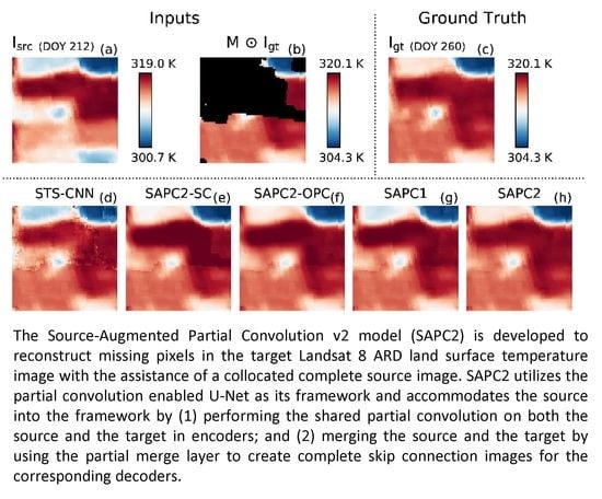
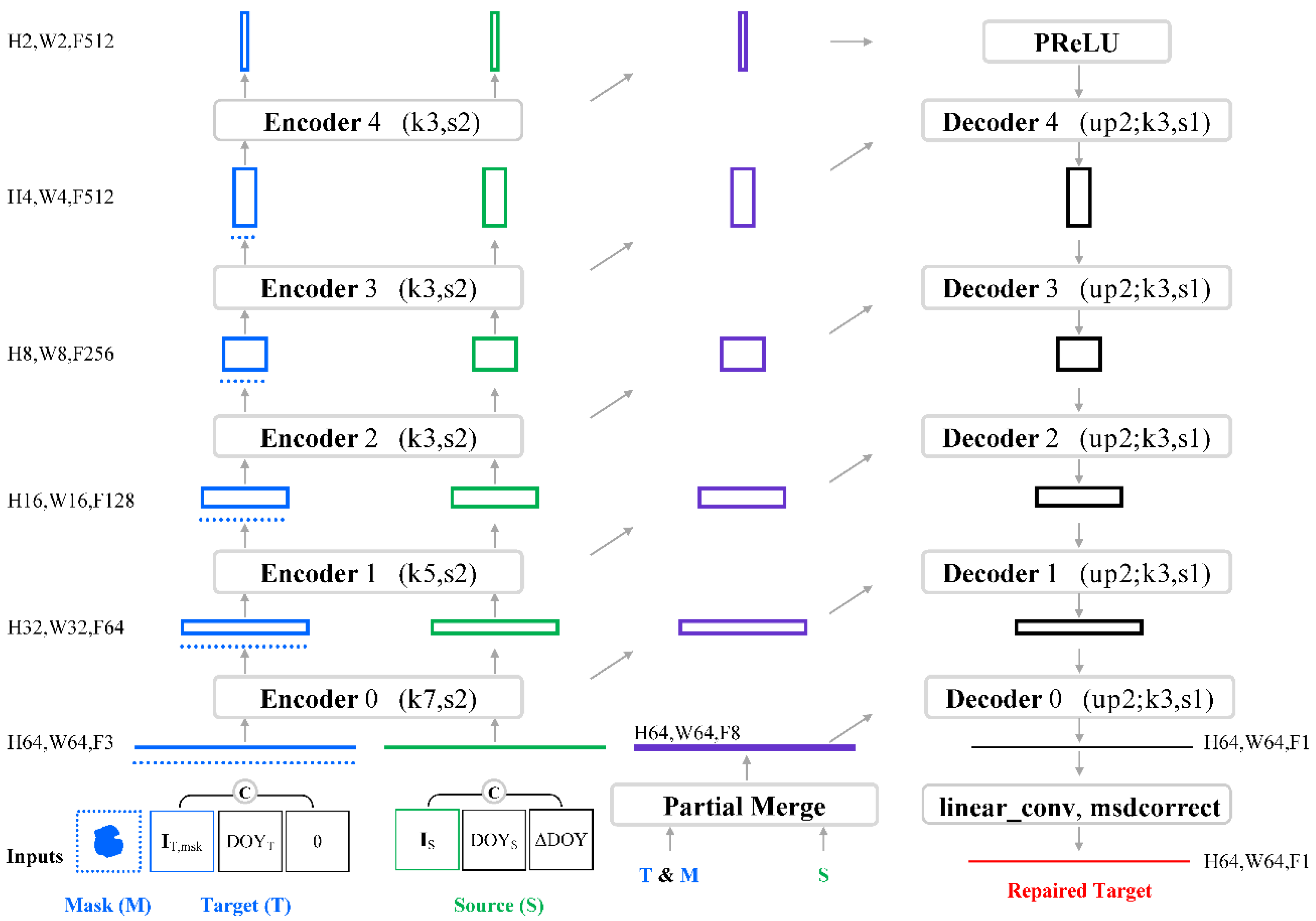
2.1.1. Overview

The goal of the proposed model is to reconstruct the missing pixels in a corrupted or masked LST image patch (the target), given a collocated complete image acquired on an adjacent date (the source), and the respective date information of both images. To achieve this goal, Chen et al. (2019) [33] proposed a Source-Augmented Partial Convolution neural network (hereafter SAPC1), which derives from the U-Net architecture and utilizes the partial convolution based operations to handle the missing pixels in the feature extraction and target-source merging process. This paper inherits the main design of SAPC1 but introduces a few modifications/improvements on the architecture, the training process, and the implementation.
Figure 1 gives an overview of the modified Source-Augmented Partial Convolution v2 (SAPC2) model. On the left bottom, SAPC2 receives a pair of input images: (1) the partially masked target image (T); and (2) the collocated complete source image (S). Each contains an LST image patch with the shape of 64 × 64 pixels, its acquisition date of year, and the date difference from the target image’s acquisition date. In addition, the target image contains a mask image indicating the unmasked and masked regions. SAPC2 first merges the input images into a complete 8-feature 64 × 64 image using the Partial Merge layer (see mid-bottom part in Figure 1). This image is reserved as the skip connection to provide details at the original spatial resolution for the last decoder. SAPC2 then passes the pair of target and source images through five stacked encoders to: (1) extract shared higher-level features from the target and source paths while reducing their spatial resolutions; (2) gradually diffuse information from the unmasked into the masked regions for the target path; and (3) reserve details along the spatial resolution hierarchy for the decoding phase. Specifically, each encoder will halve the spatial dimension (i.e., by using a constant stride of 2 in its convolutions) and double the features (until number of features reaches 512, plateauing afterwards). Following the original partial convolution design [32], the first two encoders have a slightly larger convolution kernel (i.e., 7 × 7 and 5 × 5) than the rest in order to capture and diffuse low-level features faster. Same as SAPC2′s first merging operation, each encoder also merges its output from the two paths into a complete image (skip connections, purple blocks in the middle of Figure 1) to facilitate the recovery of details in the corresponding decoder. At the end of the stacked encoders, it is guaranteed that the generated image (shape of 2 × 2) is free of missing values for any partially masked target images with the shape of 64 × 64. This image serves as the input image for the decoding path (on the right of Figure 1). SAPC2′s decoding path comprises five staked decoders and two additional linear layers. By merging the skip connections, the decoders reverse the process of encoders and gradually increase the spatial resolution until reaching the model input image’s spatial dimension. Additional linear transformations are applied to the last decoder’s output to generate the raw repaired target image (i.e., before replacing the unmasked part with true values). All nonlinear activation functions in SAPC2 are PReLU.

2.1.2. Encoder

To fulfill the three goals of the stacked encoders mentioned in the previous section (Section 2.1.1), each encoder shares the same structure, as depicted in Figure 2. The target and source images are either the model inputs or the outputs of the previous encoder layer. They are both passed through the same series of operators (with the shared weights) including a stride-2 partial convolution layer (described in Section 2.1.4), a batch normalization layer, and a Parametric Rectified Linear Unit (PReLU) activation to extract shared higher-level features. The partial convolution also fills in missing pixels around the boundaries of the mask with the convolution’s kernel size determining how far into the mask the filling can occur. To reduce the effects of the target’s missing pixels on estimating its true mean and standard deviation values, the masked part of the target image is temporarily set to random values with their mean and standard deviation matching the unmasked part before batch normalization. After PReLU activation, the processed target and source images are reported as two outputs for the next-level encoder. In addition, they are passed through a Partial Merge layer (described in Section 2.1.5) and another batch normalization layer to generate the complete image (i.e., the purple “M” box in Figure 2) that contains the merged target-source details at the current spatial resolution. This image, also called a skip connection, is also an output of the encoder and is reserved to be merged in the matching decoder.

2.1.3. Decoder

As a building block in the decoding path, each decoder (Figure 3) increases the spatial resolution of the main input image by a factor of two with the ancillary high-resolution details from a skip connection reserved by the matching encoder. The main input image is either from the final encoder or from the previous decoder output. The decoder first doubles its resolution with a non-parametric bilinear up-sampling operator. Then, it merges the upsampled with the skip connection from the matching encoder to improve the details. Section 2.1.5 describes the details of a Merge layer. Note that all images involved in the decoder are free of missing pixels, therefore the Partial Merge layer is not needed. Finally, the decoder passes the merged output through a standard batch normalization layer and a PReLU activation to generate the layer’s output.

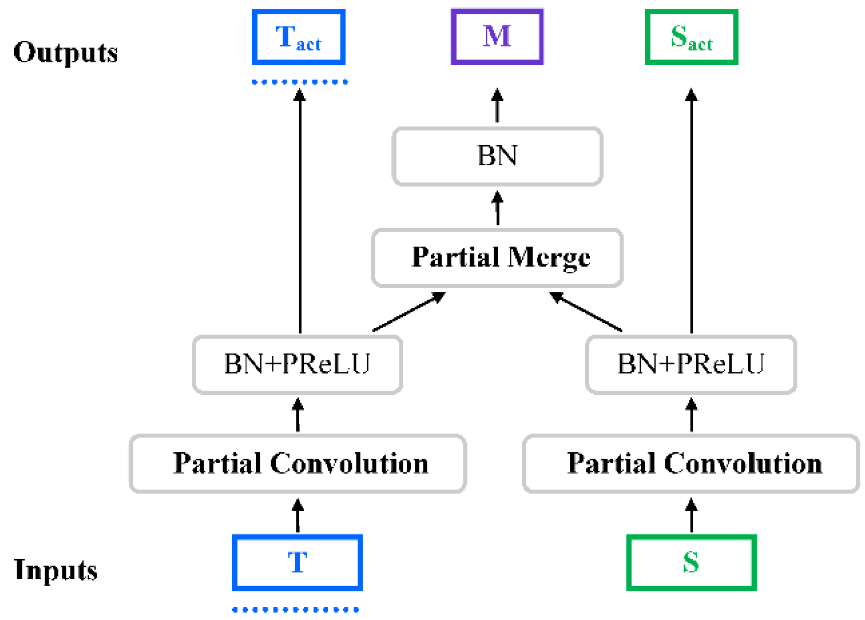
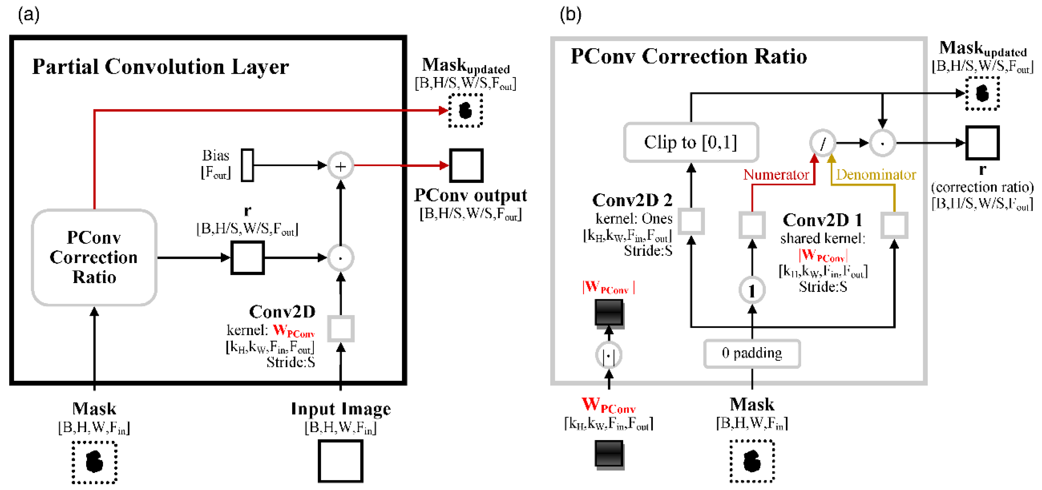
2.1.4. Partial Convolution Layer

A Partial Convolution layer (PConv), first proposed by Liu et al. (2018) [32] and modified by Chen et al. (2019) [33], is the extension of the standard 2D convolution on scenarios where input image may contain missing values. In each sliding window of convolution, PConv first conducts the standard 2D convolution and then corrects the effects of missing pixels by multiplying the convolution result with a ratio of some metric for the whole image and that for the unmasked part. As for the metric, Liu et al. (2018) [32] selected the count of pixels while Chen et al. (2019) [33] used the sum of absolute convolution weights. Note that if the correction coefficient is a constant value 1, PConv becomes a standard convolution. In addition, PConv provides the updated mask that is associated with the convolution result. The core PConv operations in a sliding window of convolution for creating one (e.g., jth) output feature are expressed in the following equations:
x j = { sum ( W j ( X M ) ) r a t i o j p c o n v + b j , sum ( M ) > 0 0 , o t h e r w i s e
m j = m = { 1 , sum ( M ) > 0 0 , o t h e r w i s e
where SAPC2 and SAPC1 both define the correction ratio as:
r a t i o j p c o n v = sum ( | W j | 1 ) sum ( | W j | M )
X and M denote the input image and mask slices in the sliding window. Wj and bj are the convolution weights and bias (for the jth output feature). xj’ and mj’ are the PConv’s (jth) output value and the corresponding updated mask value. Figure 4 gives the flowchart of the PConv layer in SAPC2.

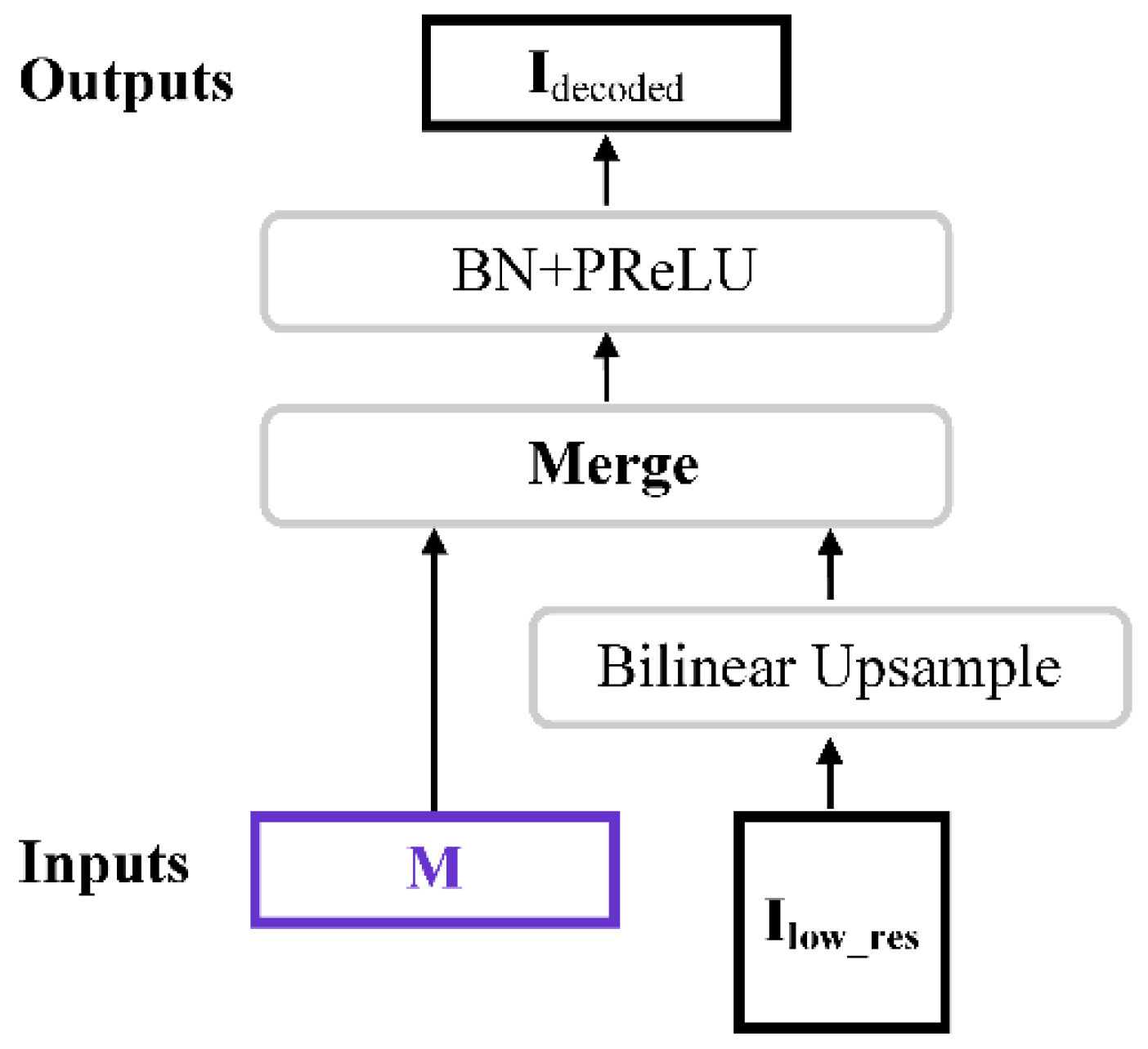
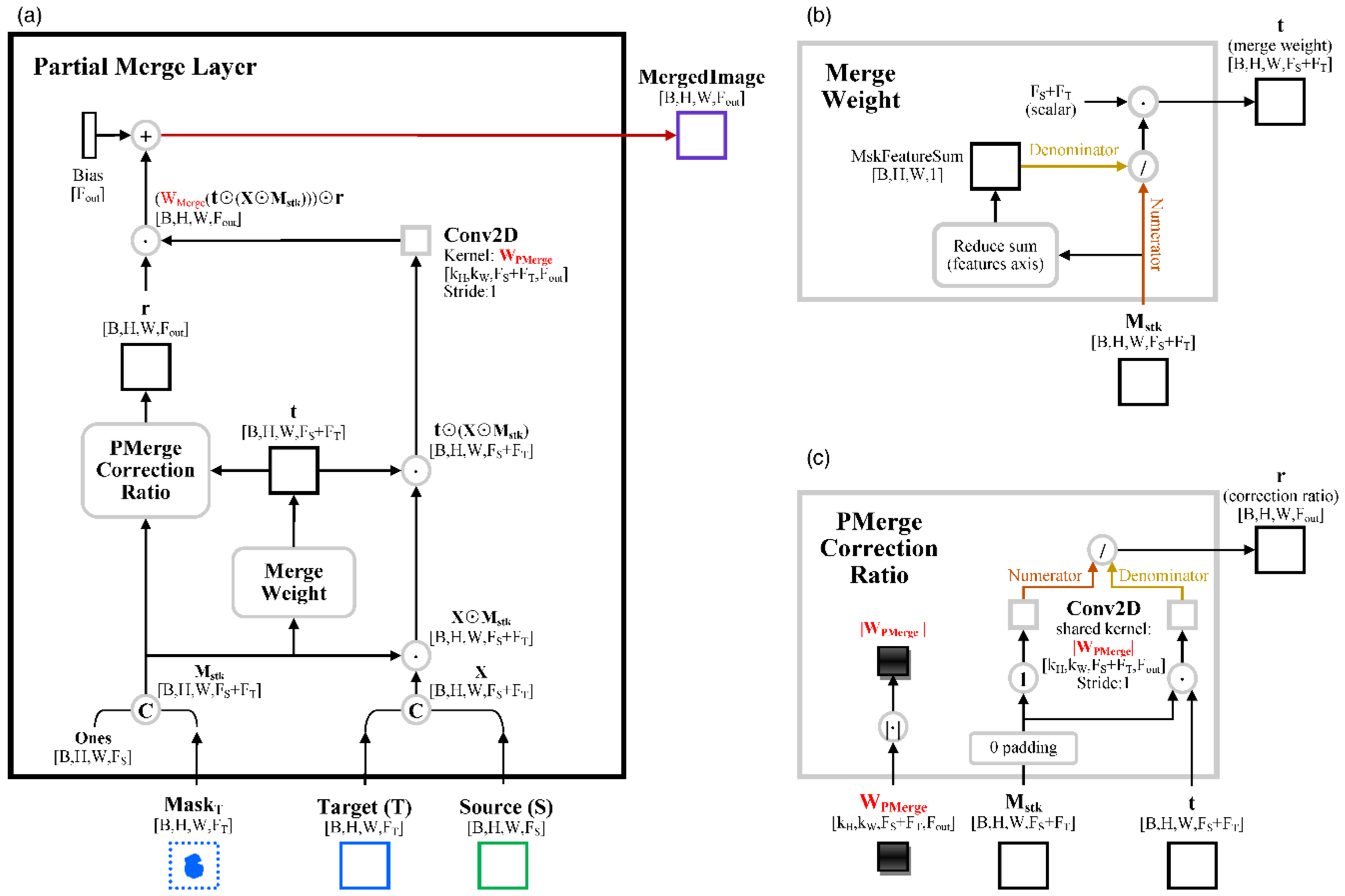
2.1.5. Partial Merge Layer and Merge Layer

The Partial Merge layer (PMerge) takes a partially-masked target image (along with its mask image) and the corresponding complete source image as inputs, merges them into a complete same-spatial-dimensions image using a modified partial convolution operation. PMerge first stack the target and source images along the feature dimension to create the stacked image. Similarly, it stacks target’s mask and source’s mask (an all-one image with the same shape of the source image) to create the stacked mask. The reason PConv is not chosen to merge the stacked image is that the PConv result may have inconsistent mean and variation between the target-source-both-unmasked region and the target-masked-but-source-unmasked region. For example, if both the source and true target are a one-feature image with a constant value 0.1, and the PConv kernel is of shape [1,1,2,1] and has a constant value of 0.5, the PConv result at a target-unmasked pixel is 0.1 (=0.5 ∗ 0.1 + 0.5 ∗ 0.1), which is twice as large as at a target-masked pixel (i.e., 0.05 (=0.5 ∗ 0.1 + 0.5 ∗ 0.0)). To overcome this issue, Chen et al. (2019) [33] introduced a feature-dimension weighting mechanism in PConv to ensure that the equivalent number of non-masked values participating the convolution at each pixel remains the same between the two regions. The modified PConv is the called PMerge. Formally, a PMerge operation in a sliding window of convolution for creating one (e.g., jth) output feature is expressed by the following equations:
x j = sum ( W j ( X M t M ) ) r a t i o j p m e r g e + b j
where the feature-dimension weighting mechanism is implemented by multiplying the mask M with the merge weight t M in Equation (4) and t M is defined by
t M = t ( M ) = M / f F M f
where F denotes the entire feature layers. Since t M is part of the convolution, the correction ratio for PMerge also includes t M :
r a t i o j p m e r g e = sum ( | W j | ( t 1 1 ) ) sum ( | W j | ( t M M ) )
t 1 is obtained by Equation (5) with an all-one array with the same shape of M. Other notations in Equations (4)–(6) are the same as in PConv. Figure 5 presents the flowchart of the PMerge layer.
The Merge layer (Merge), which is used to combine the upsampled image with the matching skip connection in decoders, is a simplified version of PMerge. Since both input images of Merge are complete, the term t M will be equal to t 1 and can be removed from Equations (4)–(6). However, Merge cannot be replaced with a standard convolution because the padded image boundary will have the value 0 (i.e., the correction of convolution in the padding regions is still needed). There are two differences between Merge and PConv: (1) Merge has two inputs while PConv only has one; and (2) Merge output is always complete and therefore does not need the mask update step. A Merge operation is expressed by the following equations:
x j = sum ( W j ( X M ) ) r a t i o j m e r g e + b j
r a t i o j m e r g e = sum ( | W j | 1 ) sum ( | W j | M )
All notations in Equations (7) and (8) are the same as in PConv. Figure 6 presents the flowchart of the Merge layer.

2.1.6. Linear Convolution Layer and Final Mean and Standard Deviation Adjustment Layer

These two layers perform additional linear transformations on top of the stacked decoders for fine adjustment on model prediction. The Linear Convolution layer takes the output of the last decoder as input and performs a standard 2D convolution with kernel size 1 × 1 to scale the distribution of the decoder output. It is a global operation, which affects all samples the same way. In contrast, the final layer is a non-parametric local operation, which affects each sample independently. The final layer linearly adjusts the mean and standard deviation of the entire Linear Convolution output for each sample so that the mean and standard deviation of the Linear Convolution output match those of the model target input in the unmasked region (based on the model mask input). The output of the final layer is a raw prediction, which is mosaicked with the unmasked part of the model target input to generate the mosaic prediction.

2.2. Baseline Models

In this paper, in addition to the proposed model (SAPC2), three other source-augmentation partial convolution based models (i.e., SAPC1, SAPC2-OPC, and SAPC2-SC) as well as the unified spatial-temporal-spectral convolution neural network (STS-CNN) are implemented as baseline models. This study focuses on performance difference induced by the model architecture and tries to minimize influence from other aspects. Therefore, when possible, all baseline models share the same data pipeline, training environment, loss and metric functions, etc. as the proposed model (i.e., SAPC2).

2.2.1. SAPC1

The main differences of SAPC1′s [33] architecture compared with SAPC2 include:
(a)
the initial skip connection for the last decoder is the source image instead of PMerge of the source and target;
(b)
the first encoder does not have batch normalization after PConv;
(c)
the first four encoders’ PConv s use ReLU as activations;
(d)
the last (5th) encoder is implemented as PConv on the previous encoder’s target output image and there is no batch normalization or activation before passing its output to the first decoder;
(e)
the first four decoders’ (i.e., Decoders 4, 3, 2, and 1 in Figure 1) activations are LeakyReLU;
(f)
the last decoder does not have batch normalization nor activation; and
(g)
no unmasked mean square error (MSE) losses imposed between the encoder and decoder pairs (e.g., encoder 1′s target input vs. decoder 1′s output) to encourage the matching levels have similar abstract features.

2.2.2. SAPC2-Original Partial Convolution (SAPC2-OPC)

SAPC2-OPC refers to the baseline model that does not include absolute weights in the correction ratio calculation (i.e., Equations (3), (6) and (8)) for all PConv, PMerge, and Merge layers. Other than these differences, SAPC2-OPC is the same as SAPC2.

2.2.3. SAPC2-Standard Convolution (SAPC2-SC)

SAPC2-SC refers to the baseline model that sets a constant value 1 to the correction ratios (Equations (3), (6) and (8)) for all PConv, PMerge, and Merge layers. Other than these differences, SAPC2-SC is the same as SAPC2.

2.2.4. STS-CNN

The STS-CNN has a significantly different architecture (see details in Figure 3 of [31]) from SAPC2. Here is an incomplete list highlighting some prominent ones
(a)
There is almost no change in number of features (i.e., 60) across the STS-CNN framework except in the first and last convolution steps. The spatial size is constant for the entire network. In contrast, SAPC2 is based on U-Net framework with intended feature and spatial size variations.
(b)
STS-CNN utilizes multiscale convolution to extract more features for the multi-context information and dilated convolution to enlarge the receptive field while maintaining the minimal kernel size.
(c)
STS-CNN uses standard convolution instead of partial convolution in the framework.
(d)
STS-CNN uses ReLU for all activations.
In addition to the architecture, some modifications on the data pipeline and loss/metric functions are made.
(e)
STS-CNN takes the satellite images as inputs but does not utilize date related inputs as in SAPC2 (i.e., day of year and date difference from the target acquisition date). To take into account the seasonal LST variations, each sample’s source and target images are independently scaled to the same range [0,1].
(f)
STS-CNN aims to have fast convergence and chooses to optimize the MSE of the residual map, which is close to (but not the same as) the masked MSE used in SAPC2. As a result, many metric/loss functions for SAPC2 that are dependent on the unmasked part or on the feature domains are not provided.

2.3. Training Procedure

2.3.1. Number of Trainable Variables

The SAPC2, SAPC2-OPC, and SAPC2-SC models have the same number of trainable variables: 2,761,446. The SAPC1 has fewer trainable variables: 1,969,204. The STS-CNN has the fewest trainable variables: 296,161.

2.3.2. Loss Functions

SAPC2 inherits the four losses/metrics defined in Chen et al. (2019) [33], including two MSEs on the raw repaired image
L unmasked = M S E unmasked = M ( I out I gt ) 2 2 M ,  
L masked = M S E masked = ( 1 M ) ( I out I gt ) 2 2 ( 1 M )
and two MSEs on the Sobel filtered raw repaired image
L sobel , unmasked = M S E sobel , unmasked = M ( S o b e l ( I out ) S o b e l ( I gt ) ) 2 2 2 M
L Sobel , masked = M S E sobel , masked | C C ( I S , I gt ) | = ( 1 M ) ( S o b e l ( I out ) S o b e l ( I gt ) ) 2 2 2 ( 1 M ) | C C ( I S , I gt ) |
where Iout is the raw model prediction (i.e., before replacing the unmasked part with the target image). Igt is the ground truth (i.e., complete target image). M is the mask in which value 1 indicates unmasked (good) pixels and value 0 indicates masked pixels. CC() is the correlation coefficient function. Sobel() is the function that returns the two (i.e., horizontal and vertical) Sobel edge maps.
SAPC2 introduces additional loss terms (with their sum denoted by Lrecovery) that measure the MSEs between the encoders’ target inputs and the corresponding decoders’ outputs in the unmasked regions to encourage the recovery of similar features at the matching encoder–decoder levels. These loss terms do not include the Encoder 1–Decoder 1 level.
In addition, all trainable variables (including convolution weights, PReLU alphas, etc.) are subject to the l2 regularization loss Lreg,l2.
For training the model, the total loss function is defined as the weighted sum of the six losses abovementioned:
L total = 1.0 L unmasked + 2.15 L masked + 0.4 L sobel , unmasked + 0.86 L sobel , masked + 0.01 L recovery + 3.51 e 7 L reg , l 2
The weights of these losses are determined by hyperparameter searching.

2.3.3. Learning Rate Scheduling

Smith (2017) [34] proposed several cyclical learning rate scheduling methods for deep neural networks. The main difference of these methods compared with the monotonically decreasing learning rate is to vary the learning rate cyclically between reasonable boundary values. All of these methods have a fixed minimum learning rate and an initial learning rate range that is attenuated with training steps or epochs. The actual learning rate will linearly cycle within the range defined by [minimum rate, minimum rate + instant range]. For example, the exponential cyclical scheduling uses a power function to describe the attenuation process: attenuation_fn(cycle) = gamma ** cycle, where gamma is a constant (e.g., 0.96) and cycle is the current step’s epoch (with fraction, starting from 1.0).
A new scheduling method (exponential cyclical scheduling v2) is derived, inspired by the exponential cyclical scheduling with the key change in allowing the minimum learning rate to decay at the same rate as the maximum learning rate. The first step the new method is to determine the ratio (rnep) between the initial minimum learning rate (lrmin,init) and the final minimum learning rate (lrmin,nep) at a given epochs (nep). With these two parameters, and assuming a constant decay rate between any two adjacent epochs, the decay rate per epoch (dep) is expressed by the following equation:
d ep = r nep 1 n ep 1
and the maximum (lrmax,iep) and minimum (lrmin,iep) learning rates and their range (lrrange,iep) at the ith epoch (iep) are expressed by:
l r max , iep = l r max , init ( d ep ) iep
l r min , iep = l r min , init ( d ep ) iep
l r range , iep = l r max , iep l r min , iep
where lrmax,init is the initial maximum learning rate. For the DNN in this study, it was found that lrmax,init three times larger than lrmin,init showed the best model performance.
With lrmin,iep and lrrange,iep, the remaining steps to derive the per step learning rate is the same as other cyclical scheduling methods. For a step p within the epoch iep, the learning rate at p (lrp,iep) is derived from the following equations:
c y c l e = floor ( 1 + p / ( 2 s t e p s i z e ) ) x = abs ( p / s t e p s i z e 2 c y c l e + 1 ) l r p , iep = l r min , iep + l r range , iep max ( 0 , 1 x )
where stepsize is the number of steps for half of the period or cycle length [34].

2.4. Implementation

2.4.1. Software and Hardware

The SAPC2 model is implemented using TensorFlow (tf [35]) v2.2. All main layers such as PConv, PMerge, Merge, Encoder, Decoder, and all lambda layers (e.g., for copy and slice tensors) are implemented as subclasses of the keras base Layer (tf.keras.layers.Layer). The total loss function is implemented as subclass of tf.keras.losses.Loss. The training utilities are implemented as subclasses of tf.keras.callbacks.Callback. To reduce the retracing time, metric functions, standalone functions, as well as some custom layers’ member functions that contain heavy tf operations, are decorated by the tf.function wrapper. The entire architecture building upon the custom layers is assembled using the keras functional model API (tf.keras.Model). A Python interface function is created to manage the entire training process including the data pipeline preparation, the keras model creation, compilation, and fitting, and the results logging. Important hyperparameters are passed to the interface function through command line arguments. The implementation of the four baseline models is similar to SAPC2 with the main differences in the underlying architectures.
The models are trained on Google Cloud Platform (GCP) Cloud TPU each for 20 epochs. To be consistent across models, the virtual machine (VM) for training is fixed to be an n1-standard-8 VM plus a v3-8 tpu in the us-central1 region. This setting allows a batch size of 2048, lrmax,init of 7.05 × 10⁻⁴, and lrmin,init of 2.35 × 10⁻⁴ for all five models.
The analysis of the optimized models was conducted on a desktop with an Intel Xeon E5-2630 v3 CPU, 32 GB of RAM, and a NVIDIA GeFore GTX 1080 Ti GPU.

2.4.2. Hyperparameter Tuning

Eight hyperparameters, including the minimum and maximum initial learning rates (lrmin,init and lrmax,init) and the weights for the six loss terms in Equation(13), are tuned using the grid search with approximately 21% of the full training dataset. Since the weights for the total loss may not be available at the time of hyperparameter tuning, the objective function for tuning is the average of masked and unmasked MSE.

2.5. Dataset

The pairs of target-source LST image/mask patches used in this study originate from the Landsat 8 Analysis Ready Data (ARD) Land Surface Temperature product [5], which is distributed through the EarthExplorer website (https://earthexplorer.usgs.gov/). The original ARD LST tiles (with cloud cover and shadow both less than 80%) in the Colorado region for 2014–2018 were combined in Google Earth Engine (https://earthengine.google.com/). Their Quality Assessment (QA) information was used to create the mask maps distinguishing the bad/missing pixels (e.g., caused by cloud or outside the boundary of a satellite scene) from the good pixels (containing valid LST values). On two nearby days (i.e., absolute acquisition dates difference less than 48 days), pairs of 65 × 65 all-good-pixels LST patches (along with their day-of-year (DOY) and DOY difference from each other) were randomly sampled to create the initial LST pairs. These initial pairs were cropped to 64 × 64 pixels. Each pair’s two images were assigned with either the source or ground truth roles. Then, the size of the pairs was doubled by flipping the assigned roles. The feature “DOY difference from each other” was converted to “DOY difference from the target acquisition date” by setting this feature for the target to value zero. Next, each of them was paired with one same-size mask randomly sampled from the mask maps, creating the target image by multiplying the ground truth with the mask. Note that the mask here defines the good pixels (unmasked) with value one and the bad pixels (masked) with value zero. The expanded pairs were further augmented (e.g., through flips, rotations, and their combinations), standardized (i.e., normalized by individual features except for the mask), and sharded (i.e., randomly distribute samples into 1000 files) on the Google Cloud Platform (GCP) DataFlow platform. Since the SAPC2 model relies on the source image to supplement information in the masked regions, only samples with highly correlated source-target pairs (i.e., correlation coefficient ≥ 0.8) were used. This procedure generates ~2.475 million data samples, 95% of which (~2.352 million samples) were used for training and the rest 5% (~0.124 million samples) were reserved for validation.

3. Results

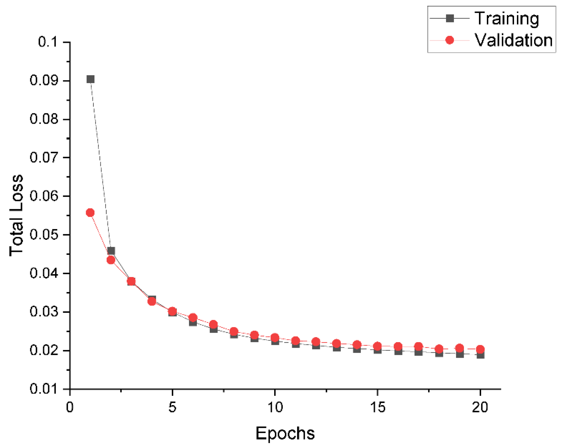
3.1. Training Process

Figure 7 shows the total losses vs. epochs for the SAPC2 model. With the new learning rate scheduling (i.e., exponential cyclical scheduling v2), the total losses of training and validation both decrease across the 20 epochs with slight fluctuations. No sign of overfitting is observed. Similar results are found for all four baseline models (data not shown).
With the batch size of 2048 and the v3-8 tpu accelerator, the average training time of SAPC2 over the 20 epochs is about 524 s per epoch. The first five epochs took slightly longer (534–547 s) than the rest (518–529 s). The average training time for SAPC1, SAPC2-OPC, SAPC2-SC, and STS-CNN are 461, 524, 463, and 449 s per epoch, respectively.

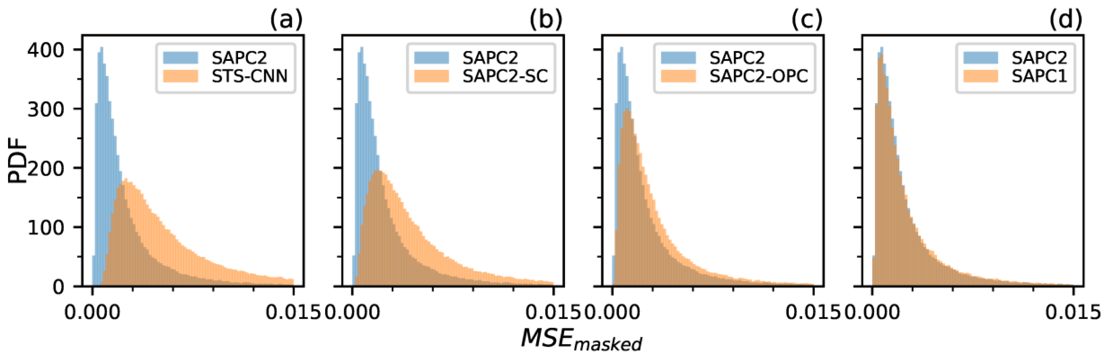
3.2. Validation Statistics

The model prediction refers to the raw model output (e.g., the bottom right red line (Repaired Target) in Figure 1), and the mosaicked model prediction replaces the unmasked part of the model prediction with that in the target image. For the four SAPC-based models, because their total loss for training relies on both the masked and unmasked parts, their model predictions in the unmasked part should have meaningful patterns that are close to the target and worth evaluation. However, for STS-CNN, because it optimizes residual map, its model prediction in the unmasked part is close to all zeros and should not be evaluated. Therefore, for STS-CNN, the evaluation of the model performance focuses on the mosaicked model prediction or on the masked part of the model prediction.
To compare the performances of the five models, nine metrics were calculated on each validation data sample:
  • MSEmasked: The Mean Square Error (MSE) between the model prediction and ground truth in the masked part
  • Lsobel,masked: The source-target-correlation-coefficient-weighted MSE between the Sobel-edge transformed model prediction and the corresponding transformed ground truth in the masked part
  • MSEunmasked: The MSE between the model prediction and ground truth in the unmasked part
  • MSEsobel,unmasked: The MSE between the Sobel-edge transformed model prediction and the corresponding transformed ground truth in the unmasked part
  • MSEweighted: The weighted sum of MSEmasked, Lsobel,masked, MSEunmasked, and MSEsobel,unmasked, with the weights given in Equation (13)
  • MSEmosaic: The MSE between the mosaicked model prediction and ground truth
  • CCmosaic: The Correlation Coefficient between the mosaicked model prediction and ground truth
  • PSNRmosaic: The Peak Signal-To-Noise ratio of the mosaicked model prediction
  • SSIMmosaic: The Structural Similarity Index of the mosaicked model prediction
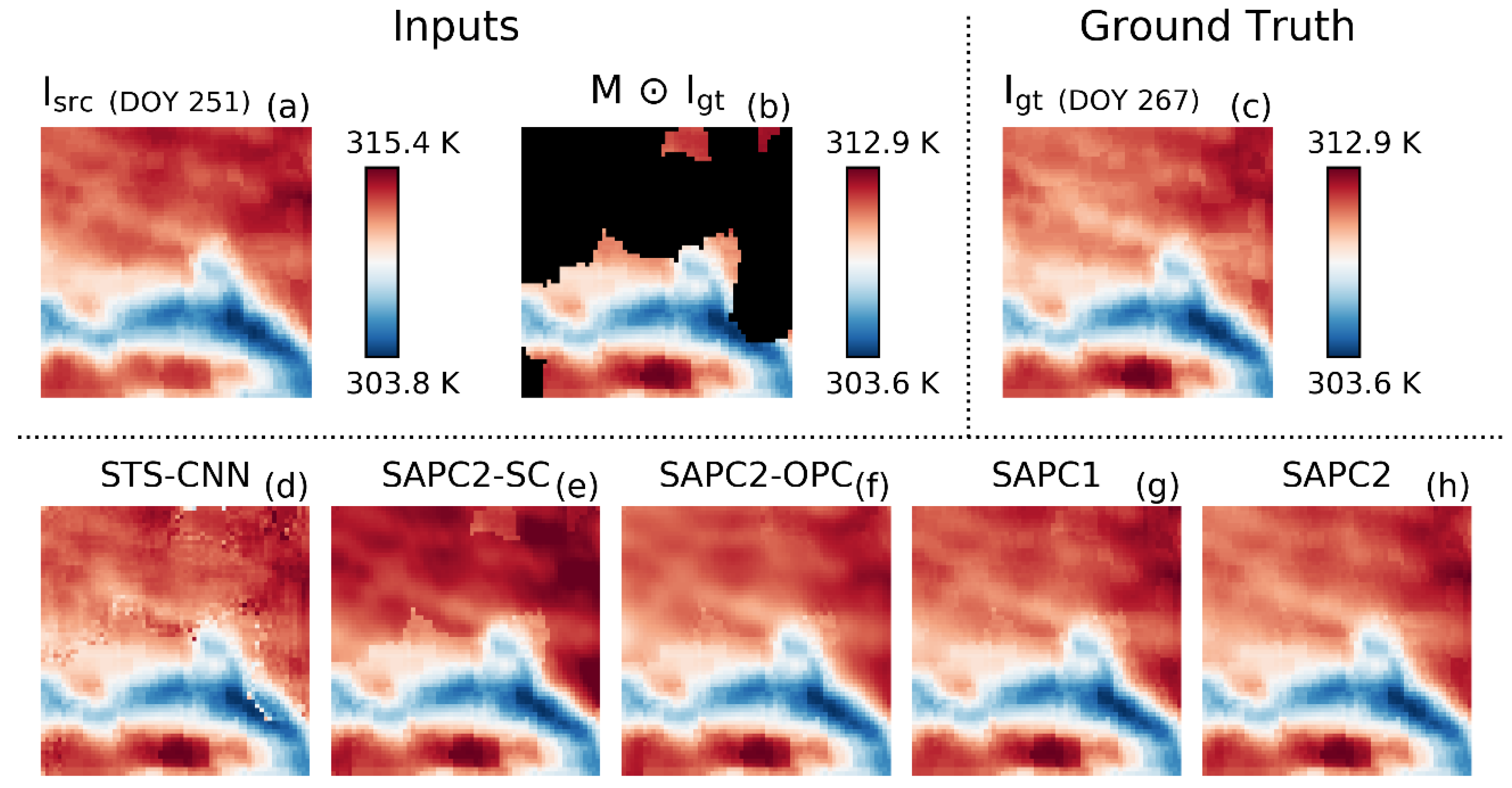
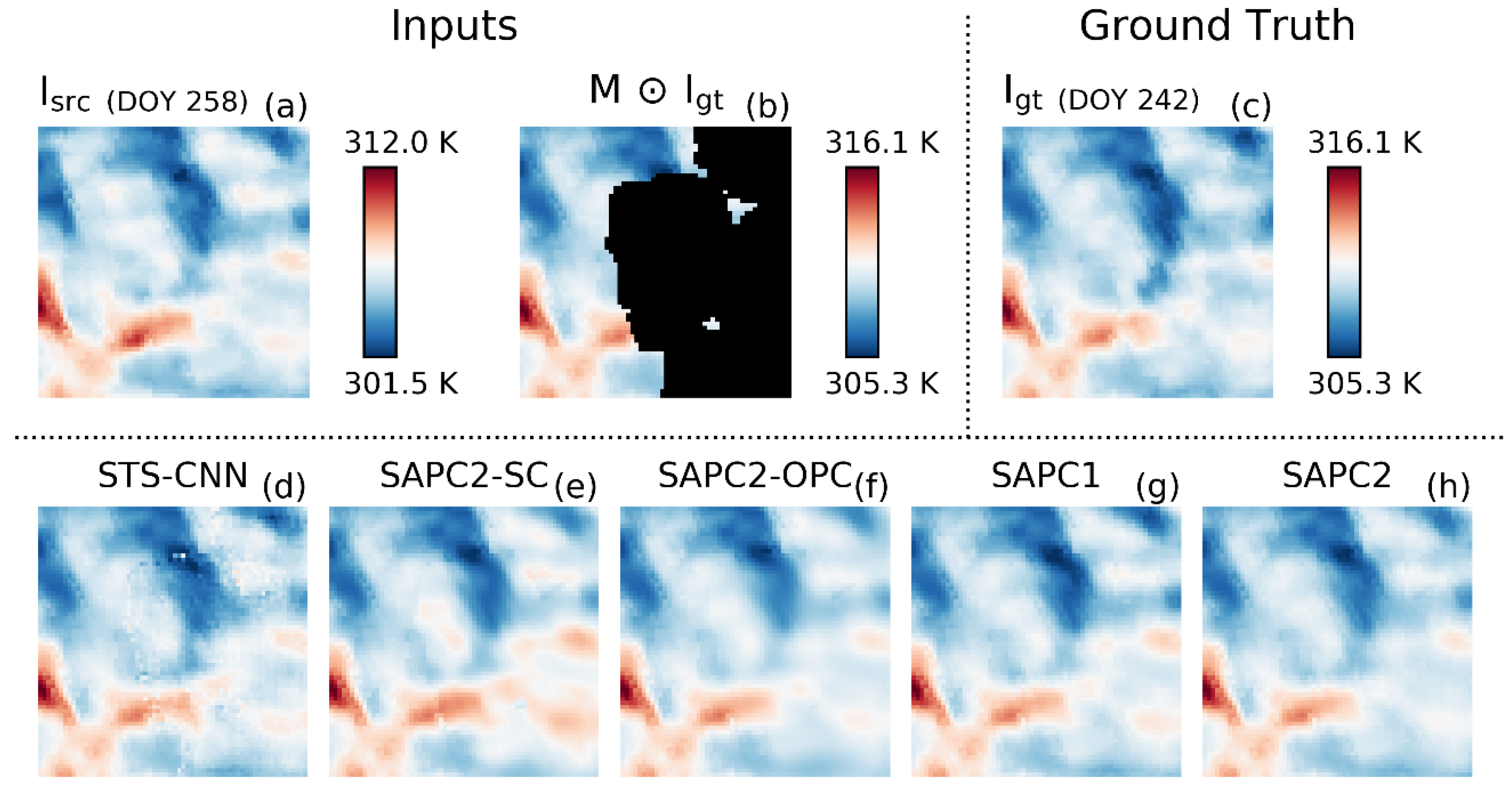
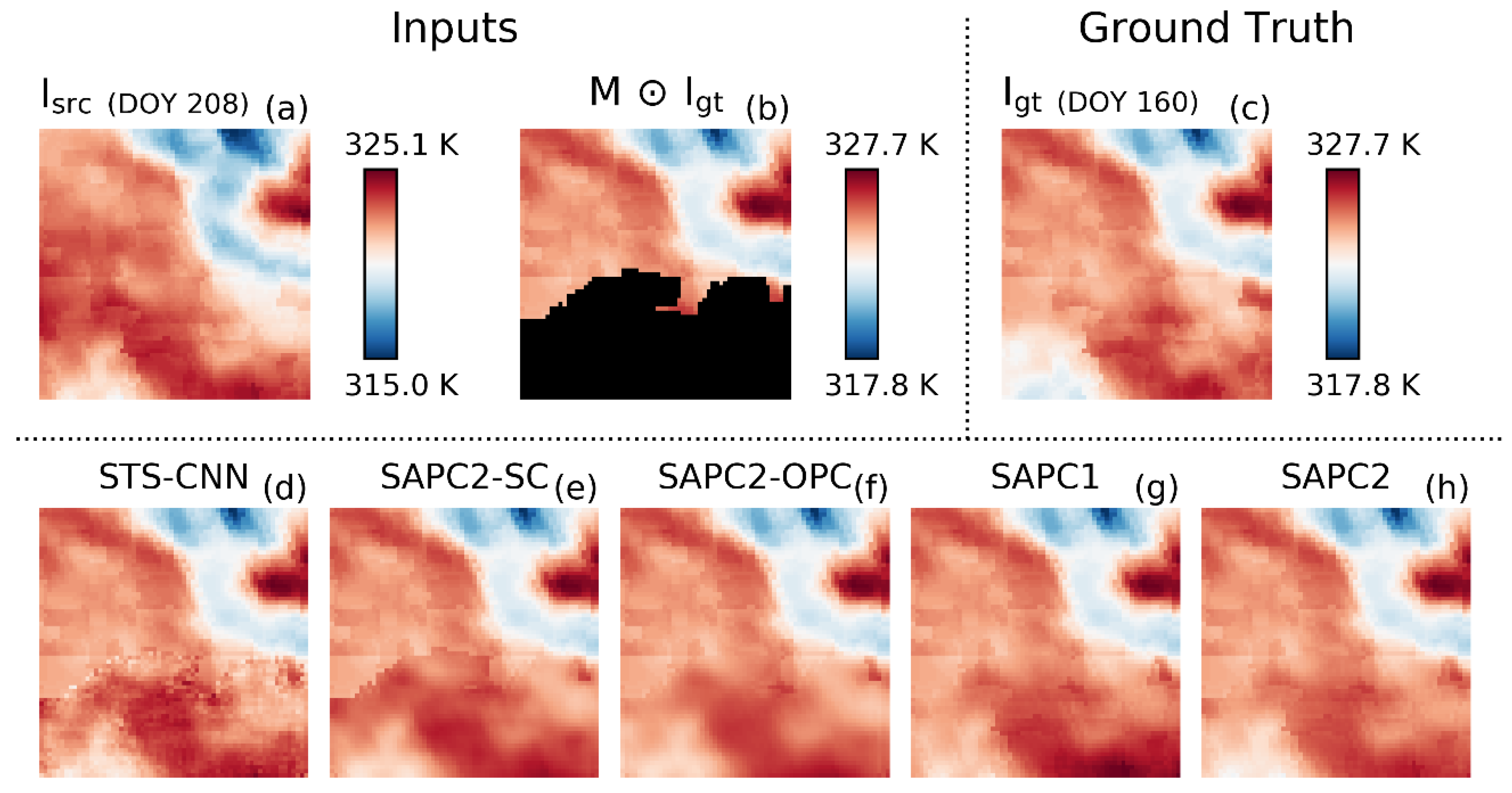
Table 1 lists the means and standard deviations of the nine metrics on the entire validation dataset (~0.124 million samples) for all five models. It is seen that the proposed model (SAPC2) has the lowest mean values on all six MSE metrics and the highest mean values on the other three metrics (i.e., CCmosaic, PSNRmosaic, and SSIMmosaic). SAPC2 also has the lowest standard deviation values on all metrics except for PSNRmosaic, on which STS-CNN has the lowest value (4.33).
One way to summarize the model performance based on the nine metrics is to assign a score for each model based on its order (best = 1 and worst = 5) in each metric and calculate the average value of the orders across the applicable metrics as the comprehensive score for each model. For the metrics’ means, the comprehensive score for SAPC2 is the highest (1), followed by SAPC1 (2), SAPC2-OPC (3.3), SAPC2-SC (3.7), and STS-CNN (5). For the metrics’ standard deviations, the comprehensive score for SPAC2 is also the highest (1.3), followed by SAPC1 (2.3), SAPC2-OPC (3.2), SAPC2-SC (3.6), and STS-CNN (4.2). The comprehensive scores derived from means and standard deviations both suggest that SAPC2 has the best performance, followed by SAPC1, SAPC2-OPC, SAPC2-SC, and STS-CNN.
To have a deeper insight on the model performance, Probability Density Functions (PDFs) of the nine metrics over the entire validation dataset are analyzed. Figure 8 compares the PDFs between SAPC2 and the other four baseline models on the metric MSEmasked. The SAPC2’s PDFs are displayed as the blue shapes in the four subplots, while the orange shapes represent the four baselines’ PDFs. It is seen that the STS-CNN has the most distinguishable PDF than SAPC2 (Figure 8a). The SAPC2’s left end is closer to zero, its peak is higher and has a smaller MSE value, and its right tail is much shorter than STS-CNN. Although the similar patterns are also seen on SAPC2-SC (Figure 8b), and SAPC2-OPC (Figure 8c), their PDFs are closer to matching SAPC2’s. The PDF of SAPC1 (Figure 8d) is almost identical to that of SAPC2, but from the left end to MSEmasked ~= 0.025, SAPC2 (the blue bars) has slightly higher PDF values. All other metrics’ PDF comparison shows similar distinguishable results (data not shown).

3.3. Case Study

Figure 9, Figure 10, Figure 11, Figure 12, Figure 13 and Figure 14 show the five models’ mosaicked prediction results on six cases.
Figure 9 shows a case with a pair of source-target inputs that are acquired 48 days apart. Even though the source and the ground truth are highly correlated (i.e., correlation coefficient, cc = 0.957), an 8.3 K difference in maximum temperature but only 2.4 K difference in minimum temperature and a close-to-half masked fraction make it an interesting case. Overall, the SAPC2 (h) has the lowest MSEmasked and Lsobel,masked values among the five models (i.e., 0.00183 and 0.00268). They are 67% and 46% lower than those of SAPC1 (0.00560 and 0.00494), 55% and 32% lower than those of SAPC2-OPC (0.00403 and 0.00394), 83% and 59% lower than those of SAPC2-SC (0.01070 and 0.00647), and 59% and 98% lower than those of STS-CNN (0.00449 and 0.13682). According to these metrics, SAPC2 is the best model for the case. Along the left edge of the mask, Figure 9d–g shows some significant edge artifacts, where STS-CNN exhibits some random noisy pixels and the three SAPC-based models show smooth pattern but abrupt color shift near the edge area. The details in the masked regions are not well recovered by all methods due to the source image’s quality; however, the overall color scale of SAPC2 in the masked part is closer to the ground truth than the other methods.
Case 2 (Figure 10) has a more adjacently acquired source image (only 16 days away from the target). The quality of the source is also better than the first case. Not only cc between the source and the ground truth is slightly higher (0.975 vs. 0.957), but the micro patterns including sharp boundaries match better. As a result, SAPC2 is capable of restoring both the color scale and details from the source without displaying striking edge effects. In contrast, all other methods exhibit some levels of visible edge effects. In terms of metrics, SAPC2 also shows the best performance. The values of MSEmasked and Lsobel,masked for SPAC2 are 0.00075 and 0.00267, respectively. They are 53% and 14% lower than those of SPAC1 (0.00161 and 0.00312), 44% and 32% lower than those of SPAC2-OPC (0.00134 and 0.00392), 91% and 65% lower than those of SPAC2-SC (0.00843 and 0.00761), and 67% and 98% lower than those of STS-CNN (0.00227 and 0.11243). According to these metrics, SAPC2 is the best model for Case 2.
Case 3 (Figure 11) has a similar temperature range between the source and the ground truth even though they are acquired 48 days apart. Figure 11d–g (i.e., STS-CNN, SAPC2-SC, SAPC2-OPC, and SAPC1) shows various levels of artifacts near the bottom of the top mask edge while subplot Figure 11h (SAPC2) does not show any visible edge effects. Inside the top mask region, STS-CNN demonstrates some noisy pixels while SAPC2-SC and SAPC2-OPC lose the details and show blurry results. SAPC1 reserves some sharper details but its color scale is slightly off the ground truth. In terms of metrics, the values of MSEmasked and Lsobel,masked for SPAC2 are 0.00126 and 0.00917, respectively. They are 39% and 16% lower than those of SPAC1 (0.00207 and 0.01098), 40% and 13% lower than those of SPAC2-OPC (0.00211 and 0.01057), 75% and 23% lower than those of SPAC2-SC (0.00508 and 0.01194), and 69% and 86% lower than those of STS-CNN (0.00410 and 0.06764). According to these metrics, SAPC2 is the best model for Case 3.
In Case 4 (Figure 12), all methods restore the dark-blue block with sharp edges at the center of the ground truth with some lighter-blue and dilated shape due to the discrepancy between the source and the ground truth in the region. However, at the bottom right corner, SAPC2 recovers the whitish block closer to the ground truth than other methods. SAPC2-SC and SAPC2-OPC show blurry patterns in the masked region. STS-CNN’s result is noisy near the boundaries of the mask. In terms of metrics, the values of MSEmasked and Lsobel,masked for SPAC2 are 0.00106 and 0.00657, respectively. They are 36% and 9% lower than those of SPAC1 (0.00166 and 0.00722), 55% and 20% lower than those of SPAC2-OPC (0.00236 and 0.00824), 80% and 30% lower than those of SPAC2-SC (0.00528 and 0.00941), and 43% and 83% lower than those of STS-CNN (0.00187 and 0.03858). According to these metrics, SAPC2 is the best model for Case 4.
Case 5 (Figure 13) has a slightly lower cc (i.e., 0.915) between the source and the ground truth. The edge effects appear in all methods’ mosaicked predictions but are least evident in SAPC2′s. For example, there is one unmasked pixel on the left of the mask. Other than SAPC2, all methods show a darker-than-surrounding pixel in their predictions. In addition, SAPC2 recovers the color scale in most masked region closer to the ground truth. For example, on the top left of the mask, even though the source shows light blue pattern, SAPC2 correctly fill that region with light red color. In the middle of the mask where SAPC2-SC restores a dark red “Z”-shaped block, SAPC2-SC, SAPC2-OPC, and SAPC1 all fill it with darker colors than the ground truth while SAPC2′s color scale in the region looks closer to the ground truth. As in previous cases, STS-CNN exhibits strong noise near the mask’s edge. In terms of metrics, the values of MSEmasked and Lsobel,masked for SPAC2 are 0.00277 and 0.01194, respectively. They are 68% and 49% lower than those of SPAC1 (0.00872 and 0.02335), 39% and 21% lower than those of SPAC2-OPC (0.00457 and 0.01516), 65% and 31% lower than those of SPAC2-SC (0.00787 and 0.01729), and 85% and 96% lower than those of STS-CNN (0.01866 and 0.31452). According to these metrics, SAPC2 is the best model for Case 5.
Case 6 (Figure 14) has the lowest cc (i.e., 0.839) between the source and the ground truth among the six presented cases. STS-CNN’s prediction is noisy across the entire masked region. Both SAPC2-SC and SAPC2-OPC show blurry result with some clear edge effects. SAPC1′s result recovers most details but the color scale in the masked region (especially near the bottom line) is slight off from the ground truth. In terms of metrics, the values of MSEmasked and Lsobel,masked for SPAC2 are 0.00233 and 0.00536, respectively. They are 53% and 35% lower than those of SPAC1 (0.00499 and 0.00824), 40% and 32% lower than those of SPAC2-OPC (0.00386 and 0.00783), 63% and 35% lower than those of SPAC2-SC (0.00632 and 0.00821), and 59% and 92% lower than those of STS-CNN (0.00565 and 0.06605). According to these metrics, SAPC2 is the best model for Case 6.

4. Discussion

4.1. SAPC2 Versus STS-CNN

As mentioned in Section 2.2.4, the STS-CNN implemented in this study follows the experimental setting in [31] and does not take any information other than the satellite image (e.g., DOY and DOY from the target) as model inputs to keep the framework generic for all other source/reference types (e.g., spectral sources). Instead, the target and the source are independently scale to range [0,1] to account for the variation related to seasonal temperature changes. This adjustment is inspired by the test code provided in [31], where both the source and target are in the range of [0,1] before sending them to the model. Without this adjustment, it is found that the STS-CNN will generate significant artifacts in the middle of a large masked region (i.e., near constant significantly biased values within the shrunk shape of the mask, data not shown). As a result, the validation metrics of STS-CNN with non-zero-one-scaled inputs are about five times worse than the metrics currently presented in Table 1 (i.e., the average validation MSEmasked = 0.03728 for non-scaled versus 0.00769 for the scaled). For LST images, even with the standardization on the entire dataset as described in Section 2.5, because of the seasonal LST variation, the distributions for the target and the source in one sample could still be far away from each other even they are highly correlated. Such distribution distance between the two images can be much smaller after the zero-one scaling, reducing the burden of the model for matching the means between the distributions. This may also explain why the significant artifacts are not an issue for large masks with zero-one scaling (e.g., on cases presented in the previous section). With zero-one scaling, the STS-CNN model only needs to look for fine adjustment to the source image in the masked region (evidence: STS-CNN has a deep skip connection that allow the source image information bypass most of the network before output), zero values in the mask rather than information diffused from the target will have limited influence on the model prediction.
However, the zero–one scaling is only a linear operation, which cannot correct the nonlinear part of LST variations over time. This is especially the case when partial areas experienced more significant temperature changes than the rest of the images. The introduction of DOY and DOY difference as additional features to the LST inputs in SAPC-based models provides the models freedom to explore and compensate the nonlinear seasonal LST pattern between the source and the target and to reduce the models’ burden on matching the two images’ distributions when focusing on merging the fine details. Therefore, even without partial convolution, SAPC2-SC still reaches a better performance than the STS-CNN. For example, mean validation MSEmasked is 0.00566 for SPAC2-SC while that of STS-CNN is 0.00769. If the reasoning above DOY and DOY difference on improving the nonlinear matching of distributions is correct, it suggests that considering other ancillary data that have nonlinear influence on LST change over time as the model inputs may further improve the model performance.

4.2. SAPC2 Versus SAPC2-OPC and SAPC2-SC

Incorporating the concept of partial convolution [32] into the missing pixels reconstruction process is a fundamental improvement to the deep learning architectures based on standard convolution. The correction ratio term (r) bridges the standard convolution and the partial convolution. Therefore, three implementations of the correction ratio on the same architecture are compared in this study: (1) r = 1, which makes the convolution equivalent to standard convolution; (2) r = sum(1)/sum(M), the mask-only correction ratio, which is used in the original partial convolution [32]; and (3) r = sum(|W1)/sum(|WM), the absolute weight adjusted correction ratio, which is used in the improved partial convolution [33]. Mathematical proof of the effect of these correction ratios need further study (e.g., in terms of probability). Instead, their empirical effects on the LST missing pixel reconstruction are examined. Specifically, the three implementations of r in PConv correspond to the three model versions in this study: r = 1 for SAPC2-SC, r = sum(1)/sum(M) for SAPC2-OPC, and r = sum(|W1)/sum(|WM) for SAPC2. Note similar changes of correction ratios in the PMerge and Merge layers are also implemented accordingly. All other aspects of the three models including data, optimization, hyperparameters, software and hardware environments, etc. are the same. The number of trainable parameters is the same for the three models (~ 2.76 million), but the training time per epoch is (13%) longer for SAPC2 and SAPC2-OPC (both are 524 s) than for SAPC2-SC (463 s). After optimization, the three models show significantly different performance (Table 1). For example, the mean validation MSEmasked for SAPC2 (0.00317) is 20% and 44% smaller than that for SAPC2-OPC (0.00398) and SAPC2-SC (0.00566); the standard deviation of validation MSEmasked for SAPC2 (0.00645) is also 8% and 23% smaller than that for SAPC2-OPC (0.00700) and SAPC2-SC (0.00832). Comparison of MSEmasked PDFs between SAPC2 and the other models (Figure 8b,c) also corroborates the findings on the mean and standard deviation of MSEmasked. These results suggest that, for the LST missing pixel reconstruction problem, both versions of partial convolution are superior to the standard convolution, and partial convolution with the absolute weight adjusted correction ratio may generate better results than the original partial convolution with the mask-only correction ratio.

4.3. SAPC2 Versus SAPC1

Based on the cases presented in the Results Section, the edge effects are less evident in SAPC2 than in SAPC1. The lower mean (3.9%) and the lower standard deviation (6.6%) of the validation metric Lsobel,masked for SAPC2 compared with those of SAPC1 suggest that the improvement is statistically important. Since a lower encoder/decoder layer usually contains more spatial details than the higher layers, it is speculated that changing the skip connection from the source alone (implemented in SAPC1) to the PMerge of the source and the target (adopted in SAPC2) might be the main contributor to this improvement. In contrast, the improvement of SAPC2 over SAPC1 on MSEmasked may be more of a combined effects of all architecture differences between the two models as well as the additional loss term (Lrecovery in Equation (13)) newly introduced in SAPC2. In addition, the performance improvement of SAPC2 over SAPC1 in the unmasked region (in terms of both MSEunmasked and MSEsobel,unmasked) is greater than in the masked region, which may indirectly improve the transition between the masked and unmasked regions in the model mosaicked prediction.

5. Conclusions

This paper develops a deep learning model, Source-Augmented Partial Convolution v2 (SAPC2), to reconstruct missing pixels in partially-corrupted Landsat 8 ARD LST 64 × 64 image patch (the target) with the assistance of a collocated adjacently-acquired complete ARD 8 LST image patch (the source). To achieve this goal, SAPC2 utilizes the partial convolution enabled U-Net as the framework and accommodates the source into the framework by: (1) performing the shared partial convolution on both the source and the target in encoders to extract high-level features; and (2) merging the source and the target using the partial merge layer to create complete skip connection images for the corresponding decoders. SAPC2 are trained with 2.352 million target-source image pairs and its performance on validation dataset is compared with four baseline models including two previous published models (SAPC1 and STS-CNN) and two variants of SAPC2 (SAPC2-OPC and SAPC2-SC). The results show that SAPC2 has the best performance in terms of nine validation metrics. For example, the MSEmasked of SAPC2 is 7%, 20%, 44%, and 59% lower than that of SAPC1, SAPC2-OPC, SAPC2-SC, and STS-CNN, respectively, and the Lsobel,masked of SAPC2 is 4%, 28%, and 29% lower than that of SAPC1, SAPC2-OPC, and SAPC2-SC, respectively. The results also show that on selected validations cases, the repaired target image generated by SAPC2 have the fewest artifacts near the mask boundary and the best recovery of color scales and fine textures compared with the four baseline models.

Author Contributions

Conceptualization, M.C.; methodology, M.C., Z.S. and C.A.C.; software, M.C. and B.H.N.; validation, M.C. and Z.S.; formal analysis, M.C. and Z.S.; investigation, M.C.; resources, M.C. and B.H.N.; data curation, M.C. and B.H.N.; writing—original draft preparation, M.C. and Z.S.; writing—review and editing, M.C. and Z.S.; visualization, M.C. and B.H.N.; supervision, M.C. and W.G.; project administration, M.C. and W.G.; and funding acquisition, M.C. and W.G. All authors have read and agreed to the published version of the manuscript.

Funding

This work was supported by the US Department of Agriculture (USDA) UV-B Monitoring and Research Program, Colorado State University, under USDA National Institute of Food and Agriculture Grant 2019-34263-30552. This work was supported by the U.S. Geological Survey under Grant/Cooperative Agreement No. G18AP00077. This research was also supported by Google Cloud Platform Education Grants (EDU Credit kcapozzi 35804832 and 40432734).

Acknowledgments

Landsat Level 2 Surface Temperature Science Product was courtesy of the U.S. Geological Survey. We thank Kara Capozzi (Google Cloud Platform Education Grants) for her support. We thank Tyler Erickson (Google Earth Engine) for his support. We also thank Geospatial Centroid, Colorado State University (especially Sophia Linn and Melinda Laituri) for their support. The views and conclusions contained in this document are those of the authors and should not be interpreted as representing the opinions or policies of the U.S. Geological Survey. Mention of trade names or commercial products does not constitute their endorsement by the U.S. Geological Survey. This manuscript is submitted for publication with the understanding that the United States Government is authorized to reproduce and distribute reprints for Governmental purposes.

Conflicts of Interest

The authors declare no conflict of interest.

References

  1. Shen, H.; Li, X.; Cheng, Q.; Zeng, C.; Yang, G.; Li, H.; Zhang, L. Missing Information Reconstruction of Remote Sensing Data: A Technical Review. IEEE Geosci. Remote Sens. Mag. 2015, 3, 61–85. [Google Scholar] [CrossRef]
  2. King, M.D.; Ackerman, S.; Hubanks, P.A.; Platnick, S.; Menzel, W.P. Spatial and Temporal Distribution of Clouds Observed by MODIS Onboard the Terra and Aqua Satellites. IEEE Trans. Geosci. Remote Sens. 2013, 51, 3826–3852. [Google Scholar] [CrossRef]
  3. Ottle, C.; Vidal-Madjar, D. Estimation of Land Surface Temperature with NOAA9 data. Remote Sens. Environ. 1992, 40, 27–41. [Google Scholar] [CrossRef]
  4. Quattrochi, D.; Luvall, J.C. Thermal Infrared Remote Sensing for Analysis of Landscape Ecological Processes: Methods and Applications. Landsc. Ecol. 1999, 14, 577–598. [Google Scholar] [CrossRef]
  5. Cook, M.; Schott, J.R.; Mandel, J.; Raqueno, N. Development of an Operational Calibration Methodology for the Landsat Thermal Data Archive and Initial Testing of the Atmospheric Compensation Component of a Land Surface Temperature (LST) Product from the Archive. Remote Sens. 2014, 6, 11244–11266. [Google Scholar] [CrossRef] [Green Version]
  6. Zhang, C.; Li, W.; Travis, D. Gaps-fill of SLC-off Landsat ETM+ Satellite Image Using a Geostatistical Approach. Int. J. Remote Sens. 2007, 28, 5103–5122. [Google Scholar] [CrossRef]
  7. Caselles, V. Variational models for image inpainting. In Proceedings of the European Congress of Mathematics, Kraków, Poland, 2–7 July 2012; European Mathematical Society Publishing House: Berlin, Germany, 2013; pp. 227–242. [Google Scholar]
  8. Shen, H.; Zhang, L. A MAP-Based Algorithm for Destriping and Inpainting of Remotely Sensed Images. IEEE Trans. Geosci. Remote Sens. 2008, 47, 1492–1502. [Google Scholar] [CrossRef]
  9. Rakwatin, P.; Takeuchi, W.; Yasuoka, Y. Restoration of Aqua MODIS Band 6 Using Histogram Matching and Local Least Squares Fitting. IEEE Trans. Geosci. Remote Sens. 2008, 47, 613–627. [Google Scholar] [CrossRef]
  10. Criminisi, A.; Perez, P.; Toyama, K. Region Filling and Object Removal by Exemplar-Based Image Inpainting. IEEE Trans. Image Process. 2004, 13, 1200–1212. [Google Scholar] [CrossRef]
  11. Holben, B.N. Characteristics of Maximum-Value Composite Images from Temporal AVHRR Data. Int. J. Remote Sens. 1986, 7, 1417–1434. [Google Scholar] [CrossRef]
  12. Beck, P.S.A.; Atzberger, C.; Høgda, K.A.; Johansen, B.; Skidmore, A.K. Improved Monitoring of Vegetation Dynamics at Very High Latitudes: A New Method Using MODIS NDVI. Remote Sens. Environ. 2006, 100, 321–334. [Google Scholar] [CrossRef]
  13. Abdellatif, B.; Lecerf, R.; Mercier, G.; Hubert-Moy, L. Preprocessing of Low-Resolution Time Series Contaminated by Clouds and Shadows. IEEE Trans. Geosci. Remote Sens. 2008, 46, 2083–2096. [Google Scholar] [CrossRef]
  14. Cheng, Q.; Shen, H.; Zhang, L.; Yuan, Q.; Zeng, C. Cloud Removal for Remotely Sensed Images by Similar Pixel Replacement Guided with a Spatio-Temporal MRF Model. ISPRS J. Photogramm. Remote Sens. 2014, 92, 54–68. [Google Scholar] [CrossRef]
  15. Li, X.; Shen, H.; Zhang, L.; Li, H. Sparse-Based Reconstruction of Missing Information in Remote Sensing Images from Spectral/Temporal Complementary Information. ISPRS J. Photogramm. Remote Sens. 2015, 106, 1–15. [Google Scholar] [CrossRef]
  16. Sun, Q.; Yan, M.; Donoho, D.; Boyd, S. Convolutional Imputation of Matrix Networks. In Proceedings of the 35th International Conference on Machine Learning, Stockholm, Sweden, 10–15 July 2018; Jennifer, D., Andreas, K., Eds.; Stockholmsmässan: Stockholm, Sweden, 2018; Volume 80, pp. 4818–4827. [Google Scholar]
  17. Quan, J.; Zhan, W.; Chen, Y.; Wang, M. Time Series Decomposition of Remotely Sensed Land Surface Temperature and Investigation of Trends and Seasonal Variations in Surface Urban Heat Islands. J. Geophys. Res. Atmos. 2016, 121, 2638–2657. [Google Scholar] [CrossRef]
  18. LeCun, Y.; Boser, B.; Denker, J.S.; Howard, R.E.; Habbard, W.; Jackel, L.D.; Henderson, D. Handwritten Digit Recognition with a Back-Propagation Network. In Advances in Neural Information Processing Systems; Morgan Kaufmann Publishers Inc.: Burlington, MA, USA, 1990; pp. 396–404. ISBN 1558601007. [Google Scholar]
  19. Shao, Z.; Pan, Y.; Diao, C.; Cai, J. Cloud Detection in Remote Sensing Images Based on Multiscale Features-Convolutional Neural Network. IEEE Trans. Geosci. Remote. Sens. 2019, 57, 40624076. [Google Scholar] [CrossRef]
  20. Lei, S.; Shi, Z.; Zou, Z. Super-Resolution for Remote Sensing Images via Local–Global Combined Network. IEEE Geosci. Remote. Sens. Lett. 2017, 14, 1243–1247. [Google Scholar] [CrossRef]
  21. Gu, J.; Sun, X.; Zhang, Y.; Fu, K.; Wang, L. Deep Residual Squeeze and Excitation Network for Remote Sensing Image Super-Resolution. Remote. Sens. 2019, 11, 1817. [Google Scholar] [CrossRef] [Green Version]
  22. Zhang, D.; Shao, J.; Li, X.; Shen, H.T. Remote Sensing Image Super-Resolution via Mixed High-Order Attention Network. IEEE Trans. Geosci. Remote. Sens. 2020, 1–14. [Google Scholar] [CrossRef]
  23. Xie, W.; Li, Y. Hyperspectral Imagery Denoising by Deep Learning with Trainable Nonlinearity Function. IEEE Geosci. Remote. Sens. Lett. 2017, 14, 1963–1967. [Google Scholar] [CrossRef]
  24. Liu, W.; Lee, J. A 3-D Atrous Convolution Neural Network for Hyperspectral Image Denoising. IEEE Trans. Geosci. Remote. Sens. 2019, 57, 5701–5715. [Google Scholar] [CrossRef]
  25. Wei, K.; Fu, Y.; Huang, H. 3-D Quasi-Recurrent Neural Network for Hyperspectral Image Denoising. IEEE Trans. Neural Networks Learn. Syst. 2020, 1–13. [Google Scholar] [CrossRef] [Green Version]
  26. Li, Y.; Liu, S.; Yang, J.; Yang, M.-H. Generative Face Completion. In Proceedings of the 2017 IEEE Conference on Computer Vision and Pattern Recognition (CVPR), Honolulu, HI, USA, 21–26 July 2017; pp. 5892–5900. [Google Scholar]
  27. Ronneberger, O.; Fischer, P.; Brox, T. U-net: Convolutional Networks for Biomedical Image Segmentation. In Proceedings of the Medical Image Computing and Computer-Assisted Intervention—MICCAI 2015, Munich, Germany, 5–9 October 2015; Navab, N., Hornegger, J., Wells, W.M., Frangi, A.F., Eds.; Springer International Publishing: Cham, Switzerland, 2015; pp. 234–241. [Google Scholar]
  28. Yan, Z.; Li, X.; Li, M.; Zuo, W.; Shan, S. Shift-Net: Image Inpainting via Deep Feature Rearrangement. In Proceedings of the Computer Vision; Springer Science and Business Media LLC: Munich, Germany, October 2018; pp. 3–19. [Google Scholar]
  29. Ledig, C.; Theis, L.; Huszar, F.; Caballero, J.; Cunningham, A.; Acosta, A.; Aitken, A.; Tejani, A.; Totz, J.; Wang, Z.; et al. Photo-Realistic Single Image Super-Resolution Using a Generative Adversarial Network. In Proceedings of the 2017 IEEE Conference on Computer Vision and Pattern Recognition (CVPR), Honolulu, HI, USA, 21–26 July 2017; Institute of Electrical and Electronics Engineers (IEEE): New York, NY, USA, 2017; pp. 105–114. [Google Scholar]
  30. Mou, L.; Bruzzone, L.; Zhu, X.X. Learning Spectral-Spatial-Temporal Features via a Recurrent Convolutional Neural Network for Change Detection in Multispectral Imagery. IEEE Trans. Geosci. Remote. Sens. 2018, 57, 924–935. [Google Scholar] [CrossRef] [Green Version]
  31. Yuan, Q.; Yuan, Q.; Zeng, C.; Li, X.; Wei, Y. Missing Data Reconstruction in Remote Sensing Image with a Unified Spatial-Temporal-Spectral Deep Convolutional Neural Network. IEEE Trans. Geosci. Remote. Sens. 2018, 56, 4274–4288. [Google Scholar] [CrossRef] [Green Version]
  32. Liu, G.; Reda, F.A.; Shih, K.J.; Wang, T.-C.; Tao, A.; Catanzaro, B. Image Inpainting for Irregular Holes Using Partial Convolutions. In Proceedings of the Haptics: Science, Technology, Applications, Munich, Germany, 8–14 September 2018; Springer Science and Business Media LLC: Cham, Switzerland, 2018; pp. 89–105. [Google Scholar]
  33. Chen, M.; Newell, B.H.; Sun, Z.; Corr, C.A.; Gao, W. Reconstruct Missing Pixels of Landsat Land Surface Temperature Product Using a CNN with Partial Convolution. Appl. Mach. Learn. 2019, 11139, 111390E. [Google Scholar] [CrossRef]
  34. Smith, L.N. Cyclical Learning Rates for Training Neural Networks. In Proceedings of the 2017 IEEE Winter Conference on Applications of Computer Vision (WACV), Santa Rosa, CA, USA, 24–26 March 2017; pp. 464–472. [Google Scholar]
  35. Abadi, M.; Agarwal, A.; Barham, P.; Brevdo, E.; Chen, Z.; Citro, C.; Corrado, G.S.; Davis, A.; Dean, J.; Devin, M.; et al. Tensorflow: Large-scale Machine Learning on Heterogeneous Systems. arXiv 2016, arXiv:1603.044672015. [Google Scholar]
Figure 1. The overall architecture of the proposed Source Augmented Partial Convolution v2 (SAPC2) model. The colors and shapes denote the origin and/or the purpose of the symbols. The grey boxes/circles indicate operators (including custom layers). The arrows show the data flow of SAPC2; the horizontal lines and non-grey rectangles indicate data. The blue rectangles highlight data on the target path. Similarly, the green, purple, and black rectangles are data associated with the source path, the skip connection, and the decoder path, respectively, and the red line highlights the model output (i.e., the raw repaired target image). The dotted lines are masks and imply the associated image has missing pixels. The spatial size and number of features are either labeled near the data symbols or placed on the left side of the figure.
Remotesensing 12 03143 g001
Figure 2. Structure of a SAPC2 Encoder. “T” and “S” represent target and source images, respectively. The dotted line denotes the mask of the target image. The two Partial Convolution layers share the same weights. For the target image, if there are remaining missing pixels after Partial Convolution, before batch normalization (BN), the missing part is temporarily filled with random values sampled from a normal distribution with the mean and standard deviation derived from the unmasked part.
Remotesensing 12 03143 g002
Figure 3. Structure of a SAPC2 Decoder.
Remotesensing 12 03143 g003
Figure 4. The flowchart of a SAPC2 Partial Convolution layer (PConv) (a) and the PConv Correction Ratio submodule (b). Hollow black squares represent data nodes and solid black squares represent trainable weights used in convolutions. Grey symbols denote operators, where circles are pointwise operators, squares are standard 2D convolutions, and rounded rectangles are custom functions/layers. For example, the grey circle with “1” inside denotes an operator that sets all values of the input image to 1; and the grey circle with “|·|” inside denotes an element-wise absolute operator. Symbols B, H, W, and Fin represent the input image’s batch size, height, width, and number of features, respectively. Symbols kH, kW, S, and Fout are the convolutions’ kernel width, kernel height, stride length, and number of output features. The two convolutions in (b) that derive the numerator and the denominator share the same kernel, |WPConv|. The implementation of the mask updating step (i.e., Conv2D 2 and Clip to [0,1] (b) for Equation (2) originated from the following source: https://github.com/MathiasGruber/PConv-Keras.
Remotesensing 12 03143 g004
Figure 5. The flowchart of a SAPC2 Partial Merge layer (PMerge) (a); the Merge Weight submodule (b); and the PMerge Correction Ratio submodule (c).
Remotesensing 12 03143 g005
Figure 6. The flowchart of a SAPC2 Merge layer (Merge) (a); and the Merge Correction Ratio submodule (b).
Remotesensing 12 03143 g006
Figure 7. Total losses (training vs. validation) over 20 epochs for the SAPC2 model.
Remotesensing 12 03143 g007
Figure 8. Comparison of Probability Density Functions (PDFs) of MSEmasked between SAPC2 and STS-CNN (a), SAPC2-SC (b), SAPC2-OPC (c), and SAPC1 (d) on the entire validation dataset. Note that the bin size of the PDFs is small (i.e., 0.0002). As a result, the PDF values at some bins may be high, but the sum of the bin-size weighted PDF values in the full range of MSEmasked still equals 1.
Remotesensing 12 03143 g008
Figure 9. Model predictions comparison, Case 1: (a) the input source image (acquired on day of year (DOY) 228); (b) the masked target image (acquired on DOY 276) with the black color highlights the masked part; (c) the ground truth (complete target) image (also acquired on DOY 276); (dh) mosaicked model predictions for the four baseline models (i.e., left to right: STS-CNN, SAPC2-SC, SAPC2-OPC, and SAPC1) and for the proposed model (i.e., SAPC2). All model predictions share the same color bar as that of the ground truth (c). Note that the color bars are independent between the source and the target (or the ground truth). The masked fraction of the target image (b) is 0.476. The correlation coefficient between source (a) and ground truth (c) images is 0.957.
Remotesensing 12 03143 g009
Figure 10. The same as Figure 9 but for Case 2. The acquisition DOYs for source and target inputs are 251 and 267, respectively. The masked fraction of the target image (b) is 0.531. The correlation coefficient between source (a) and ground truth (c) images is 0.975.
Remotesensing 12 03143 g010
Figure 11. The same as Figure 9 but for Case 3 (acquisition DOYs for source and target inputs are 258 and 210, respectively). The masked fraction of the target image (b) is 0.448. The correlation coefficient between source (a) and ground truth (c) images is 0.955.
Remotesensing 12 03143 g011
Figure 12. The same as Figure 9 but for Case 4 (acquisition DOYs for source and target inputs are 258 and 242, respectively). The masked fraction of the target image (b) is 0.549. The correlation coefficient between source (a) and ground truth (c) images is 0.968.
Remotesensing 12 03143 g012
Figure 13. The same as Figure 9 but for Case 5 (acquisition DOYs for source and target inputs are 212 and 260, respectively). The masked fraction of the target image (b) is 0.476. The correlation coefficient between source (a) and ground truth (c) images is 0.915.
Remotesensing 12 03143 g013
Figure 14. The same as Figure 9 but for Case 6 (acquisition DOYs for source and target inputs are 208 and 160, respectively). The masked fraction of the target image (b) is 0.407. The correlation coefficient between source (a) and ground truth (c) images is 0.839.
Remotesensing 12 03143 g014
Table 1. Means and standard deviations of nine validation metrics for the proposed model (SAPC2) and the four baseline models (SAPC1, SAPC2-OPC, SAPC2-SC, and STS-CNN). The top value in each box is the mean value of the row’s metric for the column’s model, and the bottom value in the parentheses in each box is the corresponding standard deviation value. The arrows beneath each metric name indicate whether a greater or less value is better for the metric: the arrow on the left side is the indicator for the mean value and the arrow in the parentheses on the right side is the indicator for the standard deviation value. The best values for each metric (i.e., for each row) are bolded. Since STS-CNN returns close-to-zero values in the unmasked part, four metrics (i.e., Lsobel,masked, MSEunmasked, MSEsobel,unmasked, and MSEweighted) is not available (N/A) for STS-CNN.
MetricSAPC2SAPC1SAPC2-OPCSAPC2-SCSTS-CNN
MSEmasked
↓(↓)
0.00317
(0.00645)
0.00341
(0.00699)
0.00398
(0.00700)
0.00566
(0.00832)
0.00769
(0.01198)
Lsobel,masked
↓(↓)
0.01156
(0.01430)
0.01203
(0.01531)
0.01608
(0.01641)
0.01600
(0.01734)
N/A
(N/A)
MSEunmasked
↓(↓)
0.00025
(0.00023)
0.00033
(0.00030)
0.00072
(0.00050)
0.00063
(0.00050)
N/A
(N/A)
MSEsobel,unmasked
↓(↓)
0.00221
(0.00188)
0.00273
(0.00221)
0.00803
(0.00565)
0.00482
(0.00342)
N/A
(N/A)
MSEweighted
↓(↓)
0.01793
(0.02576)
0.01913
(0.02786)
0.02635
(0.02950)
0.02852
(0.03249)
N/A
(N/A)
MSEmosaic
↓(↓)
0.00098
(0.00232)
0.00105
(0.00250)
0.00121
(0.00251)
0.00168
(0.00290)
0.00228
(0.00444)
CCmosaic
↑(↓)
0.986
(0.019)
0.985
(0.019)
0.981
(0.022)
0.973
(0.034)
0.955
(0.074)
PSNRmosaic
↑(↓)
47.55
(5.34)
47.33
(5.42)
46.12
(4.92)
44.21
(4.59)
42.85
(4.33)
SSIMmosaic
↑(↓)
0.989
(0.020)
0.989
(0.021)
0.986
(0.022)
0.983
(0.025)
0.971
(0.031)

