Article

Assessment of TMPA 3B42V7 and PERSIANN-CDR in Driving Hydrological Modeling in a Semi-Humid Watershed in Northeastern China

School of Hydraulic Engineering, Dalian University of Technology, Dalian 116024, China
*
Author to whom correspondence should be addressed.
Remote Sens. 2020, 12(19), 3133; https://doi.org/10.3390/rs12193133
Submission received: 26 August 2020 / Revised: 18 September 2020 / Accepted: 23 September 2020 / Published: 24 September 2020
(This article belongs to the Special Issue Remote Sensing and Modeling of the Terrestrial Water Cycle)

Abstract

:
Recent developments of satellite precipitation products provide an unprecedented opportunity for better precipitation estimation, and thus broaden hydrological application. However, due to the errors and uncertainties of satellite products, a thorough validation is usually required before putting into the real hydrological application. As such, this study aims to provide a comprehensive evaluation on the performances of Tropical Rainfall Measuring Mission Multi-satellite Precipitation Analysis (TMPA) 3B42V7 and Precipitation Estimation from Remotely Sensed Information using Artificial Neural Networks-Climate Data Record (PERSIANN-CDR), as well as their adequacies in simulating hydrological processes in a semi-humid region in the northeastern China. It was found that TMPA 3B42V7 showed a superior performance at the daily and monthly time scales, and had a favorable capture of the rainfall-intensity distribution. Intra-annual comparisons indicated a better representation of TMPA 3B42V7 from January to September, whereas PERSIANN-CDR was more reliable from October to December. The Soil and Water Assessment Tool (SWAT) driven by gauge precipitation data performed excellently with NSE > 0.9, while the performances of TMPA 3B42V7- and PERSIANN-CDR-based models are satisfactory with NSE > 0.5. The performances varied under different flow levels and hydrological years. Water balance analysis indicated a better performance of TMPA 3B42V7 in simulating the hydrological processes, including evapotranspiration, groundwater recharge and total runoff. The runoff compositions (i.e., base flow, subsurface flow, and surface flow) driven by TMPA 3B42V7 were more accordant with the actual hydrological features. This study will not only help recognize the potential satellite precipitation products for local water resources management, but also be a reference for the poor-gauged regions with similar hydrologic and climatic conditions around the world, especially the northeastern China and western Russia.

Graphical Abstract

1. Introduction

Precipitation is acknowledged as a key element in water cycle that can directly affect the hydrologic cycle and further influence water resources management and flood control [1,2,3]. Over the past few decades, monitoring of precipitation has to rely on manually ground gauges, while the high requirements on terrain and funding investment have limited their applications worldwide [4]. As such, the satellite remote sensing technology has brought new opportunities for better precipitation estimation. The Tropical Rainfall Measuring Mission (TRMM), launched in 1997, was the first satellite carrying precipitation radar, which greatly encouraged the developments of satellite precipitation products, including TRMM Multi-satellite Precipitation Analysis (TMPA), Precipitation Estimation from Remotely Sensed Information using Artificial Neural Networks-Climate Data Record (PERSIANN-CDR), Climate Forecast System Reanalysis (CFSR), and so on [5,6,7]. These products devote a lot in providing global and quasi-global precipitation grids with high temporal and spatial resolution, and greatly improve the knowledge of global and regional precipitation graphs. However, the accuracy of satellite precipitation products is still questionable, and the performances of products vary with region, season, and elevation [8,9]. Thus, the accuracy and quality of satellite products must be assessed and validated before being put into real hydrological applications.
In addition to directly comparing the satellite products with gauge observations, hydrological models are effective tools for assessing the ability of satellite precipitation products on predicting watershed hydrological variables (e.g., evapotranspiration, groundwater recharge, and runoff). A variety of hydrological models with various complexities have been used for this purpose [6,10,11], among which the Soil and Water Assessment Tool (SWAT) is the most widely used due to its open source feature and explicit representation of the mechanisms and physical processes in the real system [12,13]. Zhu et al. [14] investigated the role of PERSIANN-CDR, TMPA 3B42V7 and NCEP-CFSR in forcing hydrology simulations using SWAT over the Xiang River Basin and Qu River Basin in China. They found that both PERSIANN-CDR and TMPA 3B42V7 presented encouraging potential for streamflow prediction at daily and monthly scale, while NCEP-CFSR behaved less satisfying. Li et al. [15] demonstrated that the Version-7 TRMM data performed satisfactorily in predicting the monthly runoff and water balance in the Tiaoxi catchment (Tai Lake Basin, China), but were not suitable for daily streamflow simulation purpose. Vu et al. [16] assessed the reliability of TMPA 3B42V7, PERSIANN and PERSIANN-CDR in streamflow simulation over the Han River Basin in South Korea, and Tan et al. [17] assessed three Global Precipitation Mission (GPM) precipitation products over the Kelantan River Basin in Malaysia. Overall, many satellite precipitation products have been compared and validated over different parts of the world [18,19,20], and some of them have superior abilities in reflecting spatiotemporal variabilities of precipitation and in driving hydrological processes simulation [21,22,23,24]. However, previous studies addressed a large portion of concerns to humid regions [3,25,26], with relatively less focus on semi-humid regions [27,28]. Such regions are actually of particular importance since they usually suffer from great challenges in water resource allocation and management with both water shortage and inundation risks [29]. Therefore, a comprehensive knowledge of the accuracy of satellite precipitation products, and their feasibilities in hydrological applications in semi-humid areas are the key to acquire reliable precipitation datasets that dominate the entire hydro-climatic processes, so as to offer better decisions in water resources planning and management.
This study aims to provide an enhanced understanding of the quality of satellite precipitation products, i.e., TMPA 3B42V7 (hereafter 3B42V7) and PERSIANN-CDR (hereafter PCDR), and their applicabilities in evaluating the hydrological processes in semi-humid regions. The Biliu River Reservoir Watershed (BRRW) is selected as the typical area, which is located in the Northeast Plain, China. The specific objectives are threefold: (1) to compare the two satellite datasets, i.e., 3B42V7 and PCDR, with ground gauge observation at different temporal (monthly and daily) and spatial (watershed and grid) scales; (2) to assess the suitability and adequacy of satellite products for simulating streamflow under different hydrological conditions; and (3) to analyze the water balance derived from different precipitation datasets. This study will not only help recognize the potential satellite precipitation products for local water resources management, but also be a reference for the poor-gauged regions with similar hydrologic and climatic conditions around the world, especially in the northeastern China and western Russia.

2. Materials and Methods
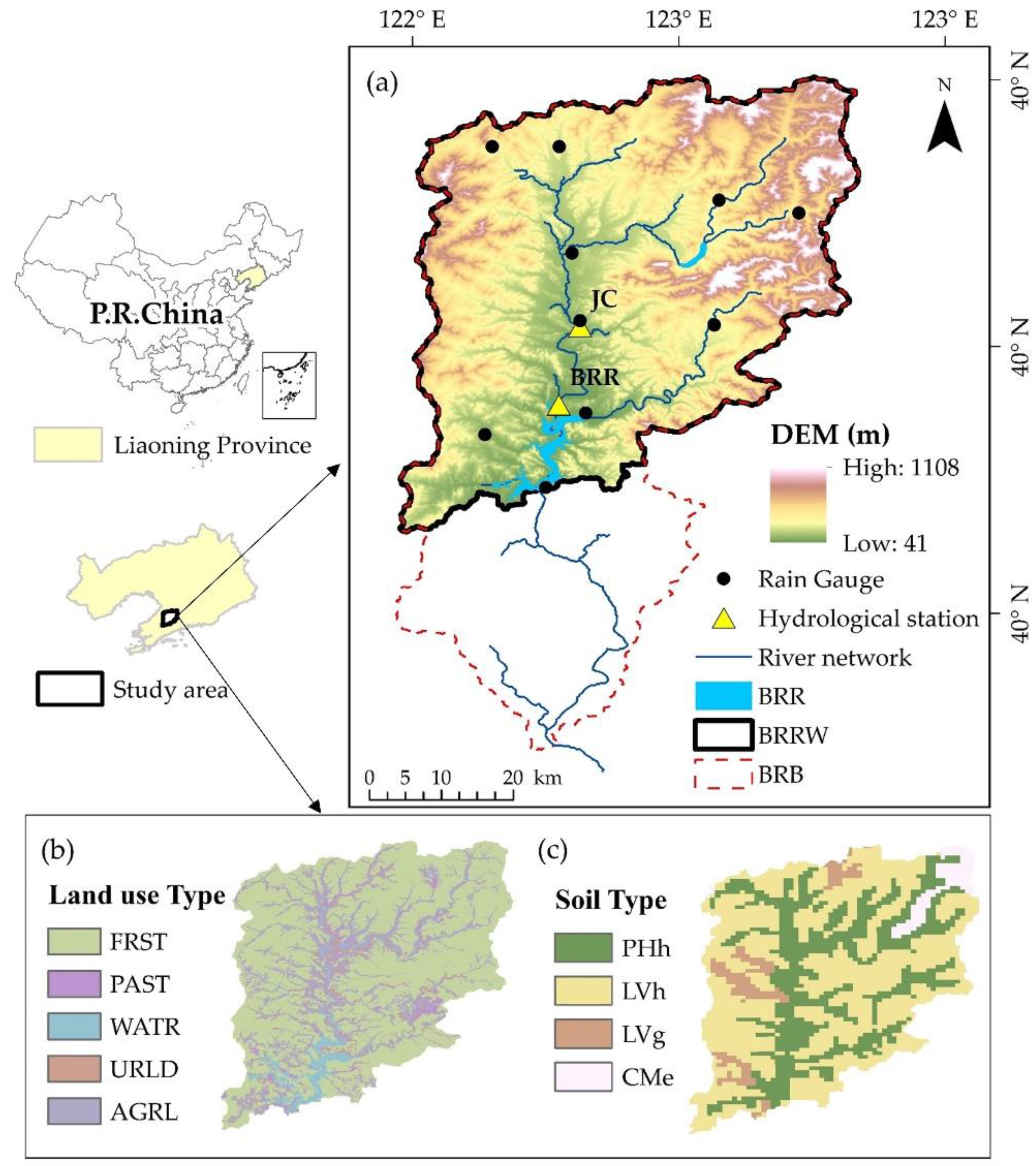
2.1. Study Area

BRRW is located in the upper reach of Biliu River, which is the largest river in Dalian City, Liaoning Province, China (Figure 1a). BRRW is formed by the construction of Biliu River Reservoir (BRR), which is located 66 km downstream from the river head and has a drainage area of 2085 km2, accounting for approximately 74% of the entire Biliu River Basin (BRB). The region has a semi-humid temperate monsoon climate featured with four distinct seasons. The mean annual precipitation is about 739 mm, with more than 70% of the precipitation occurring during the flood season from July to September (see Figure 2 for the spatial distribution of mean annual precipitation). The mean annual air temperature is about 10 °C. January has the coldest mean monthly air temperature at around −8 °C, and July is the warmest month with a mean air temperature of 24 °C. Hilly in the northeast and northwest regions and flat in proximity to the reservoir, the surface elevation ranges from 41 m to 1108 m. Forest (FRST) and agricultural land (AGRL) are the two major land use types covering 72% and 19% of the BRRW, respectively; while pasture (PAST), surface water (WATR) and residential (URLD) occupy the remaining 9% of the total area (Figure 1b). The soils are dominated by Haplic Luvisols (LVh, 60%) and Haplic Phaozems (PHh, 31%) (Figure 1c).
BRR is part of the East-to-West Water Transfer Project of Liaoning Province, which is a vitally important and backbone water conservancy project to the provincial social-economic development. The reservoir has a total storage capacity of 9.3 × 10⁸ m3, and a designed annual water-supply of 4.4 × 10⁸ m3 that serves more than 80% of the domestic and industrial water uses for Dalian city. In addition to water supply, the reservoir has multiple tasks for flood control, power generation, and agricultural irrigation. Therefore, a comprehensive knowledge of the rainfall-runoff hydrological process in BRRW through model simulation and prediction is the guarantee for drinking water-supply and irrigation for millions of people.

2.2. Precipitation Datasets

2.2.1. Gauge Precipitation Data

Observed precipitation is the base to evaluate the performance of satellite precipitation products. Figure 2 shows the locations of eight rain gauges, and their control areas (varying from 166 to 371 km2) following the Thiessen polygon method. Daily precipitation at these gauges from 1 January 2000 to 31 December 2015 are obtained from the Hydrology Bureau of Liaoning Province; data are collected from 0:00 UTC (Coordinated Universal Time) to 24:00 UTC of the current day. The spatial distribution of mean annual precipitation (from 2000 to 2015) of the gauge records, interpolated by the Inverse Distance Weight method, is displayed in Figure 2.

2.2.2. Satellite Precipitation Products

3B42V7 is the latest post real-time data of the TRMM Multi-Satellite Precipitation Analysis (TMPA) product, which is superior to all previous versions [30]. The 3B42V7 dataset is available since January 1998 and covers the global latitude belt from 50° S to 50° N with a spatial resolution of 0.25° × 0.25° and a temporal resolution of 3-h [31]. In this study, the daily precipitation data from 2000 to 2015 are evaluated, which can be downloaded freely from the Goddard Earth Sciences Data and Information Services Center (https://mirador.gsfc.nasa.gov). The daily 3B42V7 data cover an accordant time span from 0:00 UTC to 24:00 UTC with the gauge observation, which are further aggregated into the monthly mean values.
PCDR is maintained by the University of California and National Oceanic and Atmospheric Administration (NOAA) [32]. It is a multi-satellite precipitation product generated by the PERSIANN algorithm using Gridsat-B1 IR satellite data [33]. The product is available since 1983, covering a wider latitude belt from 60°S to 60°N and a same spatial resolution (0.25° × 0.25°) compared with 3B42V7 product. In this study, the daily PCDR data from 2000 to 2015 are obtained from the Center for Hydrometeorology and Remote Sensing (http://chrsdata.eng.uci.edu/).
Though both 3B42V7 and PCDR products are bias-corrected on a monthly basis using the Global Precipitation Climatology Centre (GPCC) dataset [7], none of the eight rain gauges in the study area are included in the GPCC gridded gauge-analysis product. It is therefore essential to examine the accuracy of the two satellite products based on the ground observations, which will be a valuable reference for such semi-humid areas where the satellite precipitation products have been less evaluated.

2.3. Accuracy Assessment of Satellite Precipitation Products

To understand the spatiotemporal variability of 3B42V7 and PCDR against gauge precipitation data, the evaluation at different spatial (i.e., grid scale and watershed scale), and temporal scales (i.e., daily and monthly) are conducted from 2000 to 2015. At the grid scale, the gauge observations are compared with the satellite data of grid where the gauges are located; that are grids No.4, 5, 7, and 8 in Figure 2. Arithmetic average is calculated for gauge data when there is more than one gauge in one satellite grid (e.g., average of five gauges in grid No.5 is compared with the satellite data). As for the watershed-scale comparison, the gauge-based areal precipitation is computed by Thiessen polygons, and the satellite areal precipitation is derived by averaging the satellite data that have more than 50% of its grid inside the watershed (i.e., grids No.4, 5, 7, and 8) [15].
Four basic statistical indices are computed to evaluate the accuracy of satellite-derived precipitation data versus gauge observation. Correction coefficient (CC) is utilized to assess the linear correlation between satellite- and gauge-based precipitation. Root-mean-square error (RMSE) and mean absolute error (MAE) are both used to measure the average error magnitude, whereas the former gives greater weight to large errors. The relative bias (BIAS) represents the systematic bias of satellite precipitation. The above indices are expressed as follows:
CC   = ( P obs , i   P obs ¯ ) ( P sat , i   P sat ¯ ) ( P obs , i   P obs ¯ ) 2 ( P sat , i   P sat ¯ ) 2
RMSE   = 1 n ( P obs , i P sat , i ) 2
MAE   =   1 n | P obs , i P sat , i |  
BIAS   =   ( P sat , i P obs , i ) P obs , i × 100 %
where P obs is the observed precipitation from rain gauge, P sat is the estimated precipitation of 3B42V7 and PCDR products, P obs ¯ and P sat ¯ are the mean values of observed and estimated precipitation, respectively, and n is the number of samples.
To assess the ability of satellite products in detecting precipitation events, three categorical statistical indices, including probability of detection (POD), false alarm ratio (FAR), and critical success index (CSI) are used [34]. A threshold of 1 mm/day is used to differentiate the precipitation and non-precipitation events according to Feidas et al. [35]. The perfect values of POD, FAR, and CSI are 1, 0, and 1, respectively. The formulas are as follows:
POD   = H H + M
FAR   = F H + F
CSI   = H H + M + F
where H is the number of hits (observed rain that was correctly detected), M is the number of misses (observed rain that was not detected), and F is the number of false alarms (rain detected but not observed).

2.4. SWAT Model Application

The SWAT is a time-continuous, semi-distributed, and physically based hydrological model, designed to simulate water, sediment, nutrient, and pesticide transports at a catchment scale on daily, monthly, or yearly time step [36,37,38]. The model divides a watershed into sub-basins connected by the stream network, and further into hydrological response units (HRUs), which is the minimum element to calculate the hydrological processes. The model has been successfully applied in many regions in Northeast China [39,40]. More information about the model can be found in SWAT theoretical documentation [41] and in the literatures [36,42,43].
A variety of data were collected to perform SWAT simulation, including topography, land use, soil types, and meteorological and hydrological conditions. The digital elevation model (DEM) with 90 m resolution was downloaded from National Aeronautics and Space Administration Shuttle Radar Topographic Mission (http://srtm.csi.cgiar.org/). The land cover and soil types with 1 km resolution were obtained from the Data Center for Resources and Environmental Sciences, Chinese Academy of Sciences (http://www.resdc.cn). Daily records of maximum and minimum air temperature, relative humidity, and wind speed were obtained from China Meteorological Administration (http://data.cma.cn). Since there are no meteorological stations inside the study region, the adjacent stations of Xiongyue (122.2°E, 40.18°N), Wafangdian (122.0°E, 39.63°N) and Zhuanghe (123.0°E, 39.7°N) were used, which are approximately 18 km, 31 km, and 33 km away from BRRW, respectively. Daily streamflow at Jianchang (JC) hydrological station during 2000–2015 and the reservoir inflow at BRR station (Figure 1a) during 1986–2015 were obtained from the Biliu River Reservoir Administration; data were further aggregated into monthly averages to evaluate the hydrological model performance.
The BRRB is delineated into 33 sub-basins and further 212 HRUs. Grid centers of satellite products are assumed as virtual meteorological stations to drive the model. The entire simulation is divided into a warm-up period (2000–2001), a calibration period (2002–2009), and a validation period (2010–2015). The SUFI-2 (Sequential Uncertainty Fitting, ver.2) algorithm built in the SWAT-CUP software is employed for sensitivity analysis and auto-calibration [44]. Through sensitive analysis, 13 parameters are selected for model calibration. Three goodness-of-fit measures, namely coefficient of determination (R2), Nash-Sutcliffe Coefficient of Efficiency (NSE) [45], and relative bias radio (Bias) were adopted to evaluate the performance of streamflow simulation, which are expressed as follows:
R 2 = ( ( Q o , i   Q o ¯ ) ( Q m , i   Q m ¯ ) ) 2 ( Q o , i   Q o ¯ ) 2 ( Q m , i   Q m ¯ ) 2
NSE   = 1 ( Q o , i Q m , i ) 2 ( Q o , i Q m ¯ ) 2
Bias =   ( Q m , i Q o , i ) Q o , i × 100 %
where Q o , i and Q m , i represent the observed and simulated streamflow in the ith time period, respectively; Q o ¯ and Q m ¯ represent the average of observed and simulated streamflow, respectively.
To evaluate the application potential of satellite precipitation estimates in hydrological simulation, each of the three precipitation datasets (i.e., ground gauge, 3B42V7, and PCDR) is used independently to drive the model and to obtain their own optimal parameter values. This would be helpful in understanding the accuracy and reliability of the specified satellite data in producing hydrological variables in case it is the sole source of precipitation in the study region. The simulated streamflow and water budget components (i.e., surface runoff, subsurface runoff, groundwater flow, and evapotranspiration) based on different precipitation datasets are analyzed and discussed in Section 3.2 and Section 3.3.

3. Results and Discussion

3.1. Evaluation of Satellite Precipitation Products

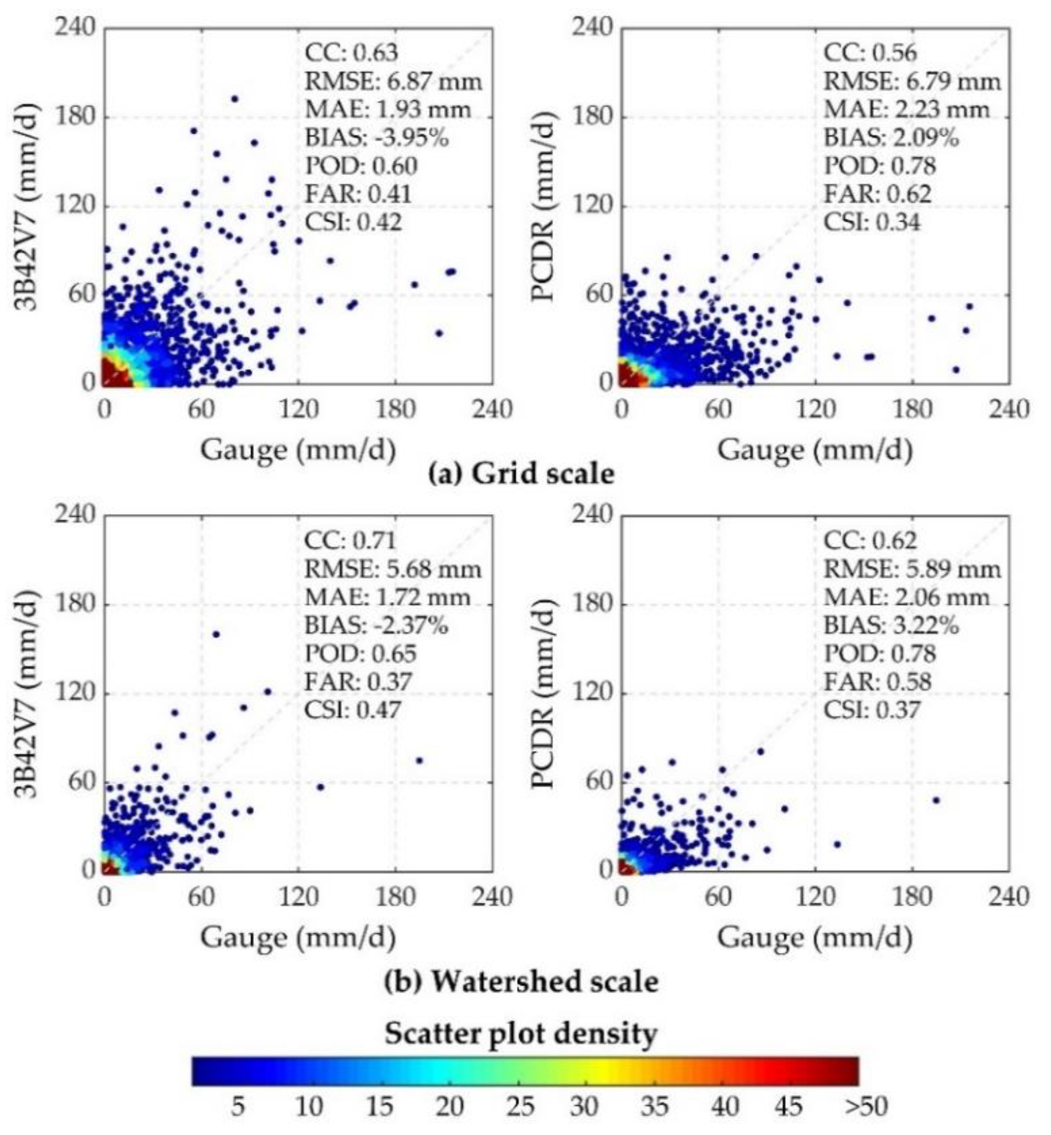
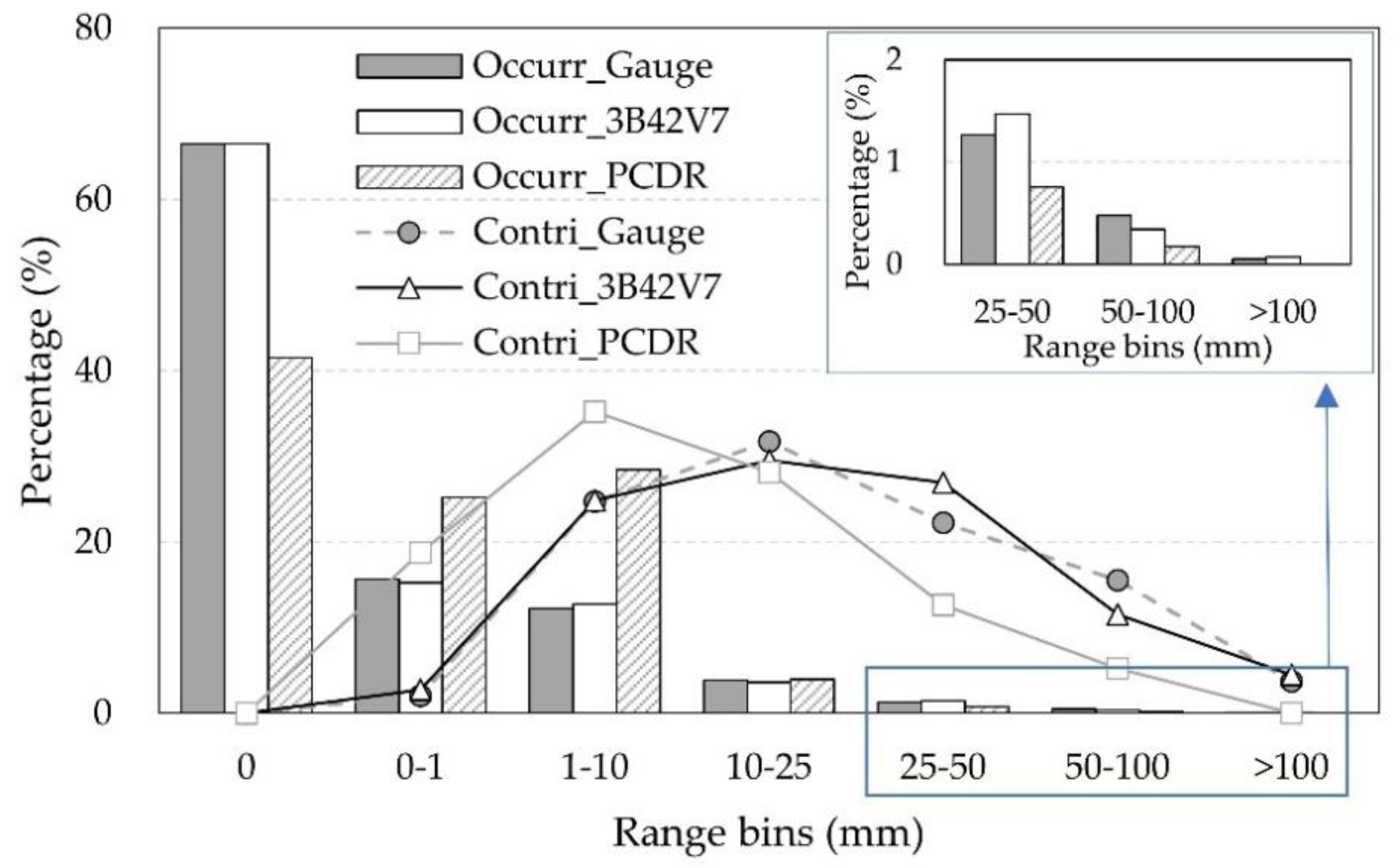
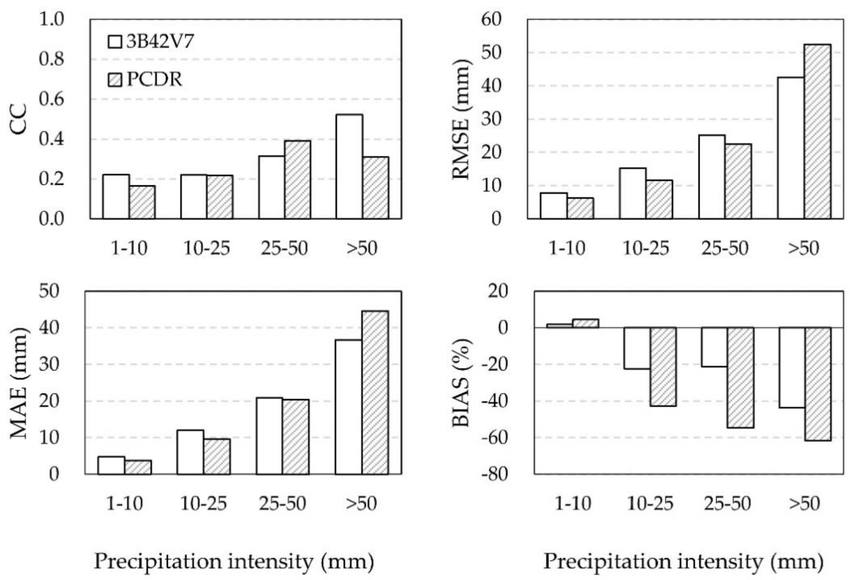
3.1.1. Daily Precipitation

Figure 3 shows the scatter plots of daily data from two satellite products (3B42V7 and PCDR), versus rain gauges at the grid and watershed scales, as well as the corresponding statistical indices. During the evaluation period from 2000 to 2015, there are, in total, 23,376 points for grid-based comparison and 5844 pairs for watershed-based comparison.
At the grid scale, the 3B42V7 and PCDR both had a small BIAS at −3.95% and 2.09%, respectively, indicating an underestimation of 3B42V7 and an overestimation of PCDR overall. 3B42V7 had a larger CC (0.63), and a smaller MAE (1.93 mm) than PCDR (CC: 0.56, MAE: 2.2 3mm); whereas PCDR reported a smaller RMSE (6.79 mm) and a smaller BIAS of 2.09% than 3B42V7 (RMSE: 6.87 mm, BIAS −3.95%). It should be noted that compared to MAE, RMSE retains the difference in magnitude as it can avoid the fact that positive and negative differences cancel each other out, reflecting the randomness of the errors [4,46].
Regarding the contingency of satellite precipitation estimates, 3B42V7 and PCDR both displayed moderate ability in detecting the gauge precipitation events with POD at 0.60 and 0.78, respectively. Although PCDR outperformed 3B42V7 in POD, the higher FAR obviously decreased its overall skill, which showed that 62% of the detected events were false. This further resulted in a lower CSI of PCDR (CSI: 0.34) compared to 3B42V7 (CSI:0.42).
The fitness between satellite data and gauge data differed among grid. As shown in Table 1, grid No.5 generally has a better agreement between the satellite-based and gauge-based data, as indicated by the higher CC and CSI, and smaller RMSE, MAE, and FAR. This is probably attributed to the five gauge stations scattered over the grid that can better represent the areal precipitation within this grid. As reminded by previous studies [14,47], the gauge observations that are usually used as reference datasets may be subject to uncertainties due to errors in recording and deficits of regionalization, and the rain gauges density may affect the evaluation results.
At the watershed scale, both 3B42V7 and PCDR showed a better agreement compared with the grid scale, because all statistical indices are closer to their corresponding perfect values, except for the BIAS of PCDR. In general, 3B42V7 outperformed PCDR at both spatial scales, as indicated by the higher CC and CSI, and smaller RMSE (for watershed scale only), MAE, BIAS, and FAR of 3B42V7 dataset.
Additionally, it is generally recognized that the distribution pattern of precipitation with different intensities is an important feature and has significant effects on streamflow modeling and flood forecasting [48,49]. Therefore, the occurrence frequency of daily precipitation and the corresponding contribution to the total precipitation are evaluated for different intensities at the watershed scale (Figure 4).
It can be seen that the “non-rainy” days (0 mm) was the class that most frequently occurred, with an occurrence rate of 66.5% for gauge observation and 3B42V7, and 41.5% for PCDR. The second largest class was “0–1 mm” for the gauge and 3B42V7 data, occurring in 15.6% and 15.2% of the total number of days, respectively, followed by the class of “1–10 mm”, occurring in 12.3% and 12.8%, respectively. In general, the 3B42V7 under “non-rainy” and “light rain” classes had a similar occurrence rate compared to the gauge data. This is different with some previous studies, stating that TMPA product is less effective in correctly specifying the moderate and light rain rates [2,15].
However, for PCDR, more “0–1 mm” (occurrence rate: 25.2%)” and “1–10 mm” (occurrence rate: 28.5%) days were recorded compared to gauge observation. The discrepancies were also evident in the contribution pattern, where PCDR had an overestimation in light rainfall class (0–1 mm and 1–10 mm) and an underestimation in high rainfall classes (>25 mm). Similar findings on the performance of PCDR were reported in Northeastern China [50], the contiguous United States [33], and Italy [51]. Besides, no events above 100 mm were recorded in PCDR, while both the gauge and 3B42V7 data had two events larger than 100 mm, reflecting an inadequate ability of PCDR in detecting extreme precipitation events. The 3B42V7, however, showed a similar contribution pattern against the gauge data for all classes, with an acceptable discrepancy within ±5%, indicating that the 3B42V7 data is more adequate in characterizing the rainfall structure of the gauge observation.
Further, the performance of daily precipitation of 3B42V7 and PCDR products under different rainfall intensities was assessed at the watershed scale (Figure 5). Four indices, i.e., CC, RMSE, MAE, and BIAS, were applied for comparison. CC increased from 0.20 to 0.42 (on average of the two products) as the rainfall intensity increased; whereas RMSE, MAE, and BIAS indicated a falling performance of both satellite-based products as the rainfall intensity increased. The performances of two satellite products differed in terms of rainfall intensities. 3B42V7 showed better agreement in torrential rains (>50 mm), whereas PCDR preceded in heavy rainfall events (25–50 mm) except for the BIAS index. As for light (1–10 mm) and moderate (10–25 mm) events, performances of the two products were comparable as indicated by the larger CC and smaller bias for 3B42V7, and the smaller RMSE and MAE for PCDR.

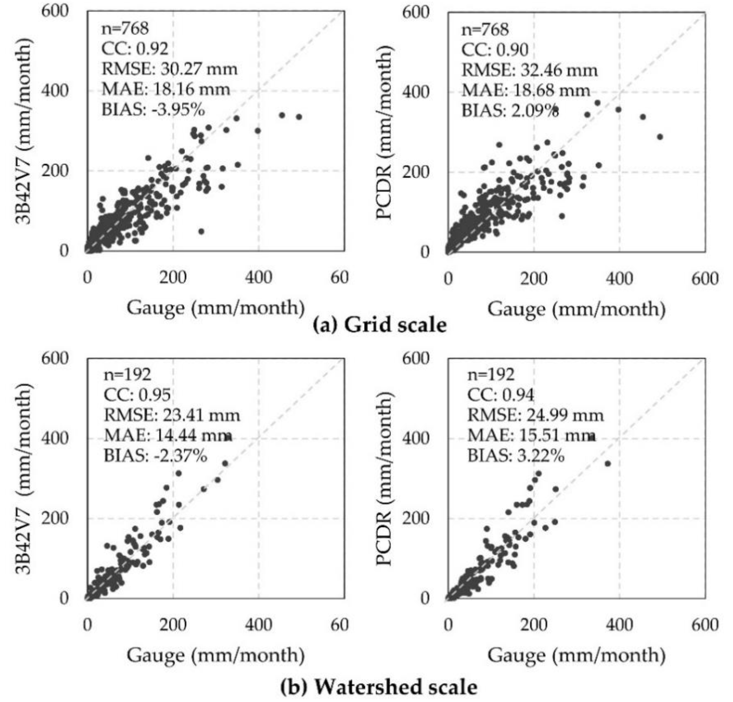
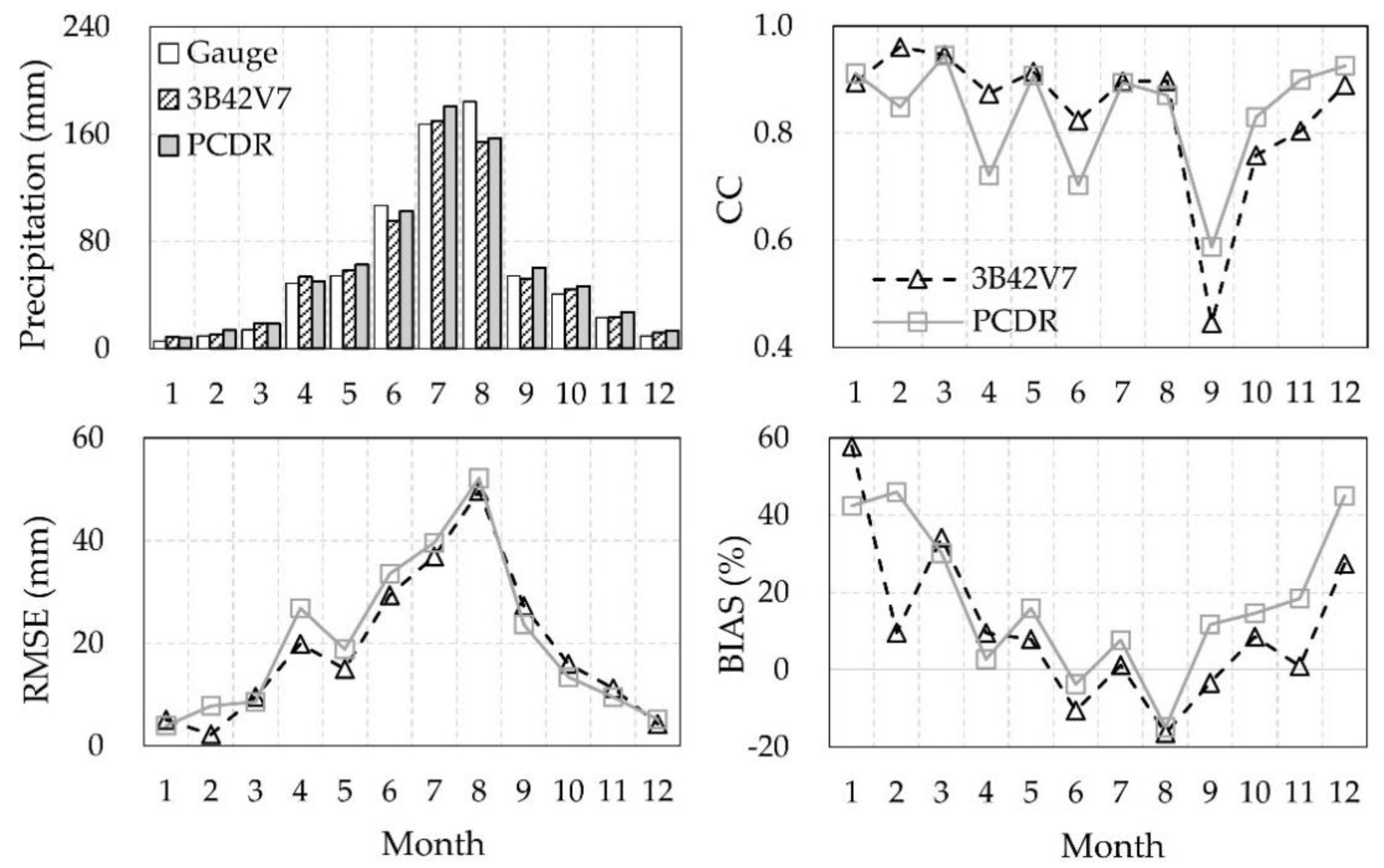
3.1.2. Monthly Precipitation

Figure 6 shows the comparison results of monthly satellite precipitation and gauge data. The assessment on the capability in detecting precipitation events is not able to perform at the monthly scale, because all months of the three datasets have precipitations larger than 1 mm. The correlation relationship is greatly improved at the monthly scale. The CC values were larger than 0.90 for both products at the grid and watershed scales.
Due to the intra-annual variabilities of precipitation, the performance of satellite products for each month is further evaluated. Figure 7 shows the statistical indices of CC, RMSE, and BIAS for each month. Overall, both 3B42V7 and PCDR can capture the monthly precipitation pattern of the gauge observation. The linear relationships were satisfactory with the CC above 0.80 for 3B42V7 and above 0.70 for PCDR during all months except for September. RMSE increased as the monthly precipitation increased, with the maximum RMSE occurred in August for both satellite products. The variations in BIAS showed clearly the underestimation during the high-precipitation period from June to September (for PCDR only in June and August), while overestimation during other months. It is worthy to recognize that the systematic errors were relatively small in the wet season (i.e., from June to September) with the absolute values of BIAS lower than 20%, while large in the dry season (i.e., from December to next March) with a BIAS up to 60%. In general, 3B42V7 produced a smaller absolute value of BIAS throughout the year (10.6% for 3B42V7 and 18.1% for PCDR on average), and was slightly superior in CC and RMSE from January to August; while PCDR outperformed 3B42V7 from September to December as indicated by its larger CC and smaller RMSE.

3.2. Evaluation of Streamflow Simulation

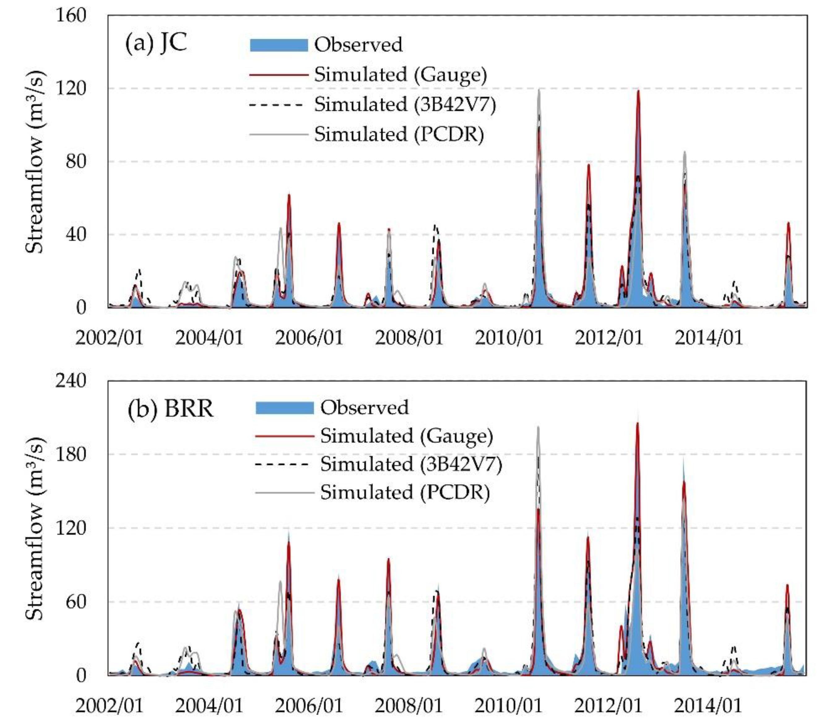
3.2.1. Streamflow Simulation

Table 2 shows the calibrated values of 13 parameters, and all values lie within their proper ranges. Figure 8 shows the observed and simulated monthly streamflow at JC and BRR stations (Figure 1a); the corresponding statistical indices are summarized in Table 3.
The simulated streamflow driven by gauge data exhibited a closer agreement with the observed data than model simulations using 3B42V7 and PCDR data. The NSE and R2 were particularly high for the gauge-based simulation; the NSE ranged from 0.92 to 0.96, and R2 ranged from 0.93 to 0.97. The good fitness demonstrates that the model is capable of capturing the key features of the observed hydrograph at monthly scale when forced by gauge precipitation. Therefore, the model is considered robust and provides a sound basis for further testing the precision and applicability of satellite products.
The model performances driven by two satellite products were lower than the gauge-based simulation. At BRR station, 3B42V7-based model led to a slightly better model efficiency and a lower systematic error than PCDR, as indicated by a larger NSE of 0.76 (PCDR: 0.65), a larger R2 of 0.77 (PCDR: 0.67), and a smaller Bias of 18.3% (PCDR: 22.9%) on average during calibration and validation periods. Similarly, 3B42V7 outperformed PCDR in producing the streamflow at JC station, with the NSE of 0.68 and 0.56, R2 of 0.70 and 0.59, and Bias of 9.8% and 17.4% for 3B42V7 and PCDR, respectively. Overall, consistent with the quality evaluation of the two satellite products, 3B42V7 exhibited a better performance than PCDR in depicting streamflow hydrographs.

3.2.2. Performance under Different Flow Levels and Hydrological Years

In addition to the overall hydrographs, the ability of capturing the flow peaks and low flow conditions are of particular importance for flood control and drought prevention. To investigate the model performance at different flow levels, the monthly observed streamflow exceeding its 90% quantile is defined as high flow and that less than its 50% quantile is defined as low flow; the streamflow between these two is defined as moderate flow. On this basis, the entire study period is divided into 16 months of high flow, 84 months of moderate flow, and 68 months of low flow. The statistical indices of streamflow simulation under different flow conditions are summarized in Table 4.
Under the high flow condition, the gauge-based model generated a perfect simulation result with R2 of 0.92 and 0.85 at JC and BRR, respectively. The calculated Bias was also small within a range of ±10%. However, both 3B42V7- and PCDR-based models yielded an underestimation of streamflow, as indicated by the negative Bias ranging from −13.8% to −28.4%. Model performance using 3B42V7 data was better than that using PCDR, with a larger R2 of 0.63 and 0.54 at JC and BRR, respectively, and a smaller Bias of −13.8% and −21.7% at JC and BRR, respectively. The better performance of 3B42V7-based model during high flow condition is probably due to the better representation of 3B42V7 in capturing torrential rains (Figure 4 and Figure 5).
As regards to the moderate flow, the gauge-based model generated a satisfactory R2 of 0.69 and 0.74 at JC and BRR, respectively, but a larger Bias of −30% at BRR. The model performances utilizing 3B42V7 and PCDR data were relatively lower. The R2 ranged from 0.16 to 0.27, and the Bias was larger than 40% at JC whereas lower within −10% at BRR. Therefore, the gauge observations are more accurate in depicting runoff process under moderate flow conditions; whereas, the satellite products match well in the amount of streamflow (at BRR only). Unfortunately, at the low flow level, model simulations driven by the three precipitation datasets all produced unsatisfactory results, with R2 ranging from 0.01 to 0.29, and absolute values of Bias larger than 35% (except for gauge-based simulation at JC). As demonstrated in previous studies, the poor performance under relatively low flow levels may be attributable to the uncertainties of other input data (such as soil type) and parameters, as well as the limitation of SWAT internal algorithms under low-flow conditions [52,53]. Therefore, reliable precipitation data, along with improved model algorithms, are both essential to enable a more accurate and realistic streamflow simulation [54].
The performances of satellite precipitation datasets in generating streamflow are also evaluated at different hydrological years. Prior to evaluation, the historical sequence of streamflow at BRR station during 1986 to 2015 is used to plot the annual runoff frequency curve. Then the annual runoff frequency (F) of 37.5% and 62.5% are adopted as the classification standard [55,56], and the 16-year simulation period is divided into wet years (F ≤ 37.5%, including years of 2005, and 2010 to 2013), normal years (37.5% < F ≤ 62.5%, including years of 2004, 2006, 2007, 2008, and 2015) and dry years (F > 62.5%, including years of 2002, 2003, 2009, and 2014).
Table 5 lists the evaluation indices of streamflow simulation during the wet, normal and dry years. The gauge-based model gained preferable results than 3B42V7-and PCDR- based models for all indices, with R2 above 0.9 for the wet and normal years, and above 0.5 for the dry years. Generally, simulation results got worse as the frequency increased, as indicated by the decreased R2 and increased absolute values of Bias. The performances of 3B42V7-and PCDR- based models were satisfactory during the wet and normal years, with R2 ranging from 0.54 to 0.83; however, they yielded remarkable underestimation at BRR, with Bias ranging from −17.1% to −32.8%. Generally, 3B42V7 produced a relatively better performance than PCDR in wet years with larger R2 and smaller Bias, while the performance of these two products were comparable in the normal years. In the dry years, both 3B42V7- and PCDR-based simulations showed poorer correlations with the observed streamflow.

3.3. Evaluation of Hydrologic Process Simulation

3.3.1. Water Balance

In addition to streamflow predictions, the ability in producing hydrological variables is another important indicator for assessing the satellite precipitation data [3]. Water balance analysis was carried out to compare the major components of hydrological cycle from monthly simulations driven by the three precipitation datasets. The SWAT model partitions precipitation into evaporation, transpiration, ground discharge (including base flow), and runoff (including surface runoff, base flow, and subsurface flow) [38]. Numerical comparisons of the averaged water balance components from 2002 to 2015 are shown in Table 6.
In the case of gauge-based simulation, 73.5% of precipitation was exhausted through evaporation and transpiration, and a very similar rate of 73.6% was produced by 3B42V7; whereas the corresponding rate in PCDR was slightly overestimated (75%). As a key component determining the amount of base flow, the groundwater recharge accounted for 13.9%, 10.5%, and 19% of precipitation in the gauge-, 3B42V7- and PCDR-driven simulations, respectively. As for the total runoff, the 3B42V7-based model generated a similar total runoff to the gauge-based model, 198.7 mm and 186.2 mm, respectively. Less total runoff was produced in the PCDR case (155.8 mm), although the precipitation estimate of PCDR was larger than that of gauge observation and 3B42V7 estimate, probably due to the overestimated exhaust through evaporation, transpiration and groundwater recharge. The differences in runoff components were notable between PCDR- and gauge-based models, especially for the surface runoff, (i.e., 86.1 mm for gauge and 18.1 mm for PCDR), and the base flow volume (i.e., 79.9 mm for gauge and 110.0 mm for PCDR).

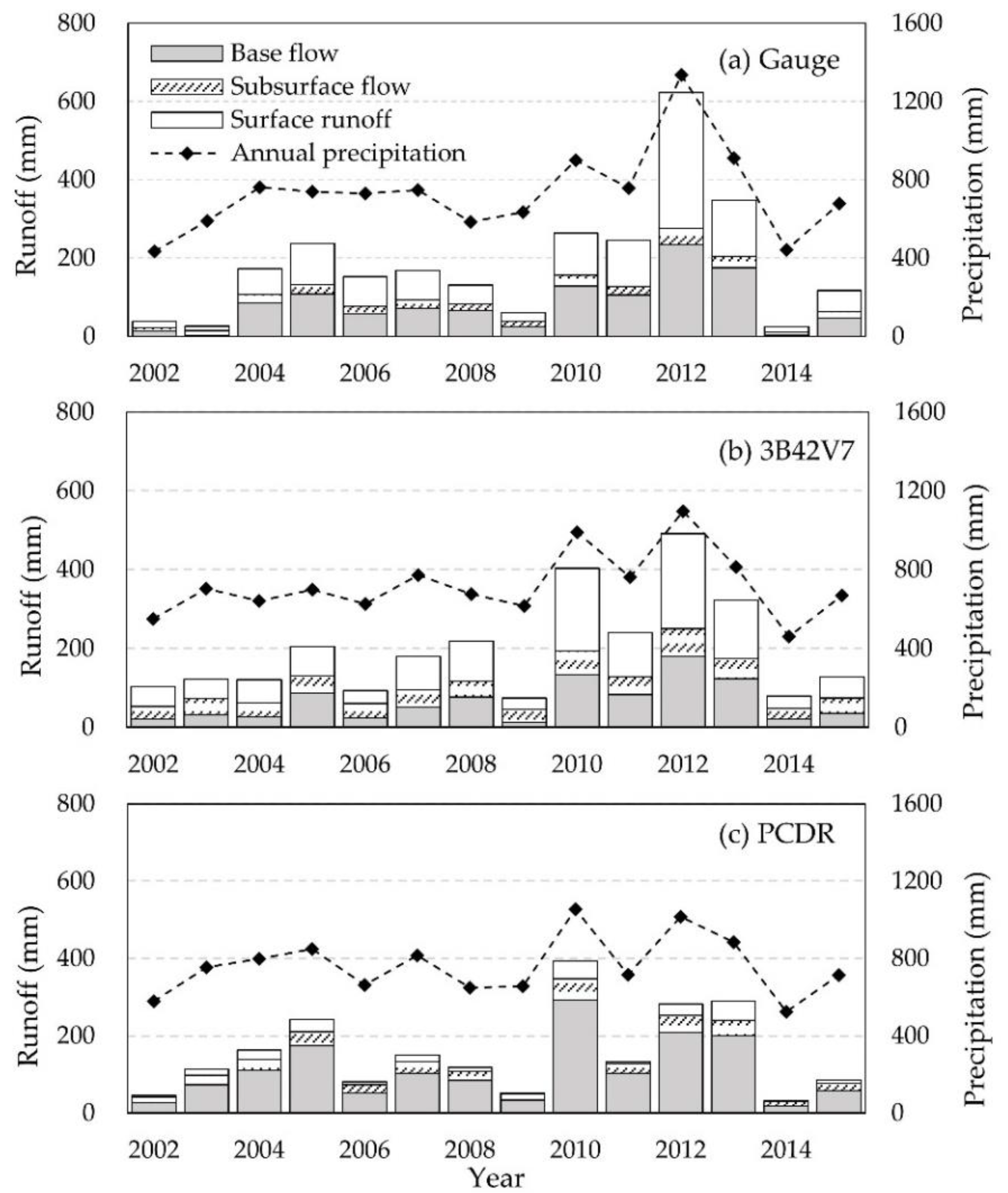
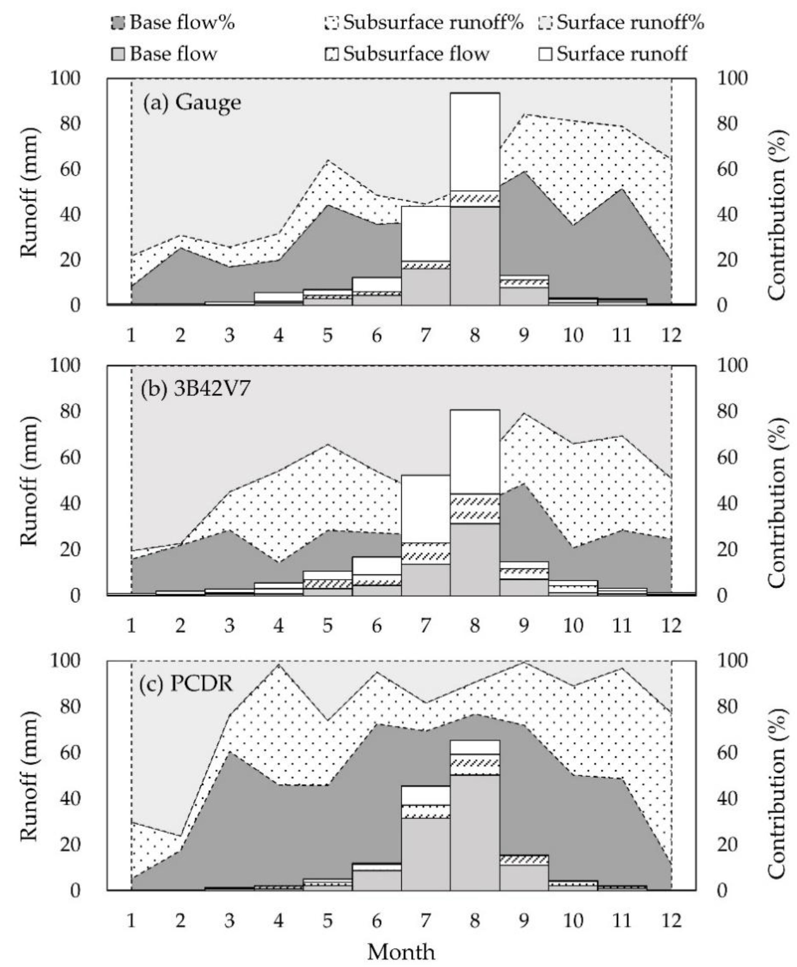
3.3.2. Annual and Monthly Runoff Distributions

The runoff distributions (i.e., monthly and annually) and components (i.e., surface flow, subsurface flow, and base flow) are of great concerns in evaluating the water resources from different sources. Figure 9 displays the annual total runoff partitioning into surface runoff, base flow and subsurface flow from 2002 to 2015. Generally, two satellite datasets captured well the overall trends of annual precipitation and total runoff. Both gauge- and 3B42V7-based results indicated that surface runoff was the dominant contributor to total runoff, followed by base flow, while PCDR led to an overestimation in base flow simulation and an underestimation in surface runoff simulation.
Figure 10 further displays the compositions of monthly runoff driven by gauge, 3B42V7 and PCDR data. The monthly variations of total runoff were consistent among the three simulations, with more than two thirds of total runoff occurring in July and August. In general, 3B42V7 generated a similar contribution pattern with the gauge-based simulation; that is, surface runoff was the dominate component from January to August, and subsurface flow and base flow became the major contributors during September to December. Unfortunately, PCDR was not able to produce the intra-annual runoff compositions, which tended to overestimate the base flow most of the time from March to November and underestimate the role of surface flow.

4. Conclusions

This study assessed the accuracy of two satellite precipitation products, i.e., 3B42V7 and PCDR, and their utilities in driving hydrological simulation over a semi-humid region in the Biliu River Reservoir Watershed (China).
Results indicated that 3B42V7 generally outperformed PCDR in estimating the gauge precipitation. Performance of both satellite products improved with the time and space aggregations from daily to monthly scale, and from grid to watershed scale. The abilities in detecting precipitation events were comparable between the two satellite datasets. Dividing the precipitation into different intensities, it was found that 3B42V7 was superior in determining the rainfall occurrence under all intensities, whereas PCDR overestimated the light rainfall (1–10 mm) and underestimated the moderate (10–25 mm) and high rainfalls (>25 mm). Evaluation indices for different grids showed a better agreement between the daily satellite estimates and gauge precipitation in a data-rich grid. Therefore, it is worth to thicken the network of precipitation measurements with further precipitation stations, which would increase the amount of data necessary in the validation processes in the future.
The R2, NSE, and Bias were applied to evaluate the monthly hydrological model performance. The 3B42V7-based simulation showed a better agreement between the simulated and observed streamflow compared to model simulation using PCDR. Specifically, the gauge data were well suited for simulating the high and moderate flows, and 3B42V7 data were also applicable in the high flow simulation. However, neither 3B42V7 nor PCDR were capable in modeling the moderate and low flow conditions. Further, water balance analysis indicated that the 3B42V7 data and gauge observations denoted very similar water balance and runoff compositions, while PCDR overestimated the base flow and underestimated the surface flow most of the time. Overall, results in this study suggested the adequacy and applicability of 3B42V7 in describing hydrological features in the study area, which is vital in water resources planning and management in case there is less gauge-based observation.
To date, there are more than 30 global precipitation datasets available that can serve as alternative precipitation data sources including gauge-based, reanalysis, and satellite data [57]. Although many of them are proven to have great potential in the real hydrological applications, there is still much room to improve the accuracy of satellite products for various hydrologic purposes, such as flood forecasting, drought prevention, and water supply. Therefore, further studies need to carry out the in-depth work of satellite precipitation correction and validation over different parts of the world, in order for decision-makers to find alternative precipitation sources for water resources planning and management.

Author Contributions

All authors contributed extensively to the work presented in this paper. L.Z. performed the experiment and prepared the manuscript draft. Z.X. helped to design the framework of this study and revise the manuscript. H.Z. provided valuable suggestions. All authors have read and agreed to the published version of the manuscript.

Funding

This research was funded by the National Key Research and Development Program, grant number 2017YFC0406001; and the National Natural Science Foundation of China, grant numbers 51809031, 51925902.

Acknowledgments

The authors acknowledge the Hydrology Bureau of Liaoning Province, the Biliu River Reservoir Administration, and the TMPA and PERSIANN-CDR products developer for providing the data in this study. We also thank the reviewers for their constructive suggestions.

Conflicts of Interest

The authors declare no conflict of interest.

References

  1. Masih, I.; Maskey, S.; Uhlenbrook, S.; Smakhtin, V. Assessing the impact of areal precipitation input on streamflow simulations using the SWAT model. J. Am. Water Resour. Assoc. 2011, 47, 179–195. [Google Scholar]
  2. Michaelides, S.; Levizzani, V.; Anagnostou, E.; Bauer, P.; Kasparis, T.; Lane, J.E. Precipitation: Measurement, remote sensing, climatology and modeling. Atmos. Res. 2009, 94, 512–533. [Google Scholar]
  3. Xu, H.; Xu, C.; Chen, H.; Zhang, Z.; Li, L. Assessing the influence of rain gauge density and distribution on hydrological model performance in a humid region of China. J. Hydrol. 2013, 505, 1–12. [Google Scholar]
  4. Deng, P.; Zhang, M.; Bing, J.; Jia, J.; Zhang, D. Evaluation of the GSMaP_Gauge products using rain gauge observations and SWAT model in the Upper Hanjiang River Basin. Atmos. Res. 2019, 219, 153–165. [Google Scholar]
  5. Yu, Z.; Wu, J.; Chen, X. An approach to revising the climate forecast system reanalysis rainfall data in a sparsely-gauged mountain basin. Atmos. Res. 2019, 220, 194–205. [Google Scholar]
  6. Mei, Y.; Nikolopoulos, E.I.; Anagnostou, E.N.; Borga, M. Evaluating Satellite Precipitation Error Propagation in Runoff Simulations of Mountainous Basins. J. Hydrometeorol. 2016, 17, 1407–1423. [Google Scholar]
  7. Yuan, F.; Zhang, L.; Win, K.; Ren, L.; Zhao, C.; Zhu, Y.; Jiang, S.; Liu, Y. Assessment of GPM and TRMM Multi-Satellite Precipitation Products in Streamflow Simulations in a Data-Sparse Mountainous Watershed in Myanmar. Remote Sens. 2017, 9, 302. [Google Scholar]
  8. Tan, J.; Petersen, W.A.; Tokay, A. A Novel Approach to Identify Sources of Errors in IMERG for GPM Ground Validation. J. Hydrometeorol. 2016, 17, 2477–2491. [Google Scholar]
  9. Bitew, M.M.; Gebremichael, M. Assessment of satellite rainfall products for streamflow simulation in medium watersheds of the Ethiopian highlands. Hydrol. Earth Syst. Sci. 2011, 15, 1147–1155. [Google Scholar]
  10. Li, X.; Zhang, Q.; Xu, C. Suitability of the TRMM satellite rainfalls in driving a distributed hydrological model for water balance computations in Xinjiang catchment, Poyang lake basin. J. Hydrol. 2012, 426–427, 28–38. [Google Scholar]
  11. Zhang, Z.; Tian, J.; Huang, Y.; Chen, X.; Chen, S.; Duan, Z. Hydrologic Evaluation of TRMM and GPM IMERG Satellite-based Precipitation in a Humid Basin of China. Remote Sens. 2019, 11, 431. [Google Scholar] [CrossRef] [Green Version]
  12. Yu, M.; Chen, X.; Li, L.; Bao, A.; De la Paix, M.J. Streamflow simulation by SWAT using different precipitation sources in large arid basins with scarce raingauges. Water Resour. Manag. 2011, 25, 2669. [Google Scholar] [CrossRef]
  13. Himanshu, S.K.; Pandey, A.; Patil, A. Hydrologic Evaluation of the TMPA-3B42V7 Precipitation Data Set over an Agricultural Watershed Using the SWAT Model. J. Hydrol. Eng. 2018, 23, 5018003. [Google Scholar] [CrossRef]
  14. Zhu, Q.; Xuan, W.; Liu, L.; Xu, Y. Evaluation and hydrological application of precipitation estimates derived from PERSIANN-CDR, TRMM 3B42V7, and NCEP-CFSR over humid regions in China. Hydrol. Process. 2016, 30, 3061–3083. [Google Scholar] [CrossRef]
  15. Li, D.; Christakos, G.; Ding, X.; Wu, J. Adequacy of TRMM satellite rainfall data in driving the SWAT modeling of Tiaoxi catchment (Taihu lake basin, China). J. Hydrol. 2018, 556, 1139–1152. [Google Scholar] [CrossRef]
  16. Vu, T.; Li, L.; Jun, K. Evaluation of Multi-Satellite Precipitation Products for Streamflow Simulations: A Case Study for the Han River Basin in the Korean Peninsula, East Asia. Water 2018, 10, 642. [Google Scholar] [CrossRef] [Green Version]
  17. Tan, M.; Samat, N.; Chan, N.; Roy, R. Hydro-Meteorological Assessment of Three GPM Satellite Precipitation Products in the Kelantan River Basin, Malaysia. Remote Sens. 2018, 10, 1011. [Google Scholar] [CrossRef] [Green Version]
  18. Beck, H.E.; Vergopolan, N.; Pan, M.; Levizzani, V.; van Dijk, A.I.J.M.; Weedon, G.P.; Brocca, L.; Pappenberger, F.; Huffman, G.J.; Wood, E.F. Global-scale evaluation of 22 precipitation datasets using gauge observations and hydrological modeling. Hydrol. Earth Syst. Sci. 2017, 21, 6201–6217. [Google Scholar] [CrossRef] [Green Version]
  19. Guo, H.; Chen, S.; Bao, A.; Hu, J.; Gebregiorgis, A.; Xue, X.; Zhang, X. Inter-Comparison of High-Resolution Satellite Precipitation Products over Central Asia. Remote Sens. 2015, 7, 7181–7211. [Google Scholar] [CrossRef] [Green Version]
  20. Muhammad, E.; Muhammad, W.; Ahmad, I.; Muhammad Khan, N.; Chen, S. Satellite precipitation product: Applicability and accuracy evaluation in diverse region. Sci. China Technol. Sci. 2020, 63, 819–828. [Google Scholar] [CrossRef]
  21. Alnahit, A.O.; Mishra, A.K.; Khan, A.A. Evaluation of high-resolution satellite products for streamflow and water quality assessment in a Southeastern US watershed. J. Hydrol. Reg. Stud. 2020, 27, 100660. [Google Scholar] [CrossRef]
  22. Tang, X.; Zhang, J.; Gao, C.; Ruben, G.; Wang, G. Assessing the Uncertainties of Four Precipitation Products for Swat Modeling in Mekong River Basin. Remote Sens. 2019, 11, 304. [Google Scholar] [CrossRef] [Green Version]
  23. Ma, D.; Xu, Y.; Gu, H.; Zhu, Q.; Sun, Z.; Xuan, W. Role of satellite and reanalysis precipitation products in streamflow and sediment modeling over a typical alpine and gorge region in Southwest China. Sci. Total Environ. 2019, 685, 934–950. [Google Scholar] [CrossRef]
  24. Le, M.; Lakshmi, V.; Bolten, J.; Bui, D.D. Adequacy of Satellite-derived Precipitation Estimate for Hydrological Modeling in Vietnam Basins. J. Hydrol. 2020, 586, 124820. [Google Scholar] [CrossRef]
  25. Jiang, S.; Ren, L.; Xu, C.; Yong, B.; Yuan, F.; Liu, Y.; Yang, X.; Zeng, X. Statistical and hydrological evaluation of the latest Integrated Multi-satellitE Retrievals for GPM (IMERG) over a midlatitude humid basin in South China. Atmos. Res. 2018, 214, 418–429. [Google Scholar] [CrossRef]
  26. Zhang, D.; Liu, X.; Bai, P.; Li, X. Suitability of Satellite-Based Precipitation Products for Water Balance Simulations Using Multiple Observations in a Humid Catchment. Remote Sens. 2019, 11, 151. [Google Scholar] [CrossRef] [Green Version]
  27. Zhu, H.; Li, Y.; Huang, Y.; Li, Y.; Hou, C.; Shi, X. Evaluation and hydrological application of satellite-based precipitation datasets in driving hydrological models over the Huifa river basin in Northeast China. Atmos. Res. 2018, 207, 28–41. [Google Scholar] [CrossRef]
  28. Cai, Y.; Jin, C.; Wang, A.; Guan, D.; Wu, J.; Yuan, F.; Xu, L. Comprehensive precipitation evaluation of TRMM 3B42 with dense rain gauge networks in a mid-latitude basin, northeast, China. Theor. Appl. Climatol. 2016, 126, 659–671. [Google Scholar] [CrossRef]
  29. Zhang, Q.; Xu, C.; Yang, T. Variability of water resource in the Yellow River basin of past 50 years, China. Water Resour. Manag. 2009, 23, 1157–1170. [Google Scholar] [CrossRef]
  30. Yong, B.; Chen, B.; Gourley, J.J.; Ren, L.; Hong, Y.; Chen, X.; Wang, W.; Chen, S.; Gong, L. Intercomparison of the Version-6 and Version-7 TMPA precipitation products over high and low latitudes basins with independent gauge networks: Is the newer version better in both real-time and post-real-time analysis for water resources and hydrologic extremes? J. Hydrol. 2014, 508, 77–87. [Google Scholar]
  31. Huffman, G.J.; Bolvin, D.T.; Nelkin, E.J.; Wolff, D.B.; Adler, R.F.; Gu, G.; Hong, Y.; Bowman, K.P.; Stocker, E.F. The TRMM Multisatellite Precipitation Analysis (TMPA): Quasi-Global, Multiyear, Combined-Sensor Precipitation Estimates at Fine Scales. J. Hydrometeorol. 2007, 8, 38–55. [Google Scholar] [CrossRef]
  32. Hsu, K.; Gao, X.; Sorooshian, S.; Gupta, H.V. Precipitation estimation from remotely sensed information using artificial neural networks. J. Appl. Meteorol. 1997, 36, 1176–1190. [Google Scholar] [CrossRef]
  33. Ashouri, H.; Hsu, K.; Sorooshian, S.; Braithwaite, D.K.; Knapp, K.R.; Cecil, L.D.; Nelson, B.R.; Prat, O.P. PERSIANN-CDR: Daily Precipitation Climate Data Record from Multisatellite Observations for Hydrological and Climate Studies. Bull. Am. Meteorol. Soc. 2015, 96, 69–83. [Google Scholar] [CrossRef] [Green Version]
  34. Ebert, E.E.; Janowiak, J.E.; Kidd, C. Comparison of Near-Real-Time Precipitation Estimates from Satellite Observations and Numerical Models. Bull. Am. Meteorol. Soc. 2007, 88, 47–64. [Google Scholar] [CrossRef] [Green Version]
  35. Feidas, H.; Porcu, F.; Puca, S.; Rinollo, A.; Lagouvardos, C.; Kotroni, V. Validation of the H-SAF precipitation products over Greece using rain gauge data. Theor. Appl. Climatol. 2018, 377–398. [Google Scholar] [CrossRef]
  36. Arnold, J.G.; Srinivasan, R.; Ramanarayanan, T.S.; Arnold, J.G.; Bednarz, S.T. Large area dyrologic modeling and assessment, Part 1: Model development. J. Am. Water Resour. Assoc. 1998, 1, 73–89. [Google Scholar]
  37. Morgan, R.P.C. A simple approach to soil loss prediction: A revised Morgan–Morgan–Finney model. Catena 2001, 44, 305–322. [Google Scholar] [CrossRef]
  38. Neitsch, S.L.; Arnold, J.G.; Kiniry, J.R.; Williams, J.R.; King, K.W. Soil and Water Assessment Tool Theoretical Documentation; Version 2005; USDA-ARS Grassland: Temple, TX, USA, 2005; Volume 8. [Google Scholar]
  39. Feng, X.Q.; Zhang, G.X.; Jun Xu, Y. Simulation of hydrological processes in the Zhalong wetland within a river basin, Northeast China. Hydrol. Earth Syst. Sci. 2013, 17, 2797–2807. [Google Scholar]
  40. Zhang, A.; Zhang, C.; Fu, G.; Wang, B.; Bao, Z.; Zheng, H. Assessments of impacts of climate change and human activities on runoff with SWAT for the Huifa River Basin, Northeast China. Water Resour. Manag. 2012, 26, 2199–2217. [Google Scholar]
  41. Arnold, J.G.; Moriasi, D.N.; Gassman, P.W.; Abbaspour, K.C.; White, M.J.; Srinivasan, R.; Santhi, C.; Harmel, R.D.; Van Griensven, A.; Van Liew, M.W. SWAT: Model use, calibration, and validation. Trans. ASABE 2012, 55, 1491–1508. [Google Scholar]
  42. Green, C.; van Griensven, A. Autocalibration in hydrologic modeling: Using SWAT2005 in small-scale watersheds. Environ. Model. Softw. 2008, 23, 422–434. [Google Scholar] [CrossRef]
  43. Abbaspour, K.C.; Rouholahnejad, E.; Vaghefi, S.; Srinivasan, R.; Yang, H.; Kløve, B. A continental-scale hydrology and water quality model for Europe: Calibration and uncertainty of a high-resolution large-scale SWAT model. J. Hydrol. 2015, 524, 733–752. [Google Scholar] [CrossRef] [Green Version]
  44. Abbaspour, K.C.; Yang, J.; Maximov, I.; Siber, R.; Bogner, K.; Mieleitner, J.; Zobrist, J.; Srinivasan, R. Modelling hydrology and water quality in the pre-alpine/alpine Thur watershed using SWAT. J. Hydrol. 2007, 333, 413–430. [Google Scholar] [CrossRef]
  45. Nash, J.E.; Sutcliffe, J.V. River flow forecasting through conceptual models part I—A discussion of principles. J. Hydrol. 1970, 10, 282–290. [Google Scholar] [CrossRef]
  46. Yong, B.; Ren, L.; Hong, Y.; Wang, J.; Gourley, J.J.; Jiang, S.; Chen, X.; Wang, W. Hydrologic evaluation of Multisatellite Precipitation Analysis standard precipitation products in basins beyond its inclined latitude band: A case study in Laohahe basin, China. Water Resour. Res. 2010, 46. [Google Scholar] [CrossRef] [Green Version]
  47. Kneis, D.; Chatterjee, C.; Singh, R. Evaluation of TRMM rainfall estimates over a large Indian river basin (Mahanadi). Hydrol. Earth Syst. Sci. 2014, 18, 2493–2502. [Google Scholar] [CrossRef] [Green Version]
  48. Behrangi, A.; Khakbaz, B.; Jaw, T.C.; AghaKouchak, A.; Hsu, K.; Soroosh, S. Hydrologic evaluation of satellite precipitation products over a mid-size basin. J. Hydrol. 2011, 397, 225–237. [Google Scholar] [CrossRef] [Green Version]
  49. Li, X.; Zhang, Q.; Xu, C. Assessing the performance of satellite-based precipitation products and its dependence on topography over Poyang Lake basin. Theor. Appl. Climatol. 2014, 115, 713–729. [Google Scholar] [CrossRef]
  50. Guo, H.; Chen, S.; Bao, A.; Hu, J.; Yang, B.; Stepanian, P. Comprehensive Evaluation of High-Resolution Satellite-Based Precipitation Products over China. Atmosphere 2016, 7, 6. [Google Scholar] [CrossRef] [Green Version]
  51. Jiang, S.; Zhou, M.; Ren, L.; Cheng, X.; Zhang, P. Evaluation of latest TMPA and CMORPH satellite precipitation products over Yellow River Basin. Water Sci. Eng. 2016, 9, 87–96. [Google Scholar] [CrossRef] [Green Version]
  52. Cibin, R.; Sudheer, K.P.; Chaubey, I. Sensitivity and identifiability of stream flow generation parameters of the SWAT model. Hydrol. Process. 2010, 24, 1133–1148. [Google Scholar] [CrossRef]
  53. Kumar, S.; Merwade, V. Impact of Watershed Subdivision and Soil Data Resolution on SWAT Model Calibration and Parameter Uncertainty1. JAWRA J. Am. Water Resour. Assoc. 2009, 45, 1179–1196. [Google Scholar] [CrossRef]
  54. Tan, M.L.; Gassman, P.W.; Yang, X.; Haywood, J. A review of SWAT applications, performance and future needs for simulation of hydro-climatic extremes. Adv. Water Resour. 2020, 143, 103662. [Google Scholar] [CrossRef]
  55. Li, F.; Qiu, J. Multi-objective optimization for integrated hydro–photovoltaic power system. Appl. Energy 2016, 167, 377–384. [Google Scholar] [CrossRef]
  56. Zheng, H.-X.; Liu, C.-M. Asynchronism-synchronism of regional precipitation in South-to-North Water Transfer planned areas. J. Geogr. Sci. 2001, 11, 161–169. [Google Scholar] [CrossRef]
  57. Sun, Q.; Miao, C.; Duan, Q.; Ashouri, H.; Sorooshian, S.; Hsu, K.L. A Review of Global Precipitation Data Sets: Data Sources, Estimation, and Intercomparisons. Rev. Geophys. 2018, 56, 79–107. [Google Scholar] [CrossRef] [Green Version]
Figure 1. The Biliu River Reservoir Watershed (BRRW): (a) watershed map showing DEM, river networks, and the distribution stations, (b) land use map (FRST, Forest-Mixed; PAST, Pasture; WATR, Water; URLD, Residential-Low Density; AGRL, Agricultural and Generic), (c) soil type map (PHh, Haplic Phaozems; LVh, Haplic Luvisols; LVg, Gleyic Luvisols; CMe, Eutric Cambisols).
Remotesensing 12 03133 g001
Figure 2. Intersection of Thiessen polygons (black lines) with satellite grids (dashed lines, 0.25° × 0.25°, No.1–No.9). The grayish-blue filling indicates the spatial distribution of mean annual precipitation of gauge observations.
Remotesensing 12 03133 g002
Figure 3. Scatter plots of daily precipitation from 3B42V7 and PCDR versus rain gauges data at the (a) grid scale and (b) watershed scale.
Remotesensing 12 03133 g003
Figure 4. Distribution of daily precipitation for different precipitation classes (“Occurr” in histogram), and their contribution to the total precipitation (“Contri” in line) during the period 2000–2015.
Remotesensing 12 03133 g004
Figure 5. Statistical indices of 3B42V7 and PCDR data under different precipitation intensities at daily scale.
Remotesensing 12 03133 g005
Figure 6. Scatter plots of monthly precipitation from two satellite products versus rain gauges data at the (a) grid scale and (b) watershed scale.
Remotesensing 12 03133 g006
Figure 7. Monthly precipitation estimates from 3B42V7 and PCDR products against the gauge observation, and the evaluation indices of correction coefficient (CC), root-mean-square error (RMSE) and the relative bias (BIAS).
Remotesensing 12 03133 g007
Figure 8. Simulated monthly hydrographs using the gauge precipitation, and the 3B42V7 and PCDR satellite precipitation datasets at (a) Jianchang (JC) station and (b) Biliu River Reservoir (BRR) station during the period 2002 to 2015.
Remotesensing 12 03133 g008
Figure 9. Annual runoff components from (a) gauge-, (b) 3B42V7-, and (c) PCDR-based simulations.
Remotesensing 12 03133 g009
Figure 10. Monthly runoff components from (a) gauge-, (b) 3B42V7-, and (c) PCDR-based simulations.
Remotesensing 12 03133 g010
Table 1. Evaluation indices of daily 3B42V7 and PCDR products versus gauge observation from 2000 to 2015 for each grid.
GridCCRMSE (mm)MAE (mm)BIAS (%)PODFARCSI
3B42V7
No.40.606.991.95−6.120.570.410.41
No.50.666.441.89−3.220.580.370.44
No.70.627.081.98−6.550.590.450.40
No.80.646.941.890.300.610.410.43
PCDR
No.40.526.952.25−0.300.760.620.34
No.50.606.282.151.930.770.600.36
No.70.587.002.28−0.820.790.620.34
No.80.576.912.237.840.800.630.34
Table 2. Best fitted parameters for gauge-, 3B42V7- and PCDR-based models for monthly streamflow simulation.
ParameterLower BoundUpper BoundOptimal ValueProcess
Gauge-Based Model3B42V7PCDR
ESCO0.0110.090.180.15Evaporation
EPCO0.0110.090.070.85Evaporation
CN2−20157.3410.14−4.01Runoff
SOL_AWC−0.20.20.090.010.04Soil
SOL_K−0.80.8−0.490.03−0.26Soil
CH_K212519.9812.8814.46Channel
CH_N20.010.10.090.100.01Runoff
RCHRG_DP00.50.210.140.24Ground water
GW_REVAP0.020.20.190.180.09Ground water
REVAPMN0500458.5286.5175.5Evaporation
GW_DELAY13655.004.282.82Ground water
ALPHA_BF0.00110.580.240.63Runoff
GWQMN0500384.5141.518.5Ground water
Table 3. Statistical indices for streamflow simulation at JC and BRR stations using three precipitation inputs.
Precipitation DatasetStationPeriodNSER2Bias (%)
GaugeJCCalibration0.950.96 6.6
Validation0.960.97 7.9
BRRCalibration0.950.97 −23.3
Validation0.920.93 −9.9
TMPA 3B42V7JCCalibration0.530.57 17.2
Validation0.830.83 2.3
BRRCalibration0.710.73 −22.0
Validation0.800.80 −14.6
PERSIANN-CDRJCCalibration0.430.49 22.3
Validation0.680.69 −12.5
BRRCalibration0.570.58 −19.4
Validation0.730.75 −26.4
Table 4. Statistics indices of streamflow simulation forced by the three precipitation inputs at different flow levels.
LevelsPrecipitation JC StationBRR Station
InputsR2Bias (%)R2Bias (%)
High flowGauge0.928.10.85−4.0
3B42V70.63−13.80.54−21.7
PCDR0.38−22.40.44−28.4
Moderate flowGauge0.697.30.74−30.0
3B42V70.1644.60.27−3.8
PCDR0.2141.10.19−8.8
Low flowGauge0.290.50.01−35.7
3B42V70.1673.70.01−37.8
PCDR0.2757.90.04−40.5
Table 5. Statistical indices of the simulated monthly streamflow using three precipitation inputs during the wet, normal, and dry years.
Class of FrequencyPrecipitationJC StationBRR Dtation
InputsR2Bias (%)R2Bias (%)
F ≤ 37.5%Gauge0.986.10.93−7.4
(Wet years)3B42V70.83−3.70.80−17.1
PCDR0.64−9.70.69−21.0
37.5% < F ≤ 62.5%Gauge0.9212.60.95−21.9
(Normal years)3B42V70.5410.90.75−29.4
PCDR0.619.50.77−32.8
F > 62.5%Gauge0.733.10.53−46.7
(Dry years)3B42V70.34102.30.3017.0
PCDR0.3359.00.23−8.8
Table 6. Water balance components of the gauge-based, and 3B42V7- and PCDR-based simulations.
ComponentsGauge-Based Model3B42V7-Based ModelPCDR-Based Model
Volume (mm/y)P%R%Volume (mm/y)P%R%Volume (mm/y)P%R%
Precipitation731.7 719.9 762.2
Evaporation and Transpiration538.173.5 530.173.6 571.675.0
Groundwater recharge101.513.9 75.310.5 144.819.0
Total runoff186.225.5 198.727.6 155.820.4
Surface runoff86.1 46.291.0 45.818.1 11.6
Subsurface flow20.3 10.942.7 21.527.7 17.8
Base flow79.9 42.965.0 32.7110.0 70.6
Note: P% stands for the composition ratio of precipitation; R% stands for the composition ratio of total runoff.

