Crop Classification Method Based on Optimal Feature Selection and Hybrid CNN-RF Networks for Multi-Temporal Remote Sensing Imagery


Abstract
1. Introduction
- (1)
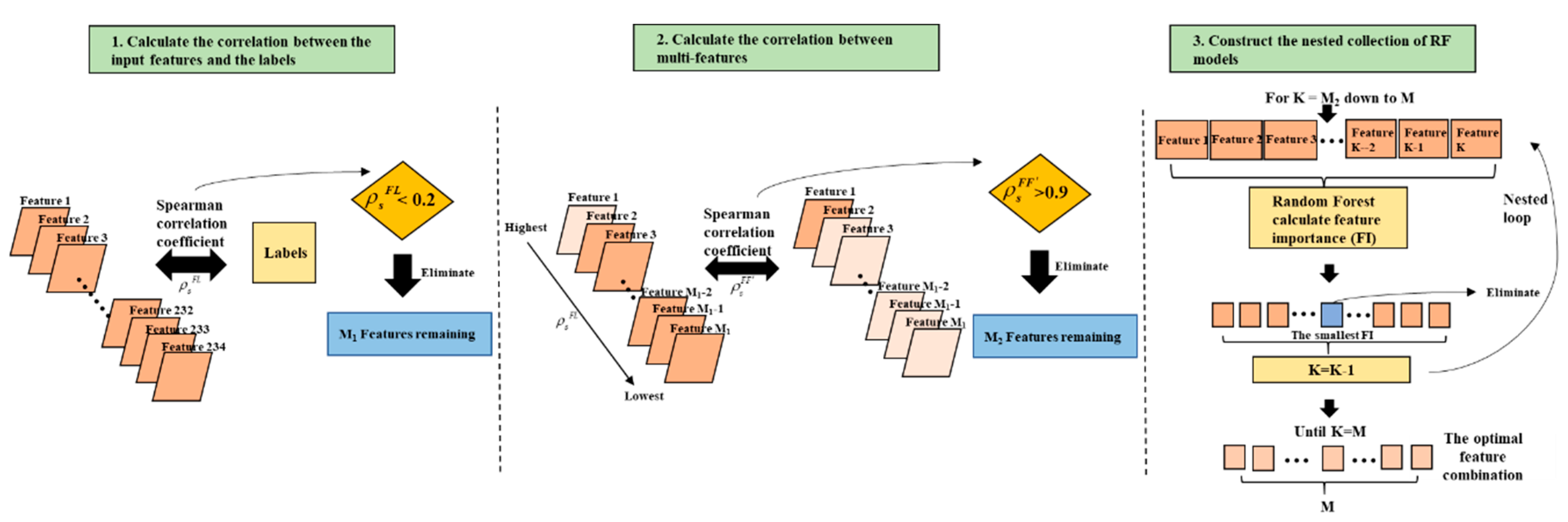
- One of the main innovations of this paper is OFSM, which is different from traditional feature selection methods, including filter, embedded, wrapper, and hybrid. The filter selection method selects features regardless of the model used and is commonly robust in overfitting and effective in computation time. The wrapper method performs evaluation on multiple subsets of the features and chooses the best subset of features that gives the highest accuracy to the model. Since the classifier needs to be trained multiple times, the computation time using the wrapper method (e.g., RFE) is usually much larger than that using the filter method. The embedded method (e.g., RF and XGBoost) can interact with the classifier and is less computationally intensive than the wrapper method, but it ignores the correlation between multiple features. OFSM is a hybrid method of filter, embedded, and wrapper, and has advantages in processing time and recognition accuracy. Considering the correlation between the multi-features and the processing time during the feature selection process, the features selected by OFSM are independent of each other and the time required for processing is acceptable. The experimental results demonstrate that OFSM performs optimally and the accuracy of the selected features for crop classification is higher than that of the original image directly sent to the classifier. Thus, we show that the preprocessing of feature selection is critical prior to classification.
- (2)
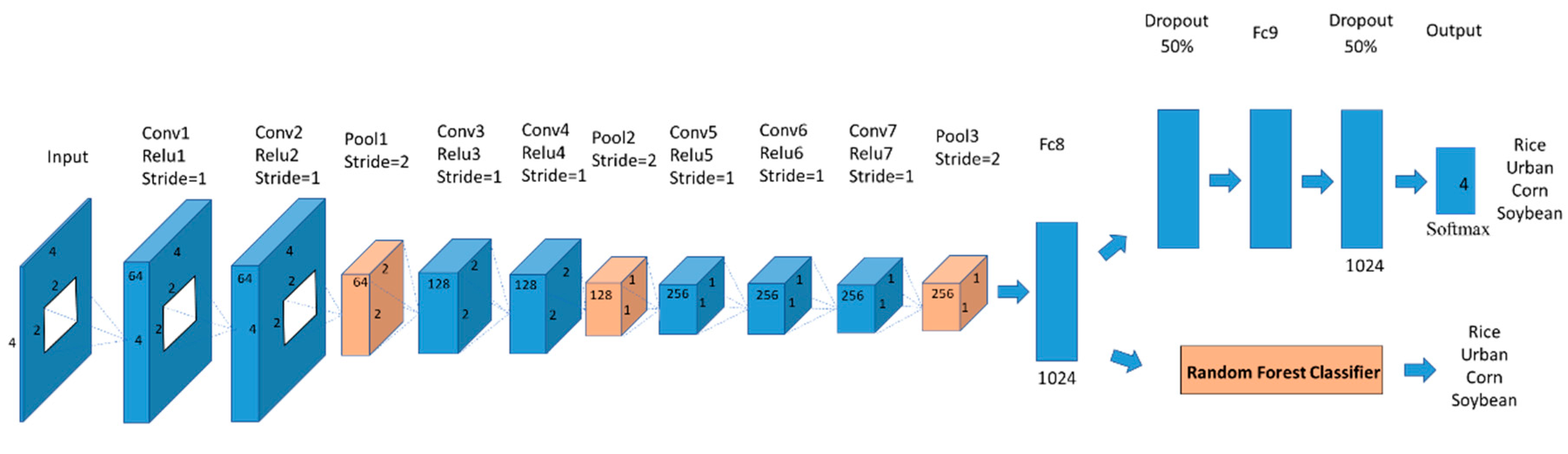
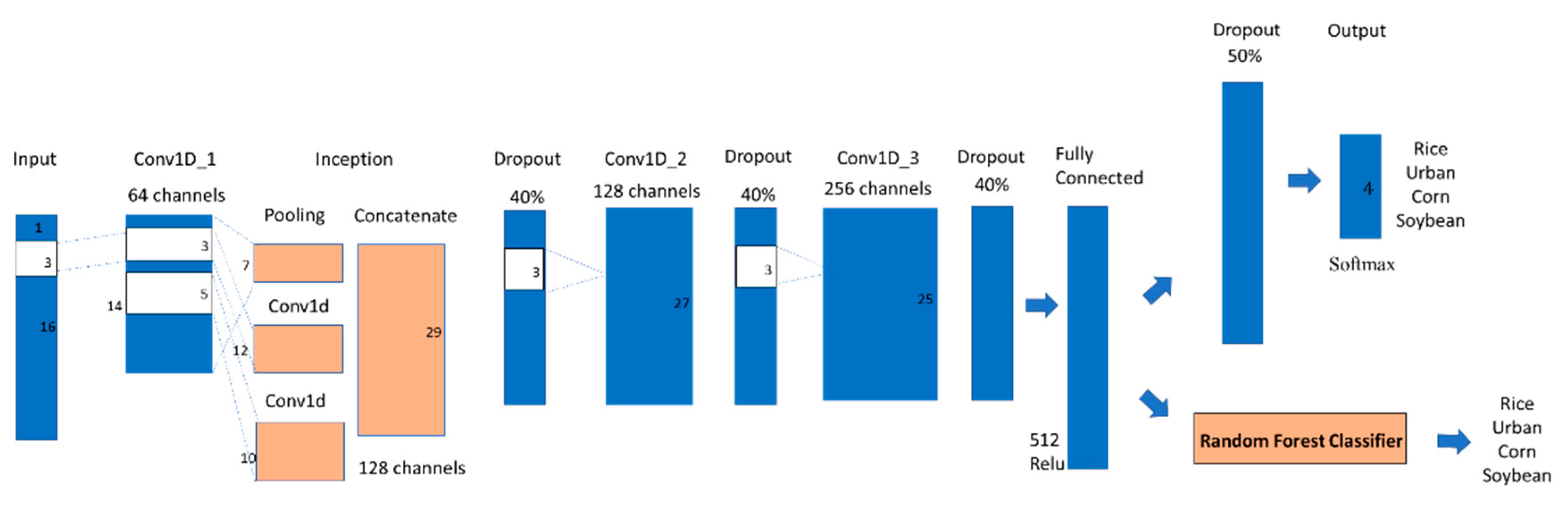
- Considering the advantages of multiple classifiers, we propose two hybrid CNN-RF networks to integrate the advantages of Conv1D and Visual Geometry Group (VGG) with RF, respectively. A traditional CNN uses an FC layer to make the final classification decision, and there is usually overfitting, especially with inadequate samples, which is not sufficiently robust and is computationally intensive. The use of RF instead of the FC layer to make the final decision can effectively alleviate the occurrence of overfitting. At the same time, we are committed to providing a reasonable scheme for the selection of a CNN network structure in crop mapping based on multi-temporal remote sensing images, and selecting the optimal hyperparameters for the CNN network can further improve the identification accuracy of crops. The results demonstrate that the proposed hybrid networks can integrate the advantages of the two classifiers and achieve more optimal crop classification results than the original deep-learning networks. In particular, the combination of temporal feature representation network (Conv1D) and RF achieves the optimal crop classification results. Compared with the mainstream networks (e.g., LSTM-RF, ResNet, and U-Net), the proposed Conv1D-RF still obtains better crop recognition results, indicating that the Conv1D-RF framework can mine more effective and efficient time series representations and achieve more accurate identification results for crops in multi-temporal classification tasks.
2. Data Resources
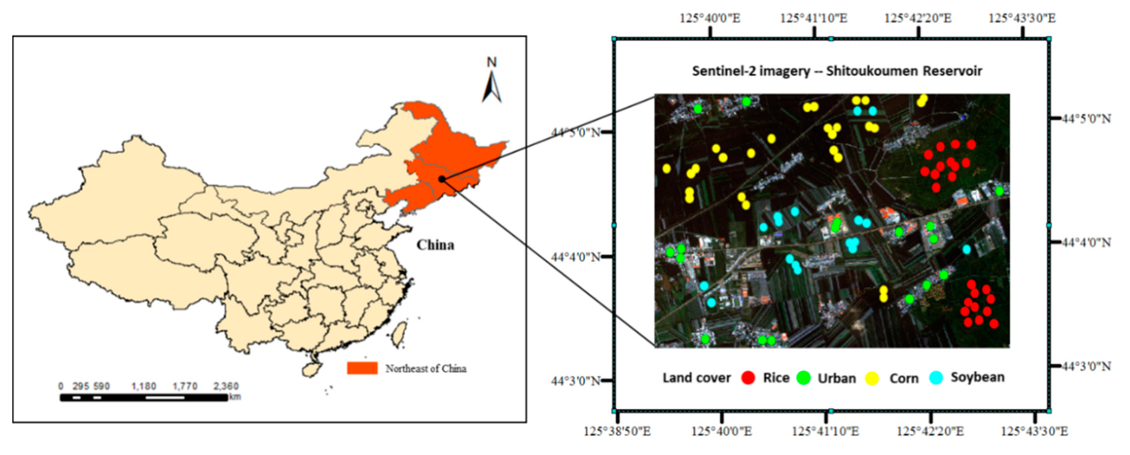
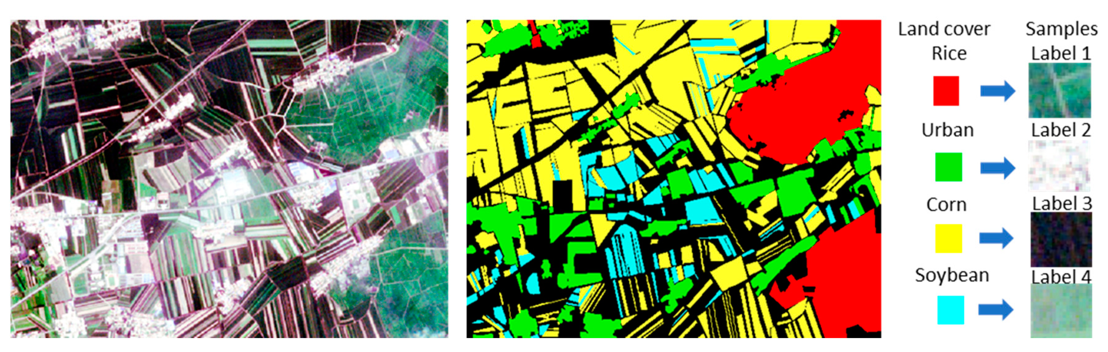
2.1. Study Area
2.2. Data
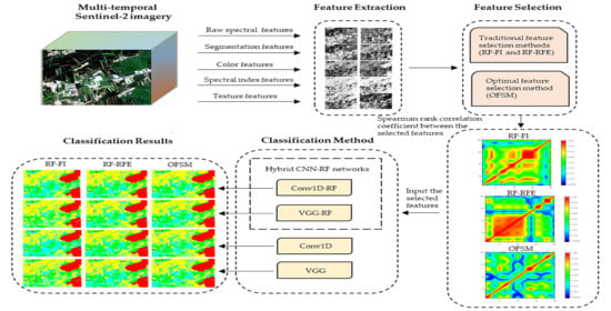
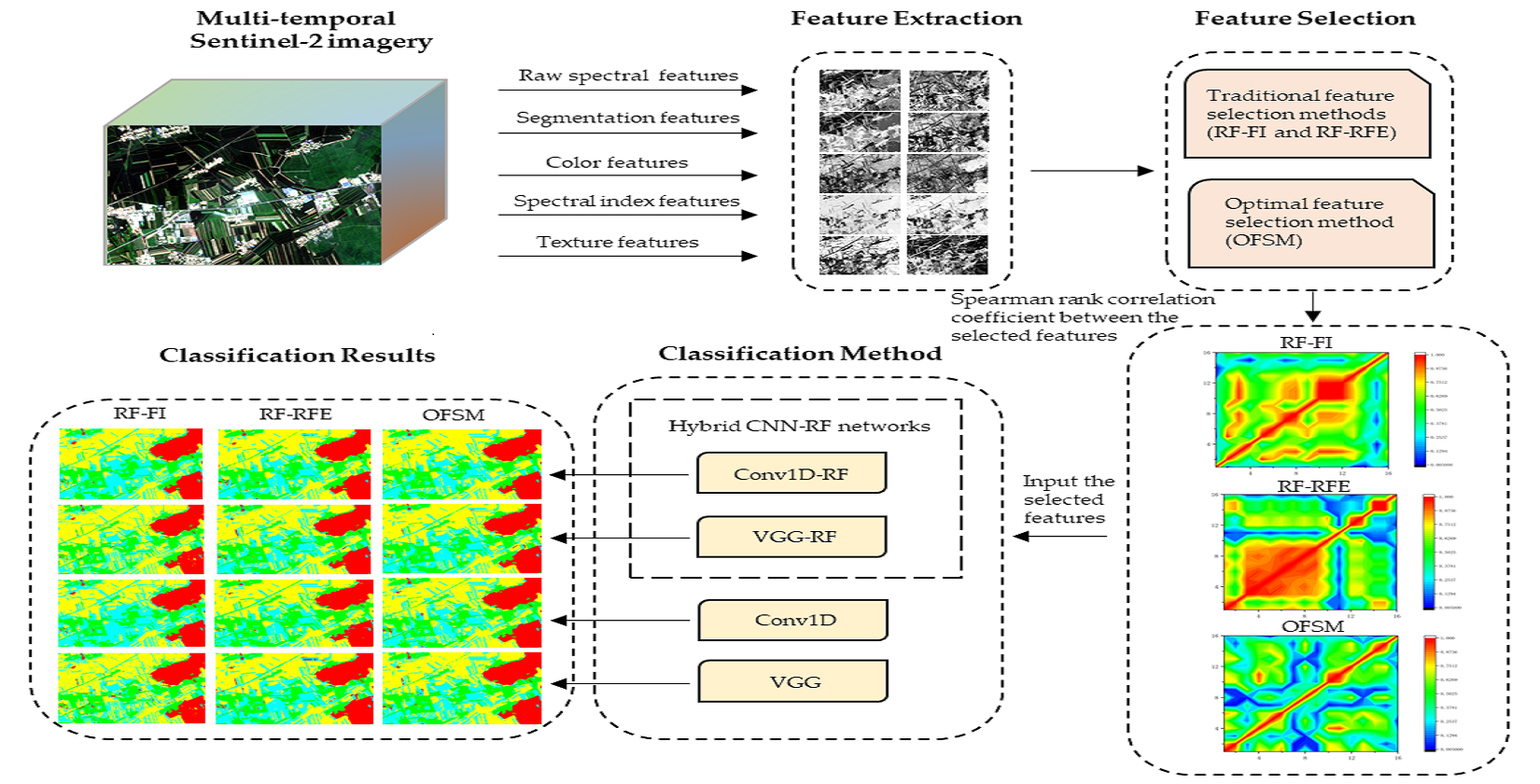
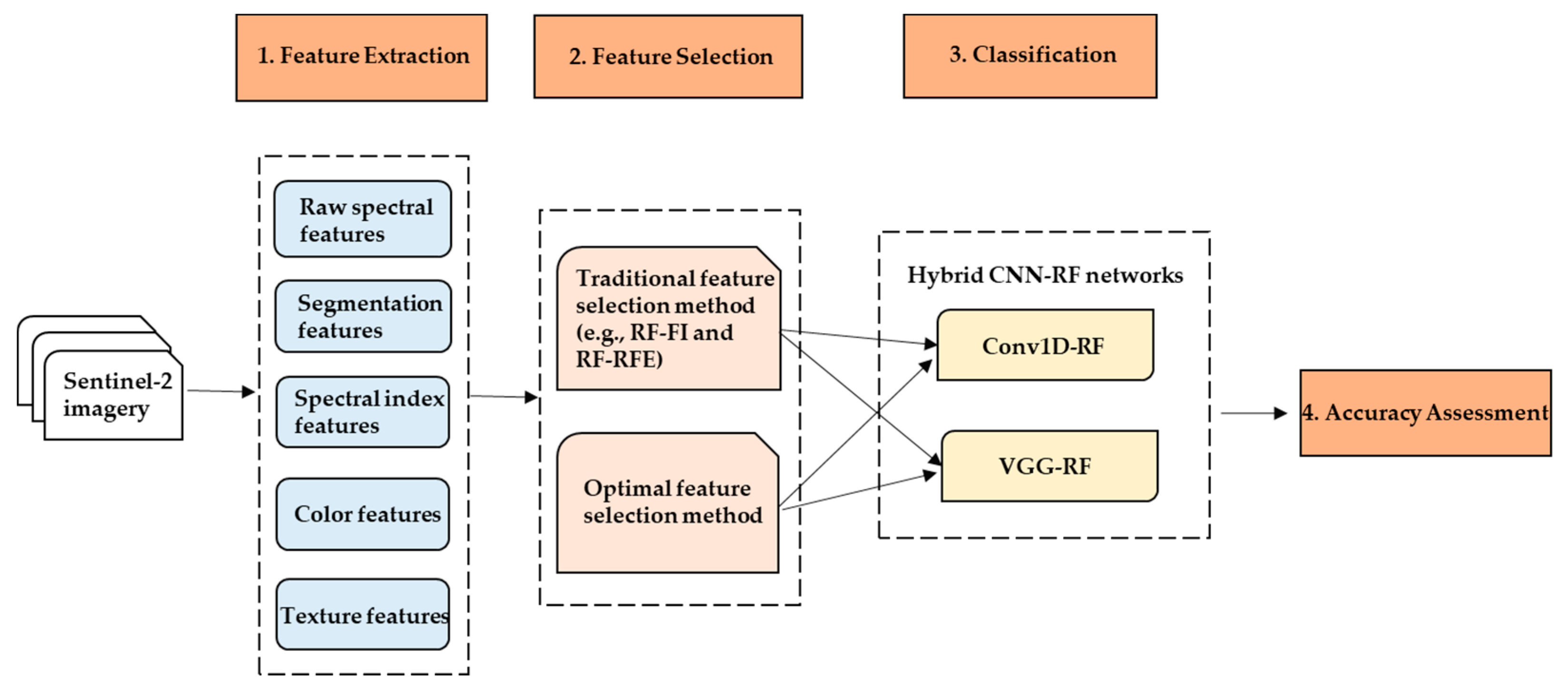
3. Methodology
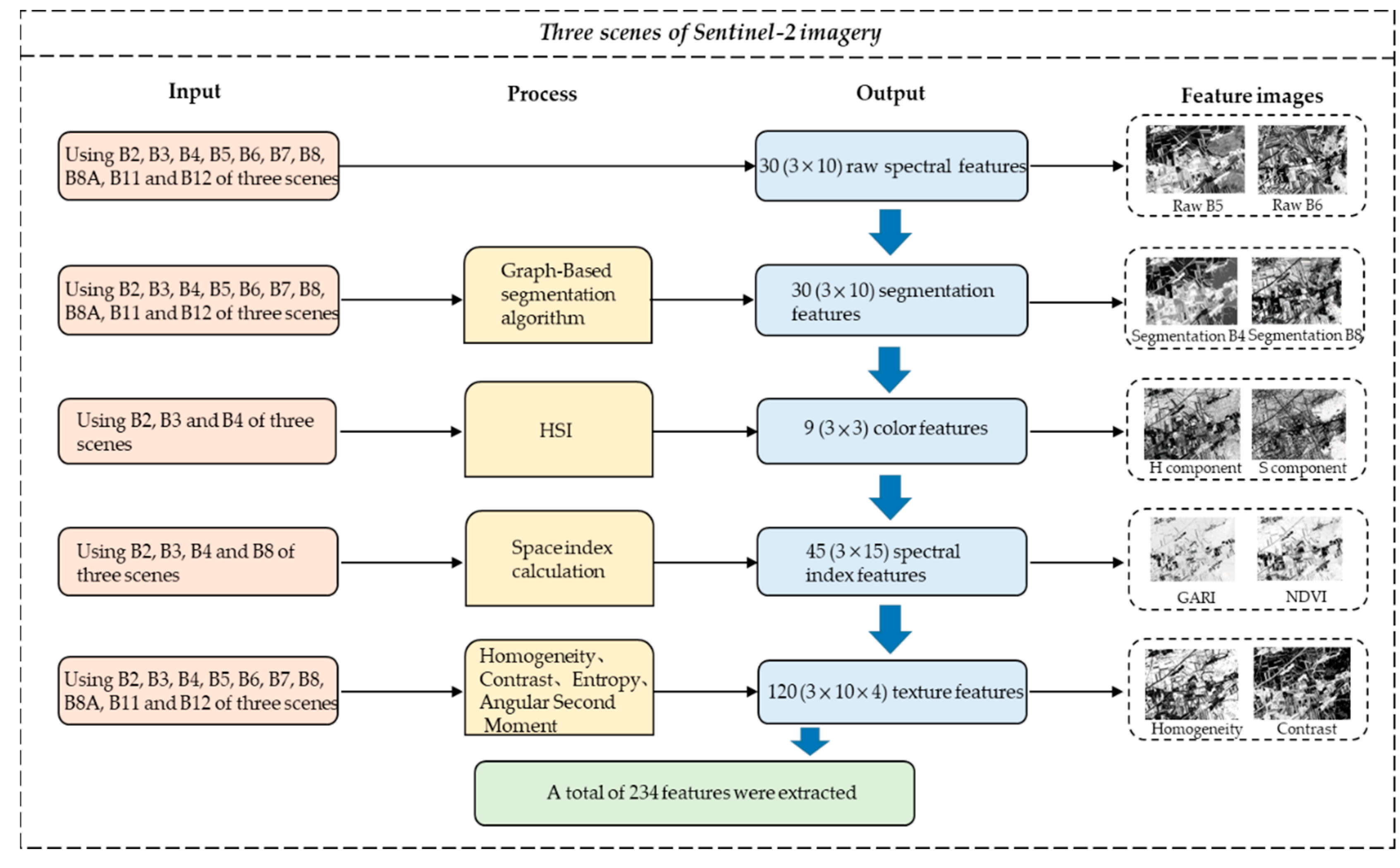
3.1. Feature Extraction
3.2. Feature Selection
3.2.1. Traditional Feature Selection Methods (TFSM)
3.2.2. Optimal Feature Selection Method (OFSM)
3.3. Deep-Learning Classification
3.3.1. Visual Geometry Group Combined with Random Forest (VGG-RF)
3.3.2. One-Dimensional Convolution Combined with Random Forest (Conv1D-RF)
3.4. Evaluation
4. Result
4.1. Feature Selection Comparison
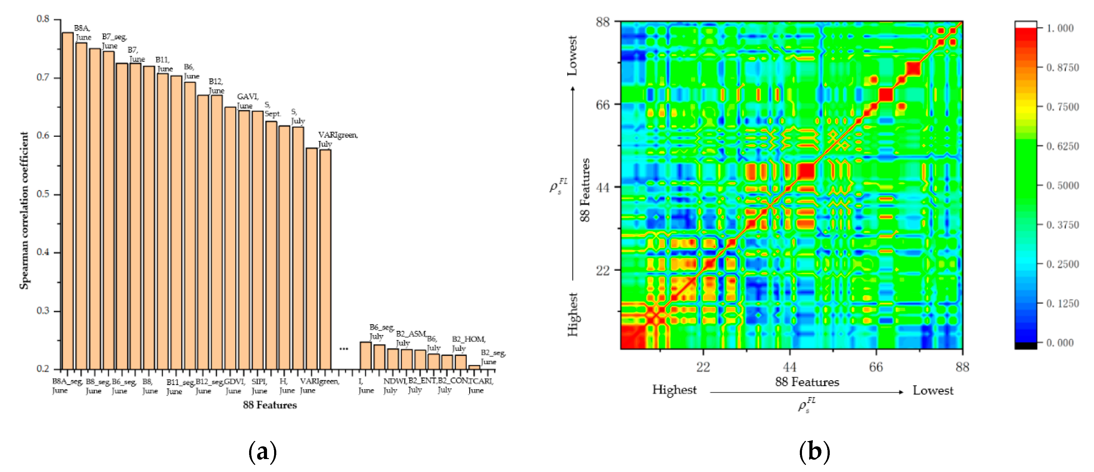
4.1.1. Features from OFSM
4.1.2. Methods Comparison
4.2. Deep-Learning Network Hyperparameter Selection
4.3. Classification and Accuracy Assessment
4.3.1. Comparison of the Hybrid CNN-RF Networks with the Original Deep-Learning Networks
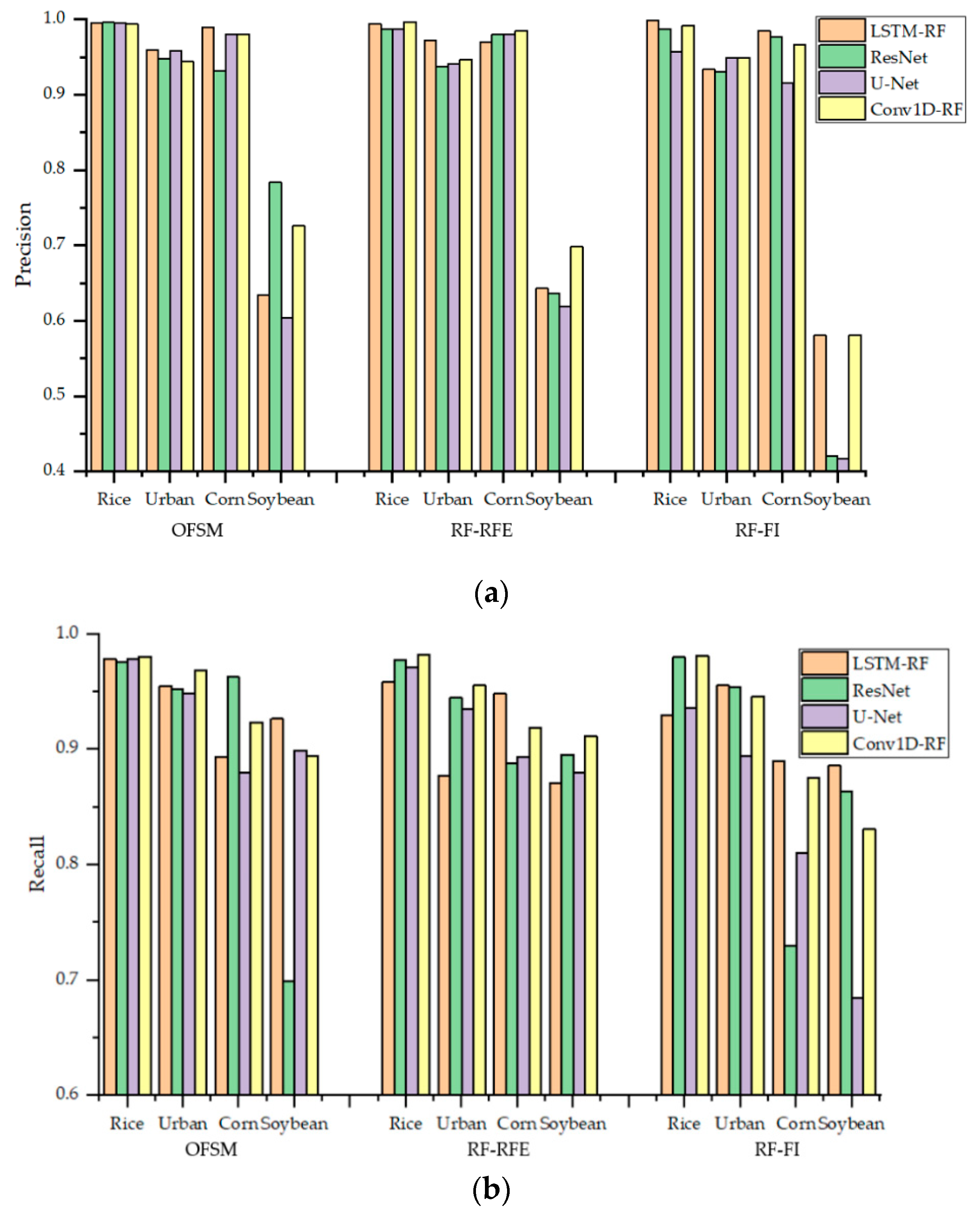
4.3.2. Comparison of Conv1D-RF with Mainstream Networks
5. Discussion
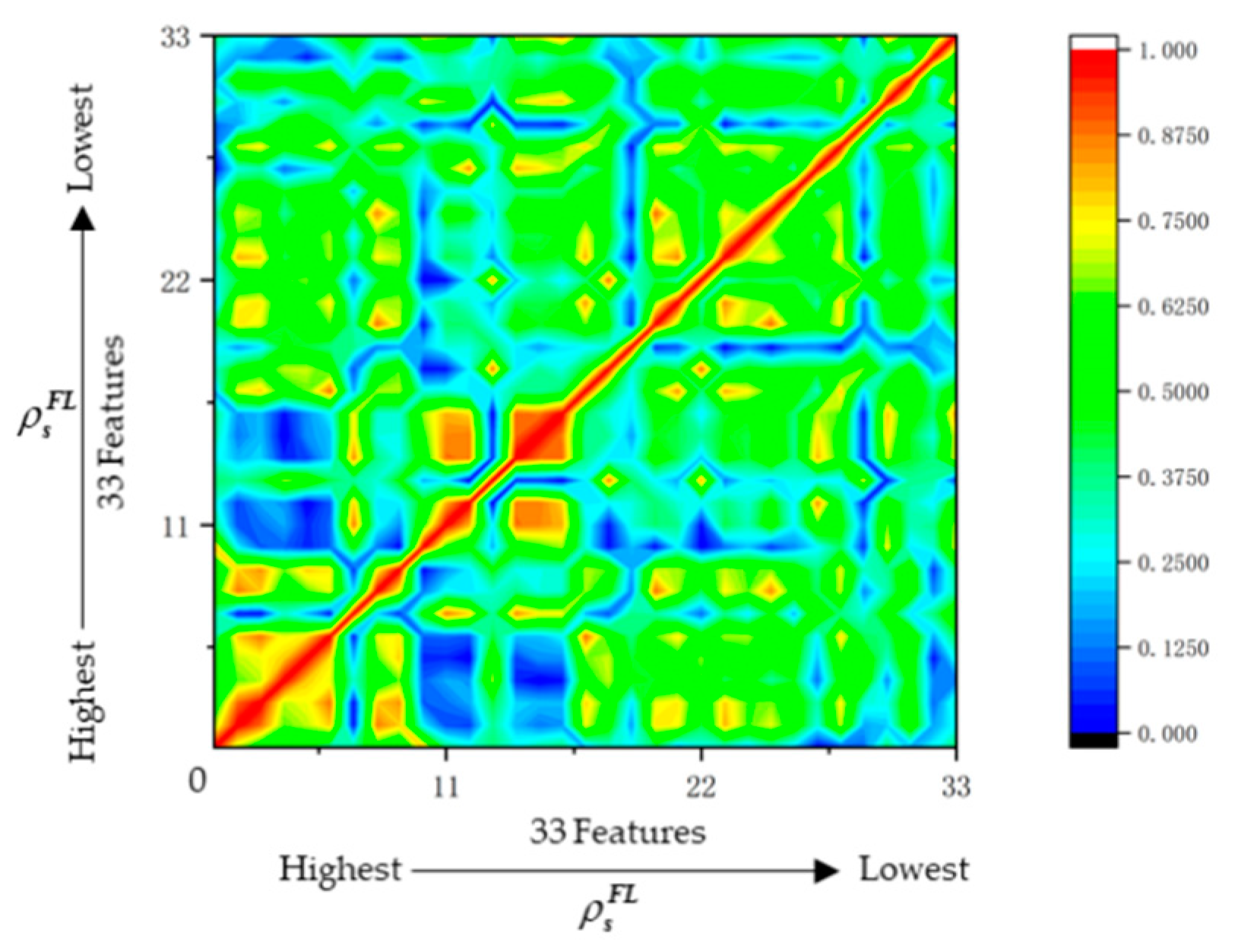
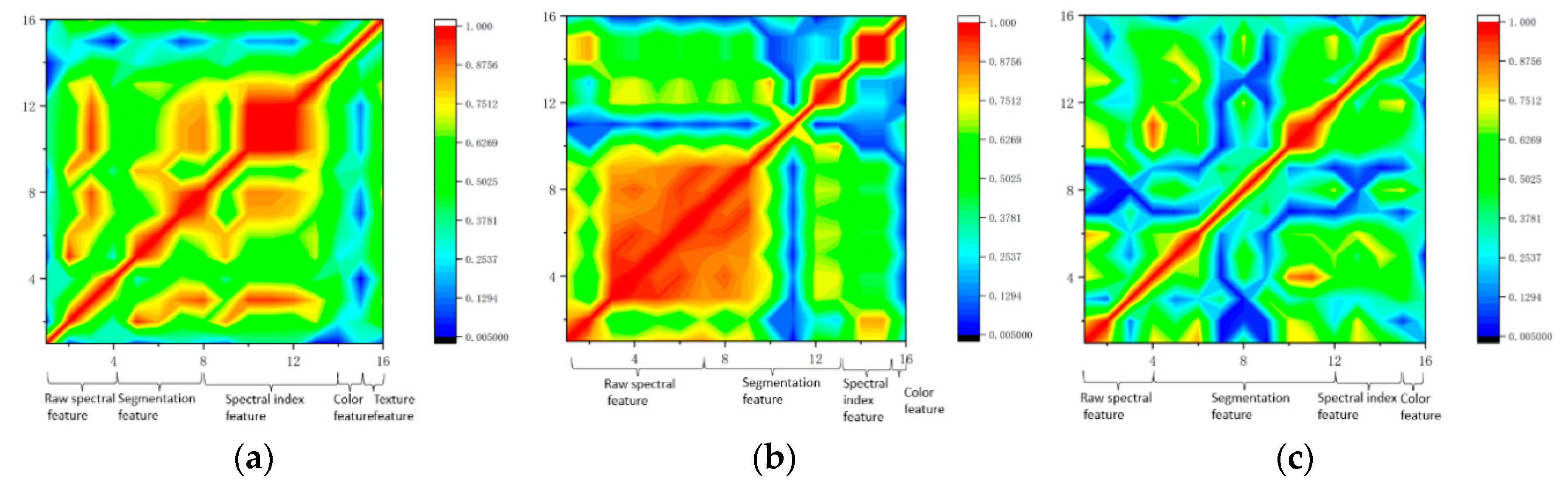
5.1. Analysis of Feature Selection Using OFSM
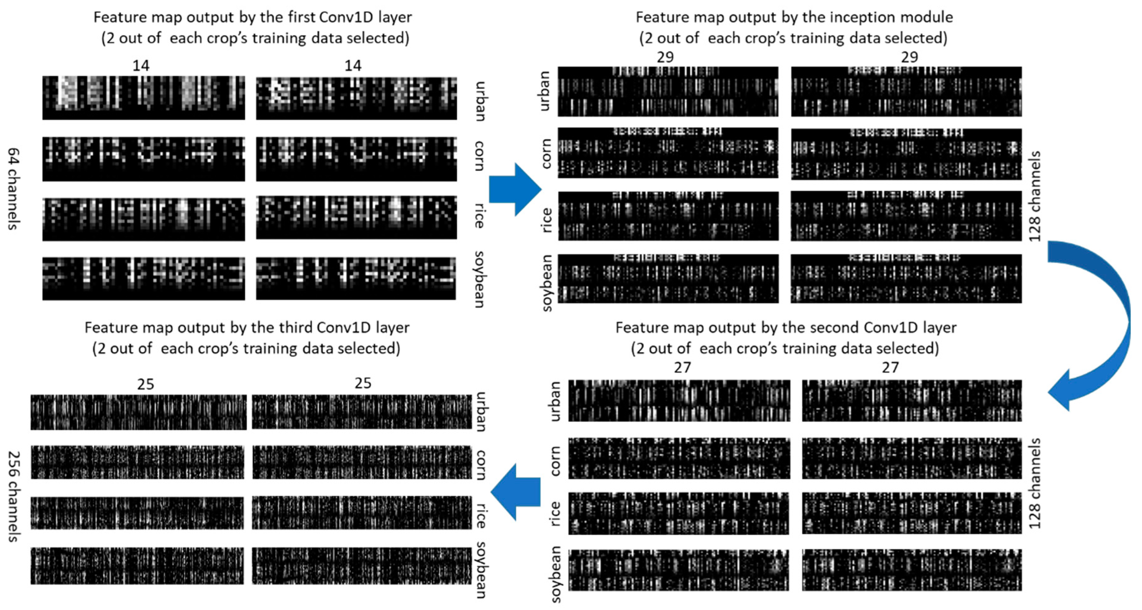
5.2. Conv1D Feature Map Visualization
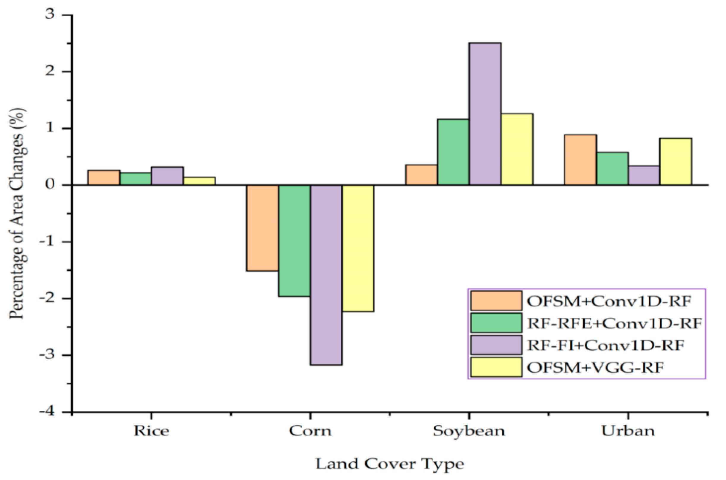
5.3. Crop Distribution Analysis
6. Conclusions
Author Contributions
Funding
Acknowledgments
Conflicts of Interest
References
- Bolton, D.K.; Friedl, M.A. Forecasting crop yield using remotely sensed vegetation indices and crop phenology metrics. Agric. For. Meteorol. 2013, 173, 74–84. [Google Scholar] [CrossRef]
- Cai, Y.; Guan, K.; Peng, J.; Wang, S.; Seifert, C.; Wardlow, B.; Li, Z. A high-performance and in-season classification system of field-level crop types using time-series Landsat data and a machine learning approach. Remote Sens. Environ. 2018, 210, 35–47. [Google Scholar] [CrossRef]
- Ji, S.; Zhang, C.; Xu, A.; Shi, Y.; Duan, Y. 3D convolutional neural networks for crop classification with multi-temporal remote sensing images. Remote Sens. 2018, 10, 75. [Google Scholar] [CrossRef]
- Wardlow, B.D.; Egbert, S.L.; Kastens, J.H. Analysis of time-series MODIS 250 m vegetation index data for crop classification in the US Central Great Plains. Remote Sens. Environ. 2007, 108, 2903–2910. [Google Scholar] [CrossRef]
- Chang, J.; Hansen, M.C.; Pittman, K.; Carroll, M.; DiMiceli, C. Corn and soybean mapping in the United States using MODIS time-series data sets. Agron. J. 2007, 99, 1654–1664. [Google Scholar] [CrossRef]
- Duro, D.C.; Franklin, S.E.; Dubé, M.G. Multi-scale object-based image analysis and feature selection of multi-sensor earth observation imagery using random forests. Int. J. Remote Sens. 2012, 33, 4502–4526. [Google Scholar] [CrossRef]
- Zheng, H.; Yuan, J.; Chen, L. Short-term load forecasting using EMD-LSTM neural networks with a Xgboost algorithm for feature importance evaluation. Energies 2017, 10, 1168. [Google Scholar] [CrossRef]
- Yan, K.; Zhang, D. Feature selection and analysis on correlated gas sensor data with recursive feature elimination. Sens. Actuators B Chem. 2015, 212, 353–363. [Google Scholar] [CrossRef]
- Hao, P.; Zhan, Y.; Wang, L.; Niu, Z.; Shakir, M. Feature selection of time series MODIS data for early crop classification using random forest: A case study in Kansas, USA. Remote Sens. 2015, 7, 5347–5369. [Google Scholar] [CrossRef]
- Yin, L.; You, N.; Zhang, G.; Huang, J.; Dong, J. Optimizing Feature Selection of Individual Crop Types for Improved Crop Mapping. Remote Sens. 2020, 12, 162. [Google Scholar] [CrossRef]
- Liu, H.; An, H. Preliminary tests on the performance of MLC-RFE and SVM-RFE in Lansat-8 image classification. Arab. J. Geosci. 2020, 13, 130. [Google Scholar] [CrossRef]
- Mathur, A.; Foody, G.M. Crop classification by support vector machine with intelligently selected training data for an operational application. Int. J. Remote Sens. 2008, 29, 2227–2240. [Google Scholar] [CrossRef]
- Ahmad, I.; Siddiqi, M.H.; Fatima, I.; Lee, S.; Lee, Y.K. Weed classification based on Haar wavelet transform via k-nearest neighbor (k-NN) for real-time automatic sprayer control system. In Proceedings of the 5th International Conference on Ubiquitous Information Management and Communication, Seoul, Korea, 21–23 February 2011; p. 17. [Google Scholar]
- Murthy, C.; Raju, P.; Badrinath, K. Classification of wheat crop with multi-temporal images: Performance of maximum likelihood and artificial neural networks. Int. J. Remote Sens. 2003, 24, 4871–4890. [Google Scholar] [CrossRef]
- Chen, T.; He, T.; Benesty, M.; Khotilovich, V.; Tang, Y. Xgboost: Extreme Gradient Boosting. R Package Version 0.6-4. Available online: Cran.fhcrc.org/web/packages/xgboost/vignettes/xgboost.pdf (accessed on 1 January 2017).
- Friedl, M.A.; Brodley, C.E. Decision tree classification of land cover from remotely sensed data. Remote Sens. Environ. 1997, 61, 399–409. [Google Scholar] [CrossRef]
- Tatsumi, K.; Yamashiki, Y.; Torres, M.C.; Taipe, C.R. Crop classification of upland fields using Random forest of time-series Landsat 7 ETM+ data. Comput. Electron. Agric. 2015, 115, 171–179. [Google Scholar] [CrossRef]
- Kumar, P.; Gupta, D.K.; Mishra, V.N.; Prasad, R. Comparison of support vector machine, artificial neural network, and spectral angle mapper algorithms for crop classification using LISS IV data. Int. J. Remote Sens. 2015, 36, 1604–1617. [Google Scholar] [CrossRef]
- Li, H.; Zhang, C.; Zhang, S.; Atkinson, P.M. Crop classification from full-year fully-polarimetric L-band UAVSAR time-series using the Random Forest algorithm. Int. J. Appl. Earth Obs. 2020, 87, 102032. [Google Scholar] [CrossRef]
- Zhang, H.; Eziz, A.; Xiao, J.; Tao, S.; Wang, S.; Tang, Z.; Fang, J. High-Resolution Vegetation Mapping Using Extreme Gradient Boosting Based on Extensive Features. Remote Sens. 2019, 11, 1505. [Google Scholar] [CrossRef]
- Romero, A.; Gatta, C.; Camps-Valls, G. Unsupervised deep feature extraction for remote sensing image classification. IEEE Trans. Geosci. Remote Sens. 2016, 54, 1349–1362. [Google Scholar] [CrossRef]
- Castelluccio, M.; Poggi, G.; Sansone, C.; Verdoliva, L. Land Use Classification in Remote Sensing Images by Convolutional Neural Networks. Available online: http://arxiv.org/abs/1508.00092 (accessed on 14 August 2015).
- Xu, X.; Li, W.; Ran, Q. Multisource remote sensing data classification based on convolutional neural network. IEEE Trans. Geosci. Remote Sens. 2018, 56, 937–949. [Google Scholar] [CrossRef]
- Rußwurm, M.; Körner, M. Multi-Temporal Land Cover Classification with Long Short-Term Memory Neural Networks. Int. Arch. Photogramm. Remote Sens. Spat. Inf. Sci. 2017, 42, 551. [Google Scholar] [CrossRef]
- Rußwurm, M.; Körner, M. Temporal Vegetation Modelling Using Long Short-Term Memory Networks for Crop Identification from Medium-Resolution Multi-spectral Satellite Images. In Proceedings of the IEEE Computer Society Conference on Computer Vision and Pattern Recognition Workshops, Honolulu, HI, USA, 21–26 July 2017; pp. 1496–1504. [Google Scholar]
- Zhong, L.; Hu, L.; Zhou, H. Deep learning based multi-temporal crop classification. Remote Sens. Environ. 2019, 221, 430–443. [Google Scholar] [CrossRef]
- Guidici, D.; Clark, M. One-Dimensional convolutional neural network land-cover classification of multi-seasonal hyperspectral imagery in the San Francisco Bay Area, California. Remote Sens. 2017, 9, 629. [Google Scholar] [CrossRef]
- Ko, A.H.R.; Sabourin, R. Single Classifier-based Multiple Classification Scheme for weak classifiers: An experimental comparison. Expert Syst. Appl. 2013, 40, 3606–3622. [Google Scholar] [CrossRef]
- Debeir, O.; Van Den Steen, I.; Latinne, P.; Van Ham, P.; Wolff, E. Textural and contextual land-cover classification using single and multiple classifier systems. Photogramm. Eng. Remote Sens. 2002, 68, 597–606. [Google Scholar]
- Briem, G.J.; Benediktsson, J.A.; Sveinsson, J.R. Multiple classifiers applied to multisource remote sensing data. IEEE Trans. Geosci. Remote Sens. 2002, 40, 2291–2299. [Google Scholar] [CrossRef]
- Du, P.; Xia, J.; Zhang, W.; Tan, K.; Liu, Y.; Liu, S. Multiple classifier system for remote sensing image classification: A review. Sensors 2012, 12, 4764–4792. [Google Scholar] [CrossRef]
- Zhou, Z.H. Ensemble learning. In Encyclopedia of Biometrics; Springer: Berlin/Heidelberg, Germany, 2015; pp. 411–416. [Google Scholar]
- Leng, J.; Li, T.; Bai, G.; Dong, Q.; Dong, H. Cube-CNN-SVM: A novel hyperspectral image classification method. In Proceedings of the 2016 IEEE 28th International Conference on Tools with Artificial Intelligence (ICTAI), San Jose, CA, USA, 6–8 November 2016; pp. 1027–1034. [Google Scholar]
- Immitzer, M.; Vuolo, F.; Atzberger, C. First Experience with Sentinel-2 Data for Crop and Tree Species Classifications in Central Europe. Remote Sens. 2016, 8, 166. [Google Scholar] [CrossRef]
- Vuolo, F.; Neuwirth, M.; Immitzer, M.; Atzberger, C.; Ng, W.T. How much does multi-temporal Sentinel-2 data improve crop type classification? Int. J. Appl. Earth Obs. Geoinf. 2018, 72, 122–130. [Google Scholar] [CrossRef]
- Sharma, V.; Irmak, S.; Kilic, A.; Sharma, V.; Gilley, J.E.; Meyer, G.E.; Marx, D. Quantification and mapping of surface residue cover for maize and soybean fields in south central Nebraska. Trans. ASABE 2016, 59, 925–939. [Google Scholar]
- Felzenszwalb, P.F.; Huttenlocher, D.P. Efficient graph-based image segmentation. Int. J. Comput. Vis. 2004, 59, 167–181. [Google Scholar] [CrossRef]
- Connolly, C.; Fleiss, T. A study of efficiency and accuracy in the transformation from RGB to CIELAB color space. IEEE Trans. Image Process. 1997, 6, 1046–1048. [Google Scholar] [CrossRef] [PubMed]
- Peña-Barragán, J.M.; Ngugi, M.K.; Plant, R.E.; Six, J. Object-based crop identification using multiple vegetation indices, textural features and crop phenology. Remote Sens. Environ. 2011, 115, 1301–1316. [Google Scholar] [CrossRef]
- Ruiz, L.A.; Fdez-sarría, A.; Recio, J.A. Texture feature extraction for classification of remote sensing data using wavelet decomposition: A comparative study. Int. Arch. Photogramm. Remote Sens. 2004, XXXV, 1682–1750. [Google Scholar]
- Genuer, R.; Poggi, J.M.; Tuleau-Malot, C. VSURF: An R Package for variable selection using random forests. R J. 2015, 7, 19–33. [Google Scholar] [CrossRef]
- Granitto, P.M.; Furlanello, C.; Biasioli, F.; Gasperi, F. Recursive feature elimination with random forest for PTR-MS analysis of agroindustrial products. Chemom. Intell. Lab. Syst. 2006, 83, 83–90. [Google Scholar] [CrossRef]
- Zar, J.H. Significance testing of the spearman rank correlation coefficient. J. Am. Stat. Assoc. 1972, 67, 578–580. [Google Scholar] [CrossRef]
- Khare, S.; Bhandari, A.; Singh, S.; Arora, A. ECG arrhythmia classification using spearman rank correlation and support vector machine. In Proceedings of the International Conference on Soft Computing for Problem Solving (SocProS 2011), Roorkee, India, 20–22 December 2011; pp. 591–598. [Google Scholar]
- Sengupta, A.; Ye, Y.; Wang, R.; Liu, C.; Roy, K. Going deeper in spiking neural networks: VGG and residual architectures. Front. Neurosci. 2019, 13. [Google Scholar] [CrossRef]
- Mateen, M.; Wen, J.; Song, S.; Huang, Z. Fundus image classification using VGG-19 architecture with PCA and SVD. Symmetry 2019, 11, 1. [Google Scholar] [CrossRef]
- Dong, L.; Du, H.; Mao, F.; Han, N.; Li, X.; Zhou, G.; Liu, T. Very High Resolution Remote Sensing Imagery Classification Using a Fusion of Random Forest and Deep Learning Technique—Subtropical Area for Example. IEEE J. Sel. Top. Appl. Earth Obs. Remote Sens. 2019, 13, 113–128. [Google Scholar] [CrossRef]
- Fu, G.; Liu, C.; Zhou, R.; Sun, T.; Zhang, Q. Classification for high resolution remote sensing imagery using a fully convolutional network. Remote Sens. 2017, 9, 498. [Google Scholar] [CrossRef]
- Punia, S.; Nikolopoulos, K.; Singh, S.P.; Madaan, J.K.; Litsiou, K. Deep learning with long short-term memory networks and random forests for demand forecasting in multi-channel retail. Int. J. Prod. Res. 2020, 1–16. [Google Scholar] [CrossRef]
- Liu, S.; Tian, G.; Xu, Y. A novel scene classification model combining ResNet based transfer learning and data augmentation with a filter. Neurocomputing 2019, 338, 191–206. [Google Scholar] [CrossRef]
- Rakhlin, A.; Davydow, A.; Nikolenko, S. Land Cover Classification from Satellite Imagery with U-Net and Lovasz-Softmax Loss. In Proceedings of the IEEE Conference on Computer Vision and Pattern Recognition (CVPR) Workshops, Salt Lake City, UT, USA, 18–22 June 2018. [Google Scholar]
- Kussul, N.; Lavreniuk, M.; Skakun, S.; Shelestov, A. Deep learning classification of land cover and crop types using remote sensing data. IEEE Geosci. Remote Sens. Lett. 2017, 14, 778–782. [Google Scholar] [CrossRef]
- Zhong, L.; Hu, L.; Yu, L.; Gong, P.; Biging, G.S. Automated mapping of soybean and corn using phenology. ISPRS J. Photogramm. Remote Sens. 2016, 119, 151–164. [Google Scholar] [CrossRef]
- Zhong, L.; Gong, P.; Biging, G.S. Efficient corn and soybean mapping with temporal extendability: A multi-year experiment using Landsat imagery. Remote Sens. Environ. 2014, 140, 1–13. [Google Scholar] [CrossRef]


| ID | 1 | 2 | 3 | 4 | Total |
|---|---|---|---|---|---|
| Type | Rice | Urban | Corn | Soybean | |
| Number | 23 | 17 | 26 | 17 | 83 |
| Band Name | Central Wavelength (um) | Resolution (m) |
|---|---|---|
| B1-Coastal aerosol | 0.443 | 60 |
| B2-Blue | 0.49 | 10 |
| B3-Green | 0.56 | 10 |
| B4-Red | 0.665 | 10 |
| B5-Vegetation Red Edge | 0.705 | 20 |
| B6-Vegetation Red Edge | 0.74 | 20 |
| B7-Vegetation Red Edge | 0.783 | 20 |
| B8-NIR | 0.842 | 10 |
| B8A-Vegetation Red Edge | 0.865 | 20 |
| B9-Water vapor | 0.945 | 60 |
| B10-SWIR-Cirrus | 1.375 | 60 |
| B11-SWIR | 1.61 | 20 |
| B12-SWIR | 2.19 | 20 |
| Spectral Index | Calculation Formula |
|---|---|
| NDVI | |
| DVI | |
| RDVI | |
| NDWI | |
| RVI | |
| EVI | |
| TVI | |
| TCARI | |
| GI | |
| VIgreen | |
| VARIgreen | |
| GARI | |
| GDVI | |
| SAVI | |
| SIPI |
| Texture Features | Statistical Characteristics |
|---|---|
| Homogeneity: | Measure local homogeneity |
| Contrast: | Measure the difference between the maximum and minimum values in the neighborhood |
| Entropy: | Measuring image disorder |
| Angular Second Moment: | Describe local stationarity |
| Raw Spectral Feature | Segmentation Feature | Spectral Index Feature | Color Feature |
|---|---|---|---|
| B5 and B11, June; B5 and B12, September | B2, B4 and B5, June; B6, July; B2, B5, B6 and B12, September | GARI, June; NDWI and VARIgreen, July | Saturation, September |
| Method | RF-FI | RF-RFE | OFSM |
|---|---|---|---|
| Time Consumption | 1.97 s | 132.54 s | 26.05 s |
| Software: Anaconda3-2018.12 Python 3.7.1 Computer configuration: Windows 10 x64, i5-8300H CPU @ 2.30GHz, 8G RAM | |||
| Hyperparameter Name (Description) | Tested Values | Optimal Values | ||
|---|---|---|---|---|
| VGG-RF | Conv1D-RF | VGG-RF | Conv1D-RF | |
| num_filter1 (number of filters in the first convolutional layer) | 32, 64, 128 | 32, 64, 128 | 64 | 64 |
| convolution kernel_size (the filter size of convolutional layers) | 2 × 2, 3 × 3 | 3, 5, 7/3, 5, 7 | 2 × 2 | 3/5 |
| pooling kernel_size (the filter size of pooling layers) | 2 × 2, 3 × 3 | 2, 3, 4 | 2 × 2 | 2 |
| learning_rate (learning rate) | 0.1, 0.01, 0.001 | 0.1, 0.01, 0.001 | 0.001 | 0.001 |
| dropout (dropout rate in hidden layers) | 40%, 50%, 60%, 70%, 80% | 40%, 50%, 60%, 70%, 80%/40%, 50%, 60%, 70%, 80% | 50% | 40%/50% |
| max_iterations (maximum number of iterations) | 5000, 10000, 15000 | 5000, 10000, 15000 | 10000 | 5000 |
| batch_size (number of samples for each training) | 50, 60, 80, 100 | 50, 60, 80, 100 | 80 | 80 |
| Conv1D-RF | VGG-RF | Conv1D | VGG | |
|---|---|---|---|---|
| RF-FI |  |  |  |  |
| RF-RFE |  |  |  |  |
| OFSM |  |  |  |  |
 | ||||
| Method | OA/K Coefficient | |||
|---|---|---|---|---|
| Conv1D-RF | VGG-RF | Conv1D | VGG | |
| RF-FI | 90.97%/0.871 | 90.13%/0.853 | 87.47%/0.824 | 86.74%/0.814 |
| RF-RFE | 94.01%/0.914 | 92.81%/0.897 | 92.33%/0.890 | 91.58%/0.880 |
| OFSM | 94.27%/0.917 | 93.23%/0.903 | 92.59%/0.894 | 91.89%/0.884 |
| Method | OA/K Coefficient | |||
|---|---|---|---|---|
| Conv1D-RF | LSTM-RF | ResNet | U-Net | |
| RF-FI | 90.97%/0.871 | 91.16%/0.874 | 84.76%/0.789 | 84.33%/0.777 |
| RF-RFE | 94.01%/0.914 | 92.84%/0.896 | 92.14%/0.887 | 91.89%/0.884 |
| OFSM | 94.27%/0.917 | 92.91%/0.899 | 93.55%/0.905 | 91.92%/0.885 |
| Input Data | OA/Time Consumption | |
|---|---|---|
| Conv1D-RF | VGG-RF | |
| 16 feature bands | 94.27%/16′42″ | 93.23%/24′22″ |
| 30 raw spectral bands | 92.78%/40′54″ | 91.64%/58′15″ |
| Land Cover Type | Land Cover Area (ha)/Percentage of Area | ||||
|---|---|---|---|---|---|
| Reference Dataset | OFSM+ Conv1D-RF | RF-RFE+ Conv1D-RF | RF-FI+ Conv1D-RF | OFSM+ VGG-RF | |
| Rice | 473.15/23.40% | 478.60/23.67% | 477.80/23.63% | 479.82/23.73% | 476.18/23.55% |
| Corn | 905.86/44.80% | 874.52/43.25% | 865.42/42.80% | 840.95/41.59% | 859.96/42.53% |
| Soybean | 258.81/12.80% | 266.50/13.18% | 282.68/13.98% | 309.97/15.33% | 284.70/14.08% |
| Urban | 384.18/19.00% | 402.38/19.90% | 396.10/19.59% | 391.26/19.35% | 401.16/19.84% |
| Land Cover Type | Reference Dataset (Pixels) | Total | User’s Accuracy (%) | Commission (%) | |||
|---|---|---|---|---|---|---|---|
| Rice | Urban | Corn | Soybean | ||||
| Rice | 47,553 | 32 | 271 | 9 | 47,865 | 99.35 | 0.65 |
| Urban | 242 | 38,010 | 925 | 1078 | 40,255 | 94.42 | 5.58 |
| Corn | 257 | 267 | 85,688 | 1205 | 87,417 | 98.02 | 1.98 |
| Soybean | 454 | 939 | 5903 | 19,360 | 26,656 | 72.63 | 27.37 |
| Total | 48,506 | 39,248 | 92,787 | 21,652 | 202,193 | ||
| Producer’s Accuracy (%) | 98.03 | 96.84 | 92.35 | 89.41 | |||
| Omission (%) | 1.97 | 3.16 | 7.65 | 10.59 | |||
© 2020 by the authors. Licensee MDPI, Basel, Switzerland. This article is an open access article distributed under the terms and conditions of the Creative Commons Attribution (CC BY) license (http://creativecommons.org/licenses/by/4.0/).
Share and Cite
Yang, S.; Gu, L.; Li, X.; Jiang, T.; Ren, R. Crop Classification Method Based on Optimal Feature Selection and Hybrid CNN-RF Networks for Multi-Temporal Remote Sensing Imagery. Remote Sens. 2020, 12, 3119. https://doi.org/10.3390/rs12193119
Yang S, Gu L, Li X, Jiang T, Ren R. Crop Classification Method Based on Optimal Feature Selection and Hybrid CNN-RF Networks for Multi-Temporal Remote Sensing Imagery. Remote Sensing. 2020; 12(19):3119. https://doi.org/10.3390/rs12193119
Chicago/Turabian StyleYang, Shuting, Lingjia Gu, Xiaofeng Li, Tao Jiang, and Ruizhi Ren. 2020. "Crop Classification Method Based on Optimal Feature Selection and Hybrid CNN-RF Networks for Multi-Temporal Remote Sensing Imagery" Remote Sensing 12, no. 19: 3119. https://doi.org/10.3390/rs12193119
APA StyleYang, S., Gu, L., Li, X., Jiang, T., & Ren, R. (2020). Crop Classification Method Based on Optimal Feature Selection and Hybrid CNN-RF Networks for Multi-Temporal Remote Sensing Imagery. Remote Sensing, 12(19), 3119. https://doi.org/10.3390/rs12193119