Object-Based Approach Using Very High Spatial Resolution 16-Band WorldView-3 and LiDAR Data for Tree Species Classification in a Broadleaf Forest in Quebec, Canada


Abstract
1. Introduction
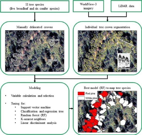
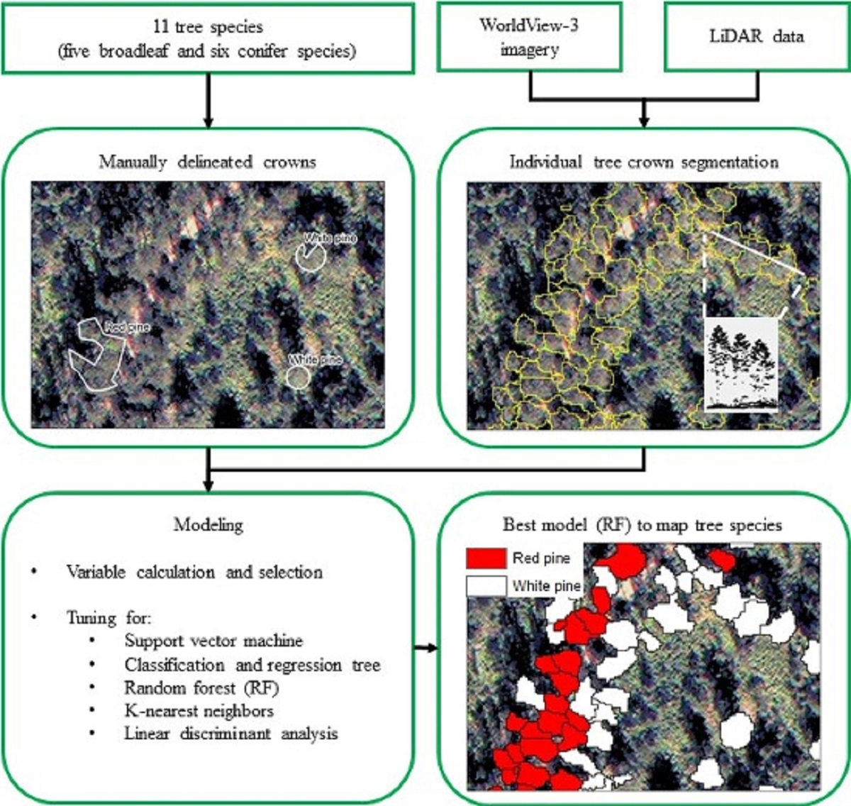
2. Data and Methods
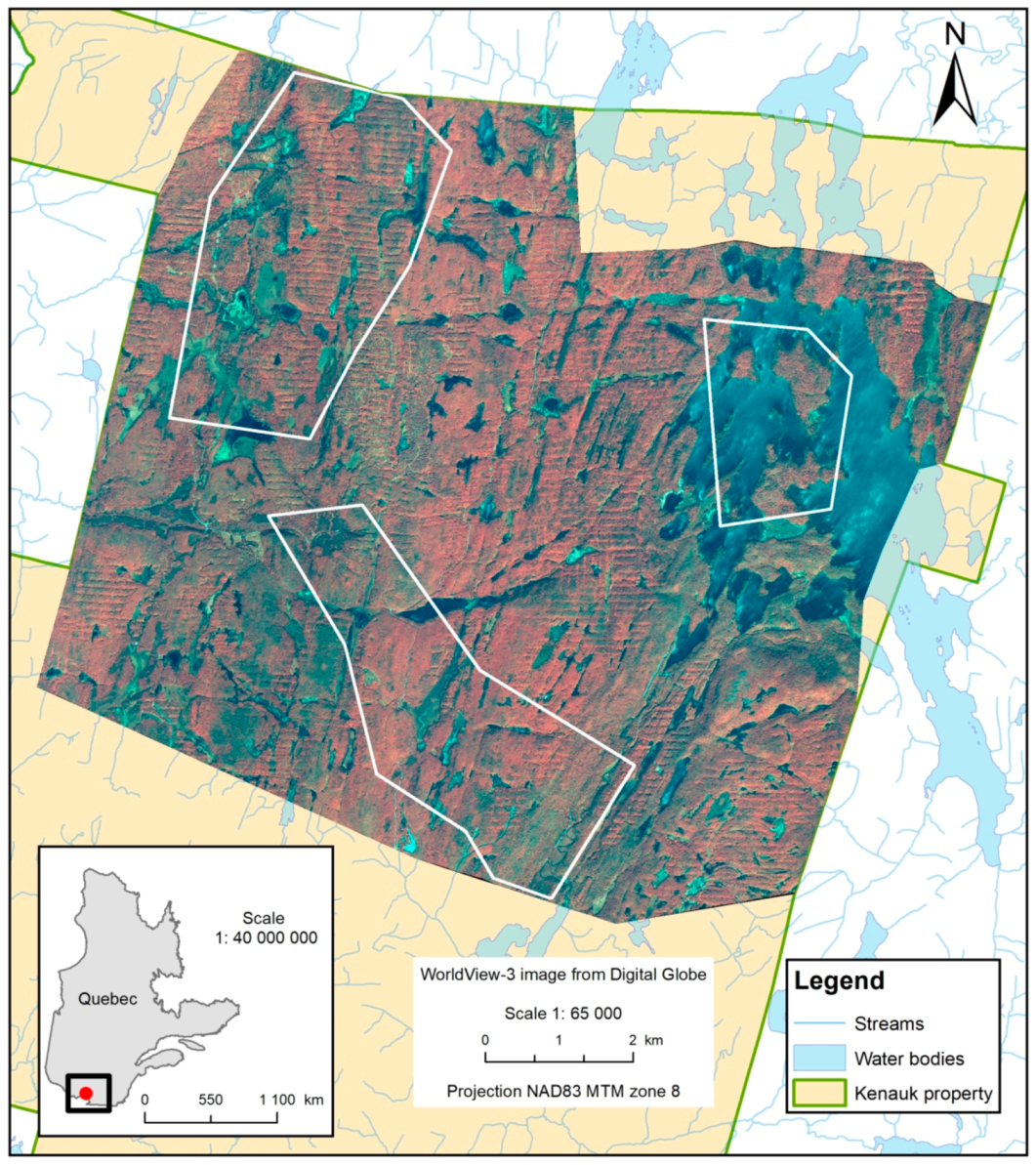
2.1. Study Areas and Data
2.1.1. Study Areas
2.1.2. Imagery and Airborne Laser Scanner Data
2.2. Field Survey and Data Collection
2.3. Derived Variables
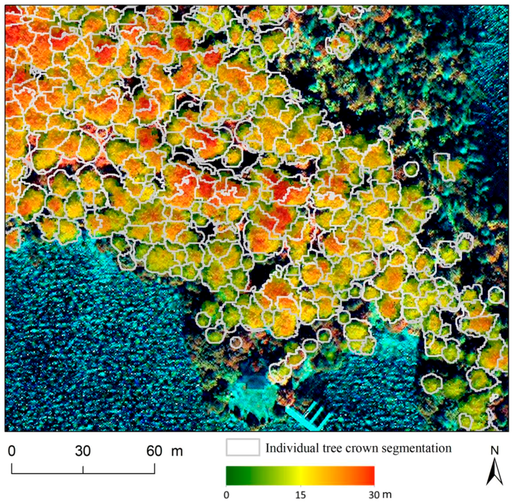
2.4. Tree Crown Segmentation from Fused Data
2.5. Classification Models
2.5.1. Variable Selection
2.5.2. Modeling Process
2.6. Model Performance
3. Results
3.1. Individual Tree Crown Segmentation and Assessment
3.2. Classification and Assessment
4. Discussion
5. Conclusions
Author Contributions
Funding
Acknowledgments
Conflicts of Interest
Appendix A

| Type | Abbreviation | Spectral Variable | Description/Adapted Formula | Reference | Pixel-Based | Higher 95% | Arithmetic Feature | Total Number |
|---|---|---|---|---|---|---|---|---|
| Calculated on band | Band_X_mean | Band 1 to 16 | Arithmetic mean value of band X of the pixels forming the object | x | 16 | |||
| Standard_deviation_Band_X | Band 1 to 16 | Standard deviation of band X of the pixels forming the object | x | 16 | ||||
| Skewness_Band_X | Band 1 to 16 | Skewness of band X of the pixels forming the object | x | 16 | ||||
| Band_X_mean_95pc_highest | Band 1 to 16 | Arithmetic mean of the 5% higher pixel value of the object | x | 16 | ||||
| Spectral indices | ARI | Anthocyanin Reflectance Index | 1/B3 − 1/B6 | [115] | x | x | x | 3 |
| ARI2 | Anthocyanin Reflectance Index | 1/B3 − 1/B5 | [115] | x | x | x | 3 | |
| CI | Carter Index | B7/B5 | [128] | x | x | x | 3 | |
| CRI | Carotenoid Reflectance Index | B7 * (1/B2 − 1/B3) | [140] | x | x | x | 3 | |
| CRI2 | Carotenoid Reflectance Index | 1/B2 − 1/B5 | [140] | x | x | x | 3 | |
| DRI | Datt Reflectance Index | (B7 − B14)/(B7 + B14) | [141] | x | x | x | 3 | |
| DWSI | Disease Water Stress Index | B7/B10 | [130] | x | x | x | 3 | |
| GMI1 | Simple NIR/Red-edge Ratio | B8/B6 | [113] | x | x | x | 3 | |
| GMI2 | Simple NIR/Red-edge Ratio | B7/B6 | [113] | x | x | x | 3 | |
| MSI | Moisture Stress Index | B10/B7 | [142] | x | x | x | 3 | |
| MSISR | Ratio MSI/simple ratio | (B10/B7)/(B8/B5) | [143] | x | x | x | 3 | |
| NDII | Normalized Difference Infrared Index | (B7 − B11)/(B7 + B11) | [144] | x | x | x | 3 | |
| NDLI | Normalized Difference Lignin Index | [log(1/B12) − log(1/B11)]/[log(1/B12) + log(1/B11)] | [145] | x | x | x | 3 | |
| NDNI | Normalized Difference Nitrogen Index | [log(1/B10) − log(1/B11)]/[log(1/B10) + log(1/B11)] | [145] | x | x | x | 3 | |
| NDVI1 | Normalized Difference Vegetation Index | (B7 − B5 )/(B7 + B5) | [128] | x | x | x | 3 | |
| NDVI2 | Normalized Difference Vegetation Index | (B8 − B5 )/(B8 + B5) | [127] | x | x | x | 3 | |
| NDWI | Normalized Difference Water Index | (B7 − B9)/(B7 + B9) | [146] | x | x | x | 3 | |
| NDWI2130 | Normalized Difference Water Index | (B7 − B13)/(B7 + B13) | [147] | x | x | x | 3 | |
| NMDI | Normalized Multi-Band Drought Index | [RB7 − (B11 − B13)]/[B7 + (B11 − B13)] | [148] | x | x | x | 3 | |
| PBI | Plant Biochemical Index | B7/B3 | [129] | x | x | x | 3 | |
| PRI1 | Normalized difference Physiological Reflectance Index | (B2 − B3)/(B2 + B3) | [149,150] | x | x | x | 3 | |
| PRI2 | Normalized difference Physiological Reflectance Index | (B3 − B4)/(B3 + B4) | [149,150] | x | x | x | 3 | |
| PSRI1 | Plant Senescence Reflectance Index | (B5 − B2)/B7 | [150] | x | x | x | 3 | |
| PSRI2 | Plant Senescence Reflectance Index | (B5 − B2)/B6 | [150] | x | x | x | 3 | |
| R5R7 | Ratio of Landsat TM band 5 to band 7 | B11/B14 | [151] | x | x | x | 3 | |
| RENDVI | Red-edge Normalized Difference Vegetation Index | (B7 − B6)/(B7 + B6) | [127] | x | x | x | 3 | |
| RGR1 | Simple Red/Green ratio | B5/B2 | [150] | x | x | x | 3 | |
| SIPI | Structure Insensitive Pigment Index | (B7 − B2)/(B7 + B5) | [116,150] | x | x | x | 3 | |
| Sredgreen | Simple Red/Green ratio | B5/B3 | [117] | x | x | x | 3 | |
| SRWI | Simple Ratio Water Index | B7/B9 | [152] | x | x | x | 3 | |
| TCP_brightness | Tasseled Cap—Brightness | (B2 * 0.3029)+(B3 * 0.2786)+(B5 * 0.4733)+ (B7 * 0.5599)+(B10 * 0.508)+(B14 * 0.1872) | [118] | x | x | x | 3 | |
| TCP_greeness | Tasseled Cap—Green Vegetation Index | (B2 * −0.2941)+(B3 * −0.243)+(B5 * −0.5424)+ (B7 * 0.7276)+(B10 * 0.0713)+(B14 * −0.1608) | [118] | x | x | x | 3 | |
| TCP_wetness | Tasseled Cap—Wetness | (B2 * 0.1511)+(B3 * 0.1973)+(B5 * 0.3283)+ (B7 * 0.3407)+(B10 * −0.7117)+(B14 * −0.4559) | [118] | x | x | x | 3 | |
| VARI | Visible Atmospherically Resistant Index | (B3 − B5)/(B5 + B3 − B2) | [140] | x | x | x | 3 | |
| Vigreen | Visible Atmospherically Resistant Indices Green | (B3 − B5)/(B5 + B3) | [140] | x | x | x | 3 | |
| WBI | Water Band Index | B7/B8 | [153] | x | x | x | 3 | |
| IHS_Hue_Band_5_3_2 | Intensity, hue, saturation (HIS) transformation | Hue calculated with B5, B3 and B2 as red, green and blue | [94] | x | 1 | |||
| IHS_Hue_Band_7_3_2 | Intensity, hue, saturation (HIS) transformation | Hue calculated with B7, B3 and B2 as red, green and blue | [94] | x | 1 | |||
| IHS_Sat_Band_5_3_2 | Intensity, hue, saturation (HIS) transformation | Saturation calculated with B5, B3 and B2 as red, green and blue | [94] | x | 1 | |||
| IHS_Sat_Band_7_3_2 | Intensity, hue, saturation (HIS) transformation | Saturation calculated with B7, B3 and B2 as red, green and blue | [94] | x | 1 | |||
| Textures | GLCM_Contrast_ Band_X | Band 1 to 16 | Contrast calculated with the pixels forming an object | [111] | x | 16 | ||
| GLCM_Dissimilarity_ Band_X | Band 1 to 16 | Dissimilarity calculated with the pixels forming an object | [111] | x | 16 | |||
| GLCM_Entropy_ Band_X | Band 1 to 16 | Entropy calculated with the pixels forming an object | [111] | x | 16 | |||
| GLCM_Homogeneity_ Band_X | Band 1 to 16 | Homogeneity calculated with the pixels forming an object | [111] | x | 16 | |||
| Total | 232 |
References
- Leboeuf, A.; Vaillancourt, É. Guide de Photo-Interprétation des Essences Forestières du Québec Méridional—Édition 2015; Direction des Inventaires Forestiers du MFFP: Québec, QC, Canada, 2015; p. 72. [Google Scholar]
- Berger, J.-P. Norme de Stratification Écoforestière-Quatrième Inventaire Écoforestier; Comité Permanent de la Stratification Forestière de la Direction des Inventaires Forestiers du MRNFQ et Forêt Québec: Québec, QC, Canada, 2008; p. 64. ISBN 978-2-550-73857-2. [Google Scholar]
- Wulder, M.A.; White, J.C.; Hay, G.J.; Castilla, G. Towards automated segmentation of forest inventory polygons on high spatial resolution satellite imagery. For. Chron. 2008, 84, 221–230. [Google Scholar] [CrossRef]
- Varin, M.; Joanisse, G.; Ménard, P.; Perrot, Y.; Lessard, G.; Dupuis, M. Utilisation D’images Hyperspectrales en Vue de Générer une Cartographie des Espèces Forestières de Façon Automatisée; Centre D’enseignement et de Recherche en Foresterie de Sainte-Foy Inc. (CERFO): Québec, QC, Canada, 2016; p. 68. [Google Scholar]
- Cho, M.A.; Malahlela, O.; Ramoelo, A. Assessing the utility WorldView-2 imagery for tree species mapping in South African subtropical humid forest and the conservation implications: Dukuduku forest patch as case study. Int. J. Appl. Earth Obs. Geoinf. 2015, 38, 349–357. [Google Scholar] [CrossRef]
- Waser, L.T.; Küchler, M.; Jütte, K.; Stampfer, T. Evaluating the potential of worldview-2 data to classify tree species and different levels of ash mortality. Remote Sens. 2014, 6, 4515–4545. [Google Scholar] [CrossRef]
- Immitzer, M.; Atzberger, C.; Koukal, T. Tree species classification with Random forest using very high spatial resolution 8-band worldView-2 satellite data. Remote Sens. 2012, 4, 2661–2693. [Google Scholar] [CrossRef]
- Maltamo, M.; Vauhkonen, J.; Næsset, E. Forestry Applications of Airborne Laser Scanning-Concepts and Case Studies; Springer: Dordrecht, The Nederlands, 2014; Volume 32, ISBN 978-94-017-8663-8. [Google Scholar]
- Eid, T.; Gobakken, T.; Næsset, E. Comparing stand inventories for large areas based on photo-interpretation and laser scanning by means of cost-plus-loss analyses. Scand. J. For. Res. 2004, 19, 512–523. [Google Scholar] [CrossRef]
- Tompalski, P.; Coops, N.C.; White, J.C.; Wulder, M.A. Simulating the impacts of error in species and height upon tree volume derived from airborne laser scanning data. For. Ecol. Manag. 2014, 327, 167–177. [Google Scholar] [CrossRef]
- Gougeon, F.A.; Cormier, R.; Labrecque, P.; Cole, B.; Pitt, D.; Leckie, D. Individual Tree Crown (ITC) delineation on Ikonos and QuickBird imagery: The Cockburn Island Study. In Proceedings of the 25th Canadian Symposium on Remote Sensing, Montreal, QC, Canada, 14–16 October 2003; pp. 14–16. [Google Scholar]
- Ahmad Zawawi, A.; Shiba, M.; Jemali, N.J.N. Accuracy of LiDAR-based tree height estimation and crown recognition in a subtropical evergreen broad-leaved forest in Okinawa, Japan. For. Syst. 2015, 24. [Google Scholar] [CrossRef]
- Barnes, C.; Balzter, H.; Barrett, K.; Eddy, J.; Milner, S.; Suárez, J. Individual Tree Crown Delineation from Airborne Laser Scanning for Diseased Larch Forest Stands. Remote Sens. 2017, 9, 231. [Google Scholar] [CrossRef]
- Budei, B.C.; St-Onge, B.; Audet, F.-A.; Hopkinson, C. Identifying the genus or species of individual trees using a three-wavelength airborne lidar system. Remote Sens. Environ. 2018, 204, 632–647. [Google Scholar] [CrossRef]
- Koch, B.; Heyder, U.; Weinacker, H. Detection of Individual Tree Crowns in Airborne Lidar Data. Photogramm. Eng. Remote Sens. 2006, 72, 357–363. [Google Scholar] [CrossRef]
- Jakubowski, M.; Li, W.; Guo, Q.; Kelly, M. Delineating Individual Trees from Lidar Data: A Comparison of Vector- and Raster-based Segmentation Approaches. Remote Sens. 2013, 5, 4163–4186. [Google Scholar] [CrossRef]
- Rana, P.; Prieur, J.-F.; Budei, B.C.; St-Onge, B. Towards a Generalized Method for Tree Species Classification Using Multispectral Airborne Laser Scanning in Ontario, Canada. In Proceedings of the IGARSS 2018-2018 IEEE International Geoscience Remote Sensing Symposium, Valencia, Spain, 22–27 July 2018; pp. 5–8749. [Google Scholar]
- Diedershagen, O.; Koch, B.; Weinacker, H. Automatic segmentation and characterisation of forest stand parameters using airborne lidar data, multispectral and fogis data. Int. Arch. Photogramm. Remote Sens. Spat. Inf. Sci. 2004, 36, 208–212. [Google Scholar]
- Machala, M.; Zejdová, L. Forest Mapping Through Object-based Image Analysis of Multispectral and LiDAR Aerial Data. Eur. J. Remote Sens. 2014, 47, 117–131. [Google Scholar] [CrossRef]
- Hyyppa, J.; Kelle, O.; Lehikoinen, M.; Inkinen, M. A segmentation-based method to retrieve stem volume estimates from 3-D tree height models produced by laser scanners. IEEE Trans. Geosci. Remote Sens. 2001, 39, 969–975. [Google Scholar] [CrossRef]
- Gulbe, L. Identification and delineation of individual tree crowns using Lidar and multispectral data fusion. In Proceedings of the 2015 IEEE International Geoscience and Remote Sensing Symposium (IGARSS), Milano, Italy, 26–31 July 2015; pp. 3294–3297. [Google Scholar]
- Sačkov, I.; Sedliak, M.; Kulla, L.; Bucha, T. Inventory of Close-to-Nature Forests Based on the Combination of Airborne LiDAR Data and Aerial Multispectral Images Using a Single-Tree Approach. Forests 2017, 8, 467. [Google Scholar] [CrossRef]
- Hamraz, H.; Contreras, M.A.; Zhang, J. A robust approach for tree segmentation in deciduous forests using small-footprint airborne LiDAR data. Int. J. Appl. Earth Obs. Geoinf. 2016, 52, 532–541. [Google Scholar] [CrossRef]
- Bunting, P.; Lucas, R. The delineation of tree crowns in Australian mixed species forests using hyperspectral Compact Airborne Spectrographic Imager (CASI) data. Remote Sens. Environ. 2006, 101, 230–248. [Google Scholar] [CrossRef]
- Dalponte, M.; Orka, H.O.; Gobakken, T.; Gianelle, D.; Naesset, E. Tree Species Classification in Boreal Forests With Hyperspectral Data. Geosci. Remote Sens. IEEE Trans. 2013, 51, 2632–2645. [Google Scholar] [CrossRef]
- Ghosh, A.; Fassnacht, F.E.; Joshi, P.K.; Koch, B. A framework for mapping tree species combining hyperspectral and LiDAR data: Role of selected classifiers and sensor across three spatial scales. Int. J. Appl. Earth Obs. Geoinf. 2014, 26, 49–63. [Google Scholar] [CrossRef]
- Jones, T.G.; Coops, N.C.; Sharma, T. Assessing the utility of airborne hyperspectral and LiDAR data for species distribution mapping in the coastal Pacific Northwest, Canada. Remote Sens. Environ. 2010, 114, 2841–2852. [Google Scholar] [CrossRef]
- Matsuki, T.; Yokoya, N.; Iwasaki, A. Hyperspectral Tree Species Classification of Japanese Complex Mixed Forest With the Aid of Lidar Data. IEEE J. Sel. Top. Appl. Earth Obs. Remote Sens. 2015, 8, 2177–2187. [Google Scholar] [CrossRef]
- Verlic, A.; Duric, N.; Kokalj, Z.; Marsetic, A.; Simoncic, P.; Ostir, K. Tree species classification using worldview-2 satellite images and laser scanning data in a natural urban forest. Prethod. Priopćenje Prelim. Commun. Šumarski List 2014, 138, 477–488. [Google Scholar]
- Fassnacht, F.E.; Latifi, H.; Stereńczak, K.; Modzelewska, A.; Lefsky, M.; Waser, L.T.; Straub, C.; Ghosh, A. Review of studies on tree species classification from remotely sensed data. Remote Sens. Environ. 2016, 186, 64–87. [Google Scholar] [CrossRef]
- Hartling, S.; Sagan, V.; Sidike, P.; Maimaitijiang, M.; Carron, J. Urban tree species classification using a worldview-2/3 and liDAR data fusion approach and deep learning. Sensors 2019, 19, 1284. [Google Scholar] [CrossRef] [PubMed]
- Pham, L.T.H.; Brabyn, L.; Ashraf, S. Combining QuickBird, LiDAR, and GIS topography indices to identify a single native tree species in a complex landscape using an object-based classification approach. Int. J. Appl. Earth Obs. Geoinf. 2016, 50, 187–197. [Google Scholar] [CrossRef]
- Varin, M.; Joanisse, G.; Dupuis, M.; Perrot, Y.; Gadbois-Langevin, R.; Brochu, J.; Painchaud, L.; Chalghaf, B. Identification Semi-Automatisée D’essences Forestières à Partir D’images Hyperspectrales, Cas du Témiscamingue; Centre D’enseignement et de Recherche en Foresterie de Sainte-Foy Inc. (CERFO): Québec, QC, Canada, 2019; p. 10. [Google Scholar]
- Varin, M.; Gadbois-Langevin, R.; Joanisse, G.; Chalghaf, B.; Perrot, Y.; Marcotte, J.-M.; Painchaud, L.; Cullen, A. Approche Orientée-Objet pour Cartographier le Frêne et L’épinette en Zone Urbaine; Centre D’enseignement et de Recherche en Foresterie de Sainte-Foy Inc. (CERFO): Québec, QC, Canada, 2018; p. 8. [Google Scholar]
- Dalponte, M.; Bruzzone, L.; Gianelle, D. Tree species classification in the Southern Alps based on the fusion of very high geometrical resolution multispectral/hyperspectral images and LiDAR data. Remote Sens. Environ. 2012, 123, 258–270. [Google Scholar] [CrossRef]
- Arenas-Castro, S.; Fernández-Haeger, J.; Jordano-Barbudo, D. Evaluation and Comparison of QuickBird and ADS40-SH52 Multispectral Imagery for Mapping Iberian Wild Pear Trees (Pyrus bourgaeana, Decne) in a Mediterranean Mixed Forest. Forests 2014, 5, 1304–1330. [Google Scholar] [CrossRef]
- Dube, T.; Mutanga, O.; Elhadi, A.; Ismail, R. Intra-and-Inter Species Biomass Prediction in a Plantation Forest: Testing the Utility of High Spatial Resolution Spaceborne Multispectral RapidEye Sensor and Advanced Machine Learning Algorithms. Sensors 2014, 14, 15348–15370. [Google Scholar] [CrossRef]
- van Ewijk, K.Y.; Randin, C.F.; Treitz, P.M.; Scott, N.A. Predicting fine-scale tree species abundance patterns using biotic variables derived from LiDAR and high spatial resolution imagery. Remote Sens. Environ. 2014, 150, 120–131. [Google Scholar] [CrossRef]
- Alonso-Benito, A.; Arroyo, L.; Arbelo, M.; Hernández-Leal, P. Fusion of WorldView-2 and LiDAR Data to Map Fuel Types in the Canary Islands. Remote Sens. 2016, 8, 669. [Google Scholar] [CrossRef]
- He, Y.; Yang, J.; Caspersen, J.; Jones, T. An Operational Workflow of Deciduous-Dominated Forest Species Classification: Crown Delineation, Gap Elimination, and Object-Based Classification. Remote Sens. 2019, 11, 2078. [Google Scholar] [CrossRef]
- van Deventer, H.; Cho, M.A.; Mutanga, O. Improving the classification of six evergreen subtropical tree species with multi-season data from leaf spectra simulated to WorldView-2 and RapidEye. Int. J. Remote Sens. 2017, 38, 4804–4830. [Google Scholar] [CrossRef]
- Mutlu, M.; Popescu, S.C.; Stripling, C.; Spencer, T. Mapping surface fuel models using lidar and multispectral data fusion for fire behavior. Remote Sens. Environ. 2008, 112, 274–285. [Google Scholar] [CrossRef]
- Ke, Y.; Quackenbush, L.J.; Im, J. Synergistic use of QuickBird multispectral imagery and LIDAR data for object-based forest species classification. Remote Sens. Environ. 2010, 114, 1141–1154. [Google Scholar] [CrossRef]
- Fang, F.; McNeil, B.E.; Warner, T.A.; Maxwell, A.E. Combining high spatial resolution multi-temporal satellite data with leaf-on LiDAR to enhance tree species discrimination at the crown level. Int. J. Remote Sens. 2018, 39, 1–19. [Google Scholar] [CrossRef]
- Li, D.; Ke, Y.; Gong, H.; Li, X. Object-Based Urban Tree Species Classification Using Bi-Temporal WorldView-2 and WorldView-3 Images. Remote Sens. 2015, 7, 16917–16937. [Google Scholar] [CrossRef]
- Kukunda, C.B.; Duque-Lazo, J.; González-Ferreiro, E.; Thaden, H.; Kleinn, C. Ensemble classification of individual Pinus crowns from multispectral satellite imagery and airborne LiDAR. Int. J. Appl. Earth Obs. Geoinf. 2018, 65, 12–23. [Google Scholar] [CrossRef]
- Maxwell, A.E.; Warner, T.A.; Fang, F. Implementation of machine-learning classification in remote sensing: An applied review. Int. J. Remote Sens. 2018, 39, 2784–2817. [Google Scholar] [CrossRef]
- Hawryło, P.; Bednarz, B.; Wężyk, P.; Szostak, M. Estimating defoliation of Scots pine stands using machine learning methods and vegetation indices of Sentinel-2. Eur. J. Remote Sens. 2018, 51, 194–204. [Google Scholar] [CrossRef]
- Nay, J.; Burchfield, E.; Gilligan, J. A machine-learning approach to forecasting remotely sensed vegetation health. Int. J. Remote Sens. 2018, 39, 1800–1816. [Google Scholar] [CrossRef]
- Vaughn, R.N.; Asner, P.G.; Brodrick, G.P.; Martin, E.R.; Heckler, W.J.; Knapp, E.D.; Hughes, F.R. An Approach for High-Resolution Mapping of Hawaiian Metrosideros Forest Mortality Using Laser-Guided Imaging Spectroscopy. Remote Sens. 2018, 10, 502. [Google Scholar] [CrossRef]
- Wu, C.; Chen, W.; Cao, C.; Tian, R.; Liu, D.; Bao, D. Diagnosis of Wetland Ecosystem Health in the Zoige Wetland, Sichuan of China. Wetlands 2018, 38, 469–484. [Google Scholar] [CrossRef]
- Anderson, K.E.; Glenn, N.F.; Spaete, L.P.; Shinneman, D.J.; Pilliod, D.S.; Arkle, R.S.; McIlroy, S.K.; Derryberry, D.R. Estimating vegetation biomass and cover across large plots in shrub and grass dominated drylands using terrestrial lidar and machine learning. Ecol. Indic. 2018, 84, 793–802. [Google Scholar] [CrossRef]
- Matasci, G.; Hermosilla, T.; Wulder, M.A.; White, J.C.; Coops, N.C.; Hobart, G.W.; Zald, H.S.J. Large-area mapping of Canadian boreal forest cover, height, biomass and other structural attributes using Landsat composites and lidar plots. Remote Sens. Environ. 2018, 209, 90–106. [Google Scholar] [CrossRef]
- Zhang, C.; Denka, S.; Cooper, H.; Mishra, D.R. Quantification of sawgrass marsh aboveground biomass in the coastal Everglades using object-based ensemble analysis and Landsat data. Remote Sens. Environ. 2018, 204, 366–379. [Google Scholar] [CrossRef]
- Franklin, S.E.; Skeries, E.M.; Stefanuk, M.A.; Ahmed, O.S. Wetland classification using Radarsat-2 SAR quad-polarization and Landsat-8 OLI spectral response data: A case study in the Hudson Bay Lowlands Ecoregion. Int. J. Remote Sens. 2018, 39, 1615–1627. [Google Scholar] [CrossRef]
- Liu, T.; Abd-Elrahman, A.; Morton, J.; Wilhelm, V.L. Comparing fully convolutional networks, random forest, support vector machine, and patch-based deep convolutional neural networks for object-based wetland mapping using images from small unmanned aircraft system. GISsci. Remote Sens. 2018, 55, 243–264. [Google Scholar] [CrossRef]
- Whyte, A.; Ferentinos, K.P.; Petropoulos, G.P. A new synergistic approach for monitoring wetlands using Sentinels-1 and 2 data with object-based machine learning algorithms. Environ. Model. Softw. 2018, 104, 40–54. [Google Scholar] [CrossRef]
- Ada, M.; San, B.T. Comparison of machine-learning techniques for landslide susceptibility mapping using two-level random sampling (2LRS) in Alakir catchment area, Antalya, Turkey. Nat. Hazards 2018, 90, 237–263. [Google Scholar] [CrossRef]
- Kalantar, B.; Pradhan, B.; Naghibi, S.A.; Motevalli, A.; Mansor, S. Assessment of the effects of training data selection on the landslide susceptibility mapping: A comparison between support vector machine (SVM), logistic regression (LR) and artificial neural networks (ANN). Geomat. Nat. Hazards Risk. 2018, 9, 49–69. [Google Scholar] [CrossRef]
- Wessel, M.; Brandmeier, M.; Tiede, D. Evaluation of different machine learning algorithms for scalable classification of tree types and tree species based on Sentinel-2 data. Remote Sens. 2018, 10, 1419. [Google Scholar] [CrossRef]
- Vapnik, V.N. The Nature of Statistical Learning Theory; Springer: Berlin, Germany, 1995; ISBN 0-387-94559-8. [Google Scholar]
- Bennett, K.P.; Campbell, C. Support Vector Machines: Hype or Hallelujah? SIGKDD Explor. Newsl. 2000, 2, 1–13. [Google Scholar] [CrossRef]
- Huang, C.-L.; Wang, C.-J. A GA-based feature selection and parameters optimizationfor support vector machines. Expert Syst. Appl. 2006, 31, 231–240. [Google Scholar] [CrossRef]
- Scholkopf, B.; Smola, A.J. Learning with Kernels: Support Vector Machines, Regularization, Optimization, and Beyond; MIT Press: Cambridge, MA, USA, 2001; p. 644. ISBN 0262194759. [Google Scholar]
- Pedregosa, F.; Varoquaux, G.; Gramfort, A.; Michel, V.; Thirion, B.; Grisel, O.; Blondel, M.; Prettenhofer, P.; Weiss, R.; Dubourg, V.; et al. Scikit-learn: Machine Learning in Python. J. Mach. Learn. Res. 2011, 12, 2825–2830. [Google Scholar]
- Melgani, F.; Bruzzone, L. Classification of hyperspectral remote sensing images with support vector machines. IEEE Trans. Geosci. Remote Sens. 2004, 42, 1778–1790. [Google Scholar] [CrossRef]
- Camps-Valls, G.; Bruzzone, L. Kernel-based methods for hyperspectral image classification. IEEE Trans. Geosci. Remote Sens. 2005, 43, 1351–1362. [Google Scholar] [CrossRef]
- Lawrence, R.L.; Wright, A. Rule-based classification systems using classification and regression tree (CART) analysis. Photogramm. Eng. Remote. Sens. 2001, 67, 1137–1142. [Google Scholar]
- Breiman, L.; Friedman, J.; Stone, C.J.; Olshen, R.A. Classification and Regression Trees; Taylor & Francis: Abingdon, UK, 1984; p. 368. ISBN 9780412048418. [Google Scholar]
- Breiman, L. Random Forests. Mach. Learn. 2001, 45, 5–32. [Google Scholar] [CrossRef]
- Mao, W.; Wang, F.-Y. (Eds.) Chapter 8-Cultural Modeling for Behavior Analysis and Prediction. In New Advances in Intelligence and Security Informatics; Academic Press: Boston, MA, USA, 2012; pp. 91–102. ISBN 978-0-12-397200-2. [Google Scholar]
- Cutler, D.R.; Edwards, T.C.; Beard, K.H.; Cutler, A.; Hess, K.T.; Gibson, J.; Lawler, J.J. Random forests for classification in ecology. Ecology 2007, 88, 2783–2792. [Google Scholar] [CrossRef]
- Kavzoglu, T. Chapter 33-Object-Oriented Random Forest for High Resolution Land Cover Mapping Using Quickbird-2 Imagery. In Handbook of Neural Computation; Samui, P., Sekhar, S., Balas, V.E., Eds.; Academic Press: Cambridge, MA, USA, 2017; pp. 607–619. ISBN 978-0-12-811318-9. [Google Scholar]
- Altman, N.S. An Introduction to Kernel and Nearest-Neighbor Nonparametric Regression. Am. Stat. 1992, 46, 175–185. [Google Scholar] [CrossRef]
- Meerdink, S.K.; Roberts, D.A.; Roth, K.L.; King, J.Y.; Gader, P.D.; Koltunov, A. Classifying California plant species temporally using airborne hyperspectral imagery. Remote Sens. Environ. 2019, 232, 111308. [Google Scholar] [CrossRef]
- Pu, R.; Landry, S.; Yu, Q. Assessing the potential of multi-seasonal high resolution Pléiades satellite imagery for mapping urban tree species. Int. J. Appl. Earth Obs. Geoinf. 2018, 71, 144–158. [Google Scholar] [CrossRef]
- Ferreira, M.P.; Zortea, M.; Zanotta, D.C.; Shimabukuro, Y.E.; de Souza Filho, C.R. Mapping tree species in tropical seasonal semi-deciduous forests with hyperspectral and multispectral data. Remote Sens. Environ. 2016, 179, 66–78. [Google Scholar] [CrossRef]
- Immitzer, M.; Stepper, C.; Böck, S.; Straub, C.; Atzberger, C. Use of WorldView-2 stereo imagery and National Forest Inventory data for wall-to-wall mapping of growing stock. For. Ecol. Manag. 2016, 359, 232–246. [Google Scholar] [CrossRef]
- Tharwat, A.; Gaber, T.; Ibrahim, A.; Hassanien, A.E. Linear discriminant analysis: A detailed tutorial. AI Commun. 2017, 30, 169–190. [Google Scholar] [CrossRef]
- Hidayat, S.; Matsuoka, M.; Baja, S.; Rampisela, D.A. Object-based image analysis for sago palm classification: The most important features from high-resolution satellite imagery. Remote Sens. 2018, 10, 1319. [Google Scholar] [CrossRef]
- Gosselin, J. Guide de Reconnaissance des Types Écologiques de la Région Écologique 2a–Collines de la Basse-Gatineau; Ministère des Ressources Naturelles, de la Faune et des Parcs, Forêt Québec, Direction des Inventaires Forestiers, Division de la Classification Écologique et Productivité des Stations: Québec, QC, Canada, 2004; p. 184. ISBN 2-551-22454-3. [Google Scholar]
- Lin, C.; Wu, C.-C.; Tsogt, K.; Ouyang, Y.-C.; Chang, C.-I. Effects of atmospheric correction and pansharpening on LULC classification accuracy using WorldView-2 imagery. Inf. Process. Agric. 2015, 2, 25–36. [Google Scholar] [CrossRef]
- Koukoulas, S.; Blackburn, G.A. Mapping individual tree location, height and species in broadleaved deciduous forest using airborne LIDAR and multi-spectral remotely sensed data. Int. J. Remote Sens. 2005, 26, 431–455. [Google Scholar] [CrossRef]
- Zhou, Y.; Qiu, F. Fusion of high spatial resolution WorldView-2 imagery and LiDAR pseudo-waveform for object-based image analysis. ISPRS J. Photogramm. Remote Sens. 2015, 101, 221–232. [Google Scholar] [CrossRef]
- Azevedo, S.C.; Silva, E.A.; Pedrosa, M. Shadow detection improvment using spectral indices and morphological operators in urban areas in high resolution images. Int. Arch. Photogramm. Remote Sens. Spat. Inf. Sci. 2015, XL-7/W3, 587–592. [Google Scholar] [CrossRef]
- Mora, B.; Wulder, M.A.; White, J.C. Identifying leading species using tree crown metrics derived from very high spatial resolution imagery in a boreal forest environment. Can. J. Remote Sens. 2010, 36, 332–344. [Google Scholar] [CrossRef]
- R Development Core Team. R: A Language and Environment for Statistical Computing; R Foundation for Statistical Computing: Vienna, Austria, 2018. [Google Scholar]
- SAS Institute Inc. (Ed.) SAS-STAT User’s Guide: Release 9.4 Edition; SAS Institute Inc.: Cary, NC, USA, 2013; ISBN 1-55544-094-0. [Google Scholar]
- Hill, R.A.; Thomson, A.G. Mapping woodland species composition and structure using airborne spectral and LiDAR data. Int. J. Remote Sens. 2005, 26, 3763–3779. [Google Scholar] [CrossRef]
- Leckie, D.; Gougeon, F.; Hill, D.; Quinn, R.; Armstrong, L.; Shreenan, R. Combined high-density lidar and multispectral imagery for individual tree crown analysis. Can. J. Remote Sens. 2003, 29, 633–649. [Google Scholar] [CrossRef]
- McCombs, J.W.; Roberts, S.D.; Evans, D.L. Influence of Fusing Lidar and Multispectral Imagery on Remotely Sensed Estimates of Stand Density and Mean Tree Height in a Managed Loblolly Pine Plantation. For. Sci. 2003, 49, 457–466. [Google Scholar] [CrossRef]
- Holmgren, J.; Persson, Å.; Söderman, U. Species identification of individual trees by combining high resolution LiDAR data with multi-spectral images. Int. J. Remote Sens. 2008, 29, 1537–1552. [Google Scholar] [CrossRef]
- Weinacker, H.; Koch, B.; Heyder, U.; Weinacker, R. Development of filtering, segmentation and modelling modules for lidar and multispectral data as a fundament of an automatic forest inventory system. Int. Arch. Photogramm. Remote Sens. Spat. Inf. Sci. 2004, 36, 1682–1750. [Google Scholar]
- Trimble Germany GmbH. Trimble Germany GmbH eCognition® Developer 9.3.2 for Windows Operating System: Reference Book; Trimble Germany GmbH: Munich, Germany, 2018; p. 510. [Google Scholar]
- Wang, L.; Sousa, W.P.; Gong, P. Integration of object-based and pixel-based classification for mapping mangroves with IKONOS imagery. Int. J. Remote Sens. 2004, 25, 5655–5668. [Google Scholar] [CrossRef]
- Brillinger, D.R. International Encyclopedia of Political Science; SAGE Publications Inc.: Thousand Oaks, CA, USA, 2011; p. 4032. [Google Scholar]
- Doherty, M.C. Automating the process of choosing among highly correlated covariates for multivariable logistic regression. In Proceedings of the SAS Conference Proceedings: Western Users of SAS Software 2008, Los Angeles, CA, USA, 5–7 November 2008; p. 7. [Google Scholar]
- Kursa, M.B.; Rudnicki, W.R. Feature Selection with the Boruta Package. J. Stat. Softw. 2010, 11. [Google Scholar] [CrossRef]
- Chen, Y.-W.; Lin, C.-J. Combining SVMs with Various Feature Selection Strategies. In Feature Extraction: Foundations and Applications; Guyon, I., Nikravesh, M., Gunn, S., Zadeh, L.A., Eds.; Springer: Berlin, Germany, 2006; pp. 315–324. ISBN 978-3-540-35488-8. [Google Scholar]
- Prasad, A.M.; Iverson, L.R.; Liaw, A. Newer Classification and Regression Tree Techniques: Bagging and Random Forests for Ecological Prediction. Ecosystems 2006, 9, 181–199. [Google Scholar] [CrossRef]
- Liaw, A.; Wiener, M. Classification and Regression by randomForest. R News 2002, 2, 18–22. [Google Scholar]
- Venables, W.N.; Ripley, B.D. Modern Applied Statistics with S; Springer: New York, NY, USA, 2002. [Google Scholar]
- Therneau, T.M.; Atkinson, E.J. An Introduction to Recursive Partitioning Using the RPART Routines; Springer: New York, NY, USA, 2015. [Google Scholar]
- Congalton, R.G. A review of assessing the accuracy of classifications of remotely sensed data. Remote Sens. Environ. 1991, 37, 35–46. [Google Scholar] [CrossRef]
- Monserud, R.A.; Leemans, R. Comparing global vegetation maps with the Kappa statistic. Ecol. Model. 1992, 62, 275–293. [Google Scholar] [CrossRef]
- McHugh, M.L. Interrater reliability: The kappa statistic. Biochem. Med. 2012, 22, 276–282. [Google Scholar] [CrossRef]
- Cohen, J. A Coefficient of Agreement for Nominal Scales. Educ. Psychol. Meas. 1960, 20, 37–46. [Google Scholar] [CrossRef]
- Henrich, V.; Jung, A.; Götze, C.; Sandow, C.; Thürkow, D.; Gläßer, C. Development of an online indices database: Motivation, concept and implementation. In Proceedings of the 6th EARSeL Imaging Spectroscopy SIG Workshop Innovative Tool for Scientific and Commercial Environment Applications, Tel Aviv, Israel, 16–18 March 2009. [Google Scholar]
- Hughes, N.M.; Smith, W.K. Seasonal Photosynthesis and Anthocyanin Production in 10 Broadleaf Evergreen Species. Funct. Plant Biol. 2007, 34, 1072–1079. [Google Scholar] [CrossRef] [PubMed]
- Baatz, M.; Schape, A. Multiresolution segmentation—An optimization approach for high quality multi-scale image segmentation. Angew. Geogr. Inf. 2000, 12, 12–23. [Google Scholar]
- Haralick, R.M. Statistical image texture analysis haralick. In Handbook of Pattern Recognition and Image Processing; Young, T.Y., Ed.; Elsevier Science: New York, NY, USA, 1986; pp. 247–279. [Google Scholar]
- Leboeuf, A.; Vaillancourt, É.; Morissette, A.; Pomerleau, I.; Roy, V.; Leboeuf, A. Photographic Interpretation Guide for Forest Species in Southern Québec; Direction des Inventaires Forestiers: Québec, QC, Canada, 2015; ISBN 97825507278732550727878. [Google Scholar]
- Gitelson, A.A.; Merzlyak, M.N. Remote estimation of chlorophyll content in higher plant leaves. Int. J. Remote Sens. 1997, 18, 2691–2697. [Google Scholar] [CrossRef]
- Minocha, R.; Martinez, G.; Lyons, B.; Long, S. Development of a standardized methodology for quantifying total chlorophyll and carotenoids from foliage of hardwood and conifer tree species. Can. J. For. Res. 2009, 39, 849–861. [Google Scholar] [CrossRef]
- Gitelson, A.A.; Merzlyak, M.N.; Zur, Y.; Stark, R.H.; Gritz, U. Non-Destructive and Remote Sensing Techniques for Estimation of Vegetation Status. In Proceedings of the 3rd European Conference on Precision Agriculture, Montpelier, France, 8–11 July 2001; pp. 205–210, 273. [Google Scholar]
- Peñuelas, J.; Gamon, J.A.; Fredeen, A.L.; Merino, J.; Field, C.B. Reflectance indices associated with physiological changes in nitrogen- and water-limited sunflower leaves. Remote Sens. Environ. 1994, 48, 135–146. [Google Scholar] [CrossRef]
- Gamon, J.A.; Surfus, J.S. Assessing leaf pigment content and activity with a reflectometer. New Phytol. 1999, 143, 105–117. [Google Scholar] [CrossRef]
- Kauth, R.J.; Thomas, G.S. The tasselled cap-A graphic description of the spectral-temporal development of agricultural crops as seen by Landsat. In Proceedings of the Symposium on Machine Processing of Remotely Sensed Data, West Lafayette, IN, USA, 29 June–1 July 1976; Institute of Electrical and Electronics Engineers: Piscataway, NJ, USA, 1976; pp. 4B-41–4B-51. [Google Scholar]
- Pham, A.T.; De Grandpre, L.; Gauthier, S.; Bergeron, Y. Gap dynamics and replacement patterns in gaps of the northeastern boreal forest of Quebec. Can. J. For. Res. 2004, 34, 353–364. [Google Scholar] [CrossRef]
- Coops, N.C.; Wulder, M.A.; Culvenor, D.S.; St-Onge, B. Comparison of forest attributes extracted from fine spatial resolution multispectral and lidar data. Can. J. Remote Sens. 2004, 30, 855–866. [Google Scholar] [CrossRef]
- Heinzel, J.; Koch, B. Investigating multiple data sources for tree species classification in temperate forest and use for single tree delineation. Int. J. Appl. Earth Obs. Geoinf. 2012, 18, 101–110. [Google Scholar] [CrossRef]
- Soille, P. Morphological Image Analysis: Principles and Applications, 2nd ed.; Springer: Berlin, Germany, 2003; ISBN 3540429883. [Google Scholar]
- Lebourgeois, V.; Dupuy, S.; Vintrou, É.; Ameline, M.; Butler, S.; Bégué, A. A combined random forest and OBIA classification scheme for mapping smallholder agriculture at different nomenclature levels using multisource data (simulated Sentinel-2 time series, VHRS and DEM). Remote Sens. 2017, 9, 259. [Google Scholar] [CrossRef]
- Krahwinkler, P.; Rossmann, J. Tree species classification and input data evaluation. Eur. J. Remote Sens. 2013, 46, 535–549. [Google Scholar] [CrossRef]
- Kim, M.; Xu, B.; Madden, M. Object-based Vegetation Type Mapping from an Orthorectified Multispectral IKONOS Image using Ancillary Information. In Proceedings of the GEOBIA 2008—GEOgraphic Object Based Image Analysis for the 21st Century, Calgary, AB, Canada, 6 August 2008; pp. 1682–1777. [Google Scholar]
- Ferreira, M.P.; Zortea, M.; Zanotta, D.C.; Feret, J.B.; Souza Filho, C.R. On the use of shortwave infrared for tree species discrimination in tropical semideciduous forest. Int. Arch. Photogramm. Remote Sens. Spat. Inf. Sci. 2015, XL-3/W3. [Google Scholar] [CrossRef]
- Ferreira, M.P.; Zanotta, D.C.; Zortea, M.; Körting, T.S.; Fonseca, L.M.G.; Shimabukuro, Y.E.; Filho, C.R.S. Automatic tree crown delineation in tropical forest using hyperspectral data. In Proceedings of the 2014 IEEE Geoscience and Remote Sensing Symposium, Quebec City, QC, Canada, 13–18 July 2014; pp. 784–787. [Google Scholar]
- Cho, M.A.; Sobhan, I.; Skidmore, A.K.; Leeuw, J. Discriminating species using hyperspectral indices at leaf and canopy scales. Int. Arch. Photogramm. Remote Sens. Spat. Inf. Sci. 2008, 37, 369–376. [Google Scholar]
- Rama Rao, N.; Garg, P.K.; Ghosh, S.K.; Dadhwal, V.K. Estimation of leaf total chlorophyll and nitrogen concentrations using hyperspectral satellite imagery. J. Agric. Sci. 2008, 146, 65–75. [Google Scholar] [CrossRef]
- Apan, A.; Held, A.; Phinn, S.; Markley, J. Detecting sugarcane ‘orange rust’ disease using EO-1 Hyperion hyperspectral imagery. Int. J. Remote Sens. 2004, 25, 489–498. [Google Scholar] [CrossRef]
- Hovi, A.; Korhonen, L.; Vauhkonen, J.; Korpela, I. LiDAR waveform features for tree species classification and their sensitivity to tree- and acquisition related parameters. Remote Sens. Environ. 2016, 173, 224–237. [Google Scholar] [CrossRef]
- Korpela, I.; Ole Ørka, H.; Maltamo, M.; Tokola, T.; Hyyppä, J. Tree species classification using airborne LiDAR-effects of stand and tree parameters, downsizing of training set, intensity normalization, and sensor type. Silva Fenn. 2010, 44, 319–339. [Google Scholar] [CrossRef]
- Shi, L.; Wan, Y.; Gao, X.; Wang, M. Feature Selection for Object-Based Classification of High-Resolution Remote Sensing Images Based on the Combination of a Genetic Algorithm and Tabu Search. Comput. Intell. Neurosci. 2018. [Google Scholar] [CrossRef] [PubMed]
- Tao, Q.; Wu, G.-W.; Wang, F.-Y.; Wang, J. Posterior Probability SVM for Unbalanced Data. IEEE Trans. Neural Netw. 2005, 16, 1561–1573. [Google Scholar] [CrossRef] [PubMed]
- Farquad, M.A.H.; Bose, I. Preprocessing unbalanced data using support vector machine. Decis. Support Syst. 2012, 53, 226–233. [Google Scholar] [CrossRef]
- Chalghaf, B.; Varin, M.; Joanisse, G. Cartographie Fine des Essences Individuelles par une Approche de Modélisation de type «Random Forest», à partir du lidar et de RapidEye; Rapport 2019-04; Centre D’enseignement et de Recherche en Foresterie de Sainte-Foy Inc. (CERFO): Québec, QC, Canada, 2019; p. 29. [Google Scholar]
- Zhang, Y. Problems in the Fusion of Commercial High-Resolution Satellite Images as Well as LANDSAT 7 Images and Initial Solutions. In Proceedings of the commission IV Symposium on Geospatial Theory, Processing and Applications, Ottawa, ON, Canada, 9–12 July 2002; pp. 587–592. [Google Scholar]
- St-Onge, B.; Grandin, S. Estimating the Height and Basal Area at Individual Tree and Plot Levels in Canadian Subarctic Lichen Woodlands Using Stereo WorldView-3 Images. Remote Sens. 2019, 11, 248. [Google Scholar] [CrossRef]
- Paquette, A.; Joly, S.; Messier, C. Explaining forest productivity using tree functional traits and phylogenetic information: Two sides of the same coin over evolutionary scale? Ecol. Evol. 2015, 5, 1774–1783. [Google Scholar] [CrossRef]
- Gitelson, A.A.; Kaufman, Y.J.; Stark, R.; Rundquist, D. Novel algorithms for remote estimation of vegetation fraction. Remote Sens. Environ. 2002, 80, 76–87. [Google Scholar] [CrossRef]
- Datt, B. A New Reflectance Index for Remote Sensing of Chlorophyll Content in Higher Plants: Tests using Eucalyptus Leaves. J. Plant Physiol. 1999, 154, 30–36. [Google Scholar] [CrossRef]
- Hunt, E.R.; Rock, B.N. Detection of changes in leaf water content using Near- and Middle-Infrared reflectances. Remote Sens. Environ. 1989, 30, 43–54. [Google Scholar] [CrossRef]
- Colombo, R.; Meroni, M.; Marchesi, A.; Busetto, L.; Rossini, M.; Giardino, C.; Panigada, C. Estimation of leaf and canopy water content in poplar plantations by means of hyperspectral indices and inverse modeling. Remote Sens. Environ. 2008, 112, 1820–1834. [Google Scholar] [CrossRef]
- Serrano, L.; Ustin, S.L.; Roberts, D.A.; Gamon, J.A.; Peñuelas, J. Deriving Water Content of Chaparral Vegetation from AVIRIS Data. Remote Sens. Environ. 2000, 74, 570–581. [Google Scholar] [CrossRef]
- Serrano, L.; Peñuelas, J.; Ustin, S.L. Remote sensing of nitrogen and lignin in Mediterranean vegetation from AVIRIS data. Remote Sens. Environ. 2002, 81, 355–364. [Google Scholar] [CrossRef]
- Gao, B. NDWI—A normalized difference water index for remote sensing of vegetation liquid water from space. Remote Sens. Environ. 1996, 58, 257–266. [Google Scholar] [CrossRef]
- Chen, D.; Huang, J.; Jackson, T.J. Vegetation water content estimation for corn and soybeans using spectral indices derived from MODIS near-and short-wave infrared bands. Remote Sens. Environ. 2005, 98, 225–236. [Google Scholar] [CrossRef]
- Wang, L.; Qu, J.J. NMDI: A normalized multi-band drought index for monitoring soil and vegetation moisture with satellite remote sensing. Geophys. Res. Lett. 2007, 34. [Google Scholar] [CrossRef]
- Peñuelas, J.; Filella, I.; Gamon, J.A. Assessment of photosynthetic radiation-use efficiency with spectral reflectance. New Phytol. 1995, 131, 291–296. [Google Scholar] [CrossRef]
- Sims, D.A.; Gamon, J.A. Relationships between leaf pigment content and spectral reflectance across a wide range of species, leaf structures and developmental stages. Remote Sens. Environ. 2002, 81, 337–354. [Google Scholar] [CrossRef]
- Elvidge, C.D.; Lyon, R.J.P. Estimation of the vegetation contribution to the 1•65/2•22 μm ratio in airborne thematic-mapper imagery of the Virginia Range, Nevada. Int. J. Remote Sens. 1985, 6, 75–88. [Google Scholar] [CrossRef]
- Zarco-Tejada, P.J.; Ustin, S.L. Modeling canopy water content for carbon estimates from MODIS data at land EOS validation sites. In Proceedings of the IEEE 2001 International Geoscience and Remote Sensing Symposium, Sydney, Australia, 9–13 July 2001; pp. 342–344. [Google Scholar]
- Penuelas, J.; Pinol, J.; Ogaya, R.; Filella, I. Estimation of plant water concentration by the reflectance Water Index WI (R900/R970). Int. J. Remote Sens. 1997, 18, 2869–2875. [Google Scholar] [CrossRef]


| Band | Spectrum | Wavelength Range (nm) | Wavelength Center (nm) | Spatial Resolution (m) |
|---|---|---|---|---|
| 0 | Panchromatic | 450–800 | 625 | 0.31 |
| 1 | Costal | 400–450 | 425 | 1.26 |
| 2 | Blue | 450–510 | 480 | |
| 3 | Green | 510–580 | 545 | |
| 4 | Yellow | 585–625 | 605 | |
| 5 | Red | 630–690 | 660 | |
| 6 | Red-edge | 705–745 | 725 | |
| 7 | Near-infrared #1 | 770–895 | 832.5 | |
| 8 | Near-infrared #2 | 860–1040 | 950 | |
| 9 | Short-Wave Infrared #1 | 1195–1225 | 1210 | 3.89 |
| 10 | Short-Wave Infrared #2 | 1550–1590 | 1570 | |
| 11 | Short-Wave Infrared #3 | 1640–1680 | 1660 | |
| 12 | Short-Wave Infrared #4 | 1710–1750 | 1730 | |
| 13 | Short-Wave Infrared #5 | 2145–2185 | 2165 | |
| 14 | Short-Wave Infrared #6 | 2185–2225 | 2205 | |
| 15 | Short-Wave Infrared #7 | 2235–2285 | 2260 | |
| 16 | Short-Wave Infrared #8 | 2295–2365 | 2330 |
| Species | Acronym | Type | Tree Crowns Statistics | Train | Test | Total | ||
|---|---|---|---|---|---|---|---|---|
| Mean Size (m2) | Mean Height (m) | SD Height (m) | ||||||
| American Beech | AB | BL | 32 | 21 | 4 | 31 | 10 | 41 |
| Big Tooth Aspen | BT | BL | 42 | 25 | 4 | 13 | 5 | 18 |
| Red Oak | RO | BL | 60 | 24 | 3 | 24 | 10 | 34 |
| Sugar Maple | SM | BL | 85 | 24 | 3 | 37 | 9 | 46 |
| Yellow Birch | YB | BL | 63 | 22 | 4 | 36 | 10 | 46 |
| Balsam Fir | BF | CN | 22 | 16 | 3 | 13 | 3 | 16 |
| Eastern White Cedar | EC | CN | 31 | 21 | 5 | 16 | 5 | 21 |
| Eastern Hemlock | HK | CN | 39 | 23 | 3 | 29 | 9 | 38 |
| Red Pine | RP | CN | 59 | 28 | 3 | 15 | 5 | 20 |
| White Pine | WP | CN | 64 | 26 | 4 | 38 | 10 | 48 |
| White Spruce | WS | CN | 35 | 20 | 5 | 7 | 3 | 10 |
| Total | 259 | 79 | 338 | |||||
| Original | Filtered | Corrected | ||||
|---|---|---|---|---|---|---|
| CHM | CHM+Imagery | CHM | CHM+Imagery | CHM | CHM+Imagery | |
| Single crown | 40% | 56% | 60% | 68% | 63% | 64% |
| Single species | 70% | 74% | 73% | 75% | 73% | 82% |
| Based on 8-Band WorldView-3 | Based on 16-Band WorldView-3 | ||||||||||
|---|---|---|---|---|---|---|---|---|---|---|---|
| Model | Technique | No of Variables | Training | Test | No of Variables | Training | Test | ||||
| OA | KIA | OA | KIA | OA | KIA | OA | KIA | ||||
| Global | RF | 8 | 100% | 1.00 | 71% | 0.67 | 9 | 100% | 1.00 | 75% | 0.72 |
| SVM | 10 | 93% | 0.93 | 70% | 0.66 | 10 | 98% | 0.98 | 71% | 0.68 | |
| k-NN | 9 | 72% | 0.68 | 41% | 0.34 | 10 | 78% | 0.76 | 48% | 0.42 | |
| CART | 8 | 74% | 0.70 | 53% | 0.48 | 10 | 71% | 0.68 | 53% | 0.48 | |
| LDA | 11 | 96% | 0.95 | 66% | 0.61 | 11 | 95% | 0.94 | 61% | 0.56 | |
| Based on 8-Band WorldView-3 | Based on 16-Band WorldView-3 | ||||||||||
|---|---|---|---|---|---|---|---|---|---|---|---|
| Model | Technique | No of Variables | Training | Test | No of Variables | Training | Test | ||||
| OA | KIA | OA | KIA | OA | KIA | OA | KIA | ||||
| Tree type | RF | 4 | 100% | 1.00 | 97% | 0.95 | 4 | 100% | 1.00 | 99% | 0.97 |
| SVM | 10 | 100% | 1.00 | 94% | 0.87 | 6 | 100% | 1.00 | 97% | 0.95 | |
| k-NN | 6 | 100% | 1.00 | 97% | 0.95 | 4 | 100% | 1.00 | 97% | 0.95 | |
| CART | 2 | 97% | 0.93 | 92% | 0.85 | 4 | 98% | 0.96 | 92% | 0.85 | |
| LDA | 3 | 97% | 0.93 | 96% | 0.92 | 4 | 100% | 0.99 | 97% | 0.95 | |
| Based on 8-Band WorldView-3 | Based on 16-Band WorldView-3 | ||||||||||
|---|---|---|---|---|---|---|---|---|---|---|---|
| Model | Technique | No of Variables | Training | Test | No of Variables | Training | Test | ||||
| OA | KIA | OA | KIA | OA | KIA | OA | KIA | ||||
| Broadleaf | RF | 6 | 100% | 1.00 | 70% | 0.63 | 6 | 100% | 1.00 | 68% | 0.60 |
| SVM | 10 | 96% | 0.95 | 59% | 0.49 | 10 | 95% | 0.94 | 68% | 0.60 | |
| k-NN | 7 | 79% | 0.73 | 52% | 0.39 | 6 | 83% | 0.78 | 36% | 0.03 | |
| CART | 6 | 75% | 0.68 | 45% | 0.31 | 6 | 77% | 0.70 | 59% | 0.49 | |
| LDA | 10 | 94% | 0.93 | 64% | 0.53 | 9 | 93% | 0.91 | 61% | 0.51 | |
| Conifer | RF | 7 | 100% | 1.00 | 94% | 0.93 | 7 | 100% | 1.00 | 94% | 0.93 |
| SVM | 10 | 96% | 0.95 | 89% | 0.85 | 9 | 100% | 1.00 | 83% | 0.78 | |
| k-NN | 9 | 89% | 0.86 | 83% | 0.79 | 9 | 88% | 0.84 | 89% | 0.85 | |
| CART | 5 | 79% | 0.73 | 77% | 0.71 | 7 | 81% | 0.75 | 69% | 0.60 | |
| LDA | 8 | 99% | 0.99 | 80% | 0.74 | 9 | 100% | 1.00 | 71% | 0.63 | |
| Abbreviation | Vegetation Index | Adapted Formula | Models | References |
|---|---|---|---|---|
| ARI_mean | Anthocyanin Reflectance Index | 1/B3_mean − 1/B6_mean | Conifer | [115] |
| ARI_mean_95pc_higher | Anthocyanin Reflectance Index | Arithmetic mean of the 5% higher pixel value of the object with ARI | Tree type | [115] |
| Band_1_mean | Layer values | Mean value of band 1 of the pixels forming the object | Broadleaf | [6] |
| Band_12_95pc_higher | Layer values | Arithmetic mean of the 5% higher pixel value of the object using band 12 | Tree type | [6] |
| Band_5_95pc_higher | Layer values | Arithmetic mean of the 5% higher pixel value of the object using band 5 | Broadleaf | [6] |
| GLCM_Entropy_Band_7 | Texture values | Entropy calculated with the value of band 7 of the pixels forming an object | Broadleaf; Conifer | [110,111] |
| GLCM_Homogeneity_Band_3 | Texture values | Homogeneity calculated with the value of band 3 of the pixels forming an object | Conifer | [110,111] |
| GLCM_Homogeneity_Band_4 | Texture values | Homogeneity calculated with the value of band 4 of the pixels forming an object | Conifer | [110,111] |
| GMI2_mean | Simple NIR/Red-edge Ratio | B7_mean/B6_mean | Conifer | [113] |
| IHS_Hue_Band_7_3_2 | Intensity, hue, saturation (HIS) transformation | Hue calculated with B7, B3 and B2 as red, green and blue | Conifer | [94,110] |
| PRI2_mean | Normalized difference Physiological Reflectance Index | (B3_mean − B4_mean)/(B3_mean + B4_mean) | Broadleaf | [116] |
| PRI2_mean_95pc_higher | Normalized difference Physiological Reflectance Index | Arithmetic mean of the 5% higher pixel value of the object with PRI2 | Broadleaf | [116] |
| Sredgreen_mean | Simple Red/Green ratio | B5_mean/B3_mean | Conifer | [117] |
| Sredgreen_mean_95pc_higher | Simple Red/Green ratio | Arithmetic mean of the 5% higher pixel value of the object with Sredgreen | Tree type | [117] |
| Standard_deviation_Band_3 | Layer values | Standard deviation of band 3 of the pixels forming the object | Broadleaf | [6] |
| TCP_greeness_mean | Tasselled Cap—Green Vegetation Index | (B2_mean * −0.2941)+(B3_mean * −0.243)+(B5_mean * −0.5424)+(B7_mean * 0.7276)+(B10_mean * 0.0713)+(B14_mean * −0.1608) | Tree type | [118] |
| Band | B1 | B2 | B3 | B4 | B5 | B6 | B7 | B12 | B14 |
|---|---|---|---|---|---|---|---|---|---|
| Times used | 1 | 2 | 10 | 3 | 4 | 3 | 5 | 1 | 1 |
| Reference | |||||||||||||
|---|---|---|---|---|---|---|---|---|---|---|---|---|---|
| AB | BT | RO | SM | YB | BF | EC | HK | RP | WP | WS | User’s Accuracy (%) | ||
| Prediction | AB | 7 | 0 | 0 | 0 | 2 | 0 | 0 | 0 | 0 | 0 | 0 | 78% |
| BT | 0 | 4 | 0 | 0 | 0 | 0 | 0 | 0 | 0 | 0 | 0 | 100% | |
| RO | 0 | 0 | 5 | 1 | 0 | 0 | 0 | 0 | 0 | 0 | 0 | 83% | |
| SM | 1 | 0 | 3 | 7 | 1 | 0 | 0 | 0 | 0 | 0 | 0 | 58% | |
| YB | 1 | 0 | 2 | 1 | 7 | 0 | 0 | 0 | 0 | 0 | 0 | 64% | |
| BF | 0 | 0 | 0 | 0 | 0 | 2 | 0 | 0 | 0 | 0 | 1 | 67% | |
| EC | 1 | 1 | 0 | 0 | 0 | 0 | 4 | 0 | 0 | 0 | 0 | 67% | |
| HK | 0 | 0 | 0 | 0 | 0 | 0 | 0 | 9 | 0 | 0 | 0 | 100% | |
| RP | 0 | 0 | 0 | 0 | 0 | 0 | 1 | 0 | 3 | 0 | 1 | 60% | |
| WP | 0 | 0 | 0 | 0 | 0 | 1 | 0 | 0 | 2 | 10 | 0 | 77% | |
| WS | 0 | 0 | 0 | 0 | 0 | 0 | 0 | 0 | 0 | 0 | 1 | 100% | |
| Producer’s accuracy (%) | 70% | 80% | 50% | 78% | 70% | 67% | 80% | 100% | 60% | 100% | 33% | OA: 75% KIA: 0.72 | |
| Reference | ||||
|---|---|---|---|---|
| Broadleaf | Conifer | User’s Accuracy (%) | ||
| Prediction | Broadleaf | 44 | 1 | 98 |
| Conifer | 0 | 34 | 100 | |
| Producer’s accuracy (%) | 100 | 97 | OA: 99% KIA: 0.97 | |
| Reference | |||||||
|---|---|---|---|---|---|---|---|
| AB | BT | RO | SM | YB | User’s Accuracy (%) | ||
| Prediction | AB | 6 | 0 | 1 | 0 | 1 | 75% |
| BT | 1 | 5 | 0 | 0 | 1 | 71% | |
| RO | 0 | 0 | 6 | 3 | 0 | 67% | |
| SM | 1 | 0 | 1 | 6 | 0 | 75% | |
| YB | 2 | 0 | 2 | 0 | 8 | 67% | |
| Producer’s accuracy (%) | 70% | 60% | 100% | 60% | 67% | OA: 70% KIA: 0.63 | |
| Reference | ||||||||
|---|---|---|---|---|---|---|---|---|
| BF | EC | HK | RP | WP | WS | User’s Accuracy (%) | ||
| Prediction | BF | 3 | 0 | 0 | 0 | 0 | 0 | 100% |
| EC | 0 | 4 | 0 | 0 | 0 | 0 | 100% | |
| HK | 0 | 0 | 9 | 0 | 0 | 0 | 100% | |
| RP | 0 | 0 | 0 | 4 | 0 | 0 | 100% | |
| WP | 0 | 1 | 0 | 1 | 10 | 0 | 83% | |
| WS | 0 | 0 | 0 | 0 | 0 | 3 | 100% | |
| Producer’s accuracy (%) | 100% | 80% | 100% | 80% | 100% | 100% | OA: 94% KIA: 0.93 | |
© 2020 by the authors. Licensee MDPI, Basel, Switzerland. This article is an open access article distributed under the terms and conditions of the Creative Commons Attribution (CC BY) license (http://creativecommons.org/licenses/by/4.0/).
Share and Cite
Varin, M.; Chalghaf, B.; Joanisse, G. Object-Based Approach Using Very High Spatial Resolution 16-Band WorldView-3 and LiDAR Data for Tree Species Classification in a Broadleaf Forest in Quebec, Canada. Remote Sens. 2020, 12, 3092. https://doi.org/10.3390/rs12183092
Varin M, Chalghaf B, Joanisse G. Object-Based Approach Using Very High Spatial Resolution 16-Band WorldView-3 and LiDAR Data for Tree Species Classification in a Broadleaf Forest in Quebec, Canada. Remote Sensing. 2020; 12(18):3092. https://doi.org/10.3390/rs12183092
Chicago/Turabian StyleVarin, Mathieu, Bilel Chalghaf, and Gilles Joanisse. 2020. "Object-Based Approach Using Very High Spatial Resolution 16-Band WorldView-3 and LiDAR Data for Tree Species Classification in a Broadleaf Forest in Quebec, Canada" Remote Sensing 12, no. 18: 3092. https://doi.org/10.3390/rs12183092
APA StyleVarin, M., Chalghaf, B., & Joanisse, G. (2020). Object-Based Approach Using Very High Spatial Resolution 16-Band WorldView-3 and LiDAR Data for Tree Species Classification in a Broadleaf Forest in Quebec, Canada. Remote Sensing, 12(18), 3092. https://doi.org/10.3390/rs12183092