Comparison of Field and Laboratory Wet Soil Spectra in the Vis-NIR Range for Soil Organic Carbon Prediction in the Absence of Laboratory Dry Measurements

Abstract

Spectroscopy has demonstrated the ability to predict specific soil properties. Consequently, it is a promising avenue to complement the traditional methods that are costly and time-consuming. In the visible-near infrared (Vis-NIR) region, spectroscopy has been widely used for the rapid determination of organic components, especially soil organic carbon (SOC) using laboratory dry (lab-dry) measurement. However, steps such as collecting, grinding, sieving and soil drying at ambient (room) temperature and humidity for several days, which is a vital process, make the lab-dry preparation a bit slow compared to the field or laboratory wet (lab-wet) measurement. The use of soil spectra measured directly in the field or on a wet sample remains challenging due to uncontrolled soil moisture variations and other environmental conditions. However, for direct and timely prediction and mapping of soil properties, especially SOC, the field or lab-wet measurement could be an option in place of the lab-dry measurement. This study focuses on comparison of field and naturally acquired laboratory measurement of wet samples in Visible (VIS), Near-Infrared (NIR) and Vis-NIR range using several pretreatment approaches including orthogonal signal correction (OSC). The comparison was concluded with the development of validation models for SOC prediction based on partial least squares regression (PLSR) and support vector machine (SVMR). Nonetheless, for the OSC implementation, we use principal component regression (PCR) together with PLSR as SVMR is not appropriate under OSC. For SOC prediction, the field measurement was better in the VIS range with R²_CV = 0.47 and RMSEPcv = 0.24, while in Vis-NIR range the lab-wet measurement was better with R²_CV = 0.44 and RMSEPcv = 0.25, both using the SVMR algorithm. However, the prediction accuracy improves with the introduction of OSC on both samples. The highest prediction was obtained with the lab-wet dataset (using PLSR) in the NIR and Vis-NIR range with R²_CV = 0.54/0.55 and RMSEPcv = 0.24. This result indicates that the field and, in particular, lab-wet measurements, which are not commonly used, can also be useful for SOC prediction, just as the lab-dry method, with some adjustments.

1. Introduction

Soils are significant natural resources for the survival of humanity. Substantially more carbon is stockpiled in the world’s soils than is present in global vegetation and atmosphere combined [1]. Studies have shown over the years that the conservation of soil organic carbon (SOC) concentrations is strongly linked to biological activity and agricultural productivity [2]. Maintaining SOC contents above critical limits for specific ecological and climatic zones will help to protect soil resources and maintain crop yields, thus contributing to global food security [3]. Prediction of SOC in the soil is, therefore, essential because there is always an improvement in soil health as well as the alleviation of climate change whenever SOC content increases [4].

Soil spectroscopy under proximal soil sensing, developed some decades ago, has been used as a useful tool by more researchers in recent years to complement traditional soil analysis [5,6]. Spectroscopy, being the analysis of the interaction of visible-infrared wavelengths with soil properties, also provides information on soil particle size and thus information on the soil matrix. Another attractive feature of spectroscopy is that spectra can be recorded, at points or by imaging, from different platforms; by proximal sensing in the field, in the laboratory using sampled material, or from remote sensing platforms with multi- and hyperspectral capabilities. Compared with analytical laboratory approaches, its measurement is more cost-effective because it is quicker and can use a single spectral measurement to infer multiple soil properties [5,6,7]. In laboratory and field environments, the spectroscopy technique is increasingly used to predict numerous soil constituents based on their diagnostic spectral features and approaches to statistical regression [8].

Prediction of soil organic carbon using visible near-infrared (Vis-NIR) spectroscopy under laboratory-controlled conditions has produced the most accurate results (high analytical precision) in comparison to field and remote sensing platforms [9,10,11]. Under laboratory conditions, external factors such as moisture and environmental conditions that could influence the spectrum are manipulated and are subject to greater control, e.g., spectral noise and atmospheric attenuation. However, steps such as collection, grinding, sieving, and drying of soil, which are vital during this process, make it slower in comparison to field measurements [12,13].

The laboratory domain has become well acknowledged ahead of using the field and other applications. However, direct and timely prediction and mapping of soil properties, especially SOC, can preferably be accomplished by field spectroscopy measurement [14]. Some researchers have even shown the field measurement producing better results than under the laboratory-controlled approach. For example, working with an exceedingly disturbed savannah-like environment, Nocita et al. [15] detected good field predictions of SOC comparative to the same soil samples verified under laboratory conditions. Also, Stevens et al. [16] demonstrated that field measurements could be as accurate as laboratory measurements by comparing the efficiency of the laboratory, field, and airborne spectroscopy to predict SOC using PLSR. They concluded that the RMSE of the field spectral prediction was similar to that of the Walkley and Black method, and that airborne spectroscopy was inaccurate.

Similarly, understanding the impact of different soil components under field conditions is not extensively known. Nevertheless, for the assessment of the applicability of laboratory studies to the natural system, field conditions remain a fundamental requirement [17]. However, natural variability issues must be taken into consideration when sampling materials in the field, as the field environment can display subtle and complex variability. Soil samples obtained from the field can also undergo chemical reactions if special safeguard measures are not applied. For example, an increase in soil pH as a result of CO₂ degassing is because the atmospheric condition and that of the soil atmosphere differ. These changes in atmospheric condition also affect redox-sensitive elements such as Fe, Cr, Hg, Cu, etc., upon their exposure, especially within a depleted oxygen environment [17].

Another form of dataset using the spectroscopy approach (aside field and laboratory dry data) is laboratory wet data. Ideally, for this form of dataset, the sample is collected from the field and then the spectral measurement is taken immediately upon reaching the laboratory. For the wet sample to remain in its natural state, proper and orderly transportation from the field to the laboratory must be ensured. The laboratory wet spectral measurements have also received some considerable attention over the years by researchers, but rather in an artificial form, through a process called rewetting [18,19,20]. However, in its natural acquired state, it has received relatively less attention. According to Barnard et al. [21] and Bailey et al. [22], when rewetting dry soil, a large pulse of CO₂ is emanated from the soil instantly, known as the ‘Birch Effect’, named after “H.F. Birch” who experienced a high mineralization effect in East African soils after the rewetting process [23]. According to Bailey et al. [22], these outcomes can cause a considerable decline in soil carbon stabilization and may even affect its predictability outcome. According to Sparks [17], introducing water to the soil can also create a solution–solid or solution–gas reaction that may result in an unstable solution–soil equilibrium if the reaction time is either too short or too long. This shows that the addition of water to dry soil under laboratory conditions may put the soil under undesirable conditions even before prediction. Artificially generated wet samples (mostly used for experiments) may differ somewhat from the natural collected wet samples due to the rewetting approach.

The first stage of Vis-NIR spectra-based multivariate calibration is often data preprocessing. The intention for this is that Vis-NIR spectra often constitute a subset of the features including noise, scattering of light and variances in spectroscopic path length, which are unrelated to the responses. The variation in the predictor that is unrelated to response can disrupt the multivariate modeling, leading to an inaccurate prediction. Some of these pretreatment methods end up removing relevant information from the predictor, especially multiple signal correction (MSC) and standard normal variate (SNV) [24]. This could either cause an enhancement or have a weakening effect [25]. Orthogonal signal correction (OSC) was firstly introduced by Wold et al. [24] for NIR spectra correction and later on as an improvement to its performance; numerous algorithms have since been published. The key concept of OSC technique is based on eliminating the variation that is not related to the parameter for estimation. This method is achieved through the removal of nonrelevant information of the response in the matrix. Therefore, only information orthogonal to the response is omitted. This is made by ensuring that the removed portion is mathematically orthogonal to the response, or as near as possible to being orthogonal. In some cases, the OSC method can also remove nonlinear relationships between the response and the predicted variables [24]. Though the method often converges fast, it still needs 5–10 repetitions [26].

The aim of this work is to compare field and naturally acquired lab-wet spectral datasets, in their raw and pretreatment state, and also to verify the impact on the prediction accuracy by the introduction of OSC. We will determine which of these datasets could be more suitable in the absence of a lab-dry measurement or when a quicker analysis is required. This will be accomplished by the use of Vis-NIR spectra and their ranges.

2. Materials and Methods

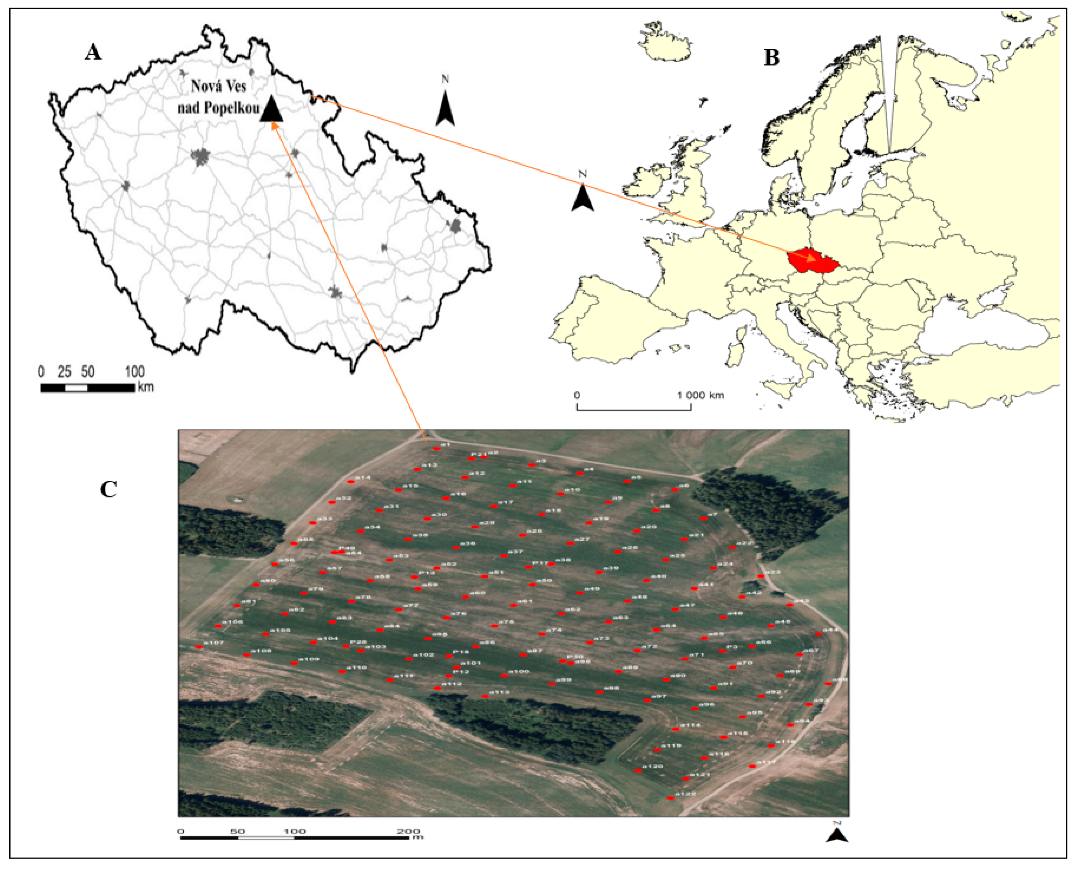
2.1. Study Area

Field spectral data (FSD) were measured in May 2019 on a (not recently ploughed) 22 ha agricultural field located at Nová Ves nad Popelkou (50°31′ N; 15°24′ E), central Bohemian region, with a mean altitude of 185 m a.s.l (Figure 1). The areas are primarily rural and devoted to winter and spring cereals and characterized by dissected relief with side valleys and toe-slopes. The total number of measurement and sampling points over the field was 130. The area chosen was representative of the soils capes that were homogenous and comparable in terms of terrain characteristics, land management, and the climatic conditions [27]. According to the World Reference Base (WRB) for soil resources (IUSS Working Group WRB, 2014), soils of this regions are characterized mainly as Cambisols on sedimentary rocks.

2.2. Soil Sampling and Spectral Measurement

The field spectral measurement was taken instantly in the field using an ASD Field Spec III Pro FR spectroradiometer (ASD Inc., Denver, CO, USA) across the 350–2500 nm wavelength range. The spectroradiometer spectral resolution was 2 nm for the region of 350–1050 nm and 10 nm for the region of 1050–2500 nm. Measurements from four different positions around each of the 130 sampling points were taken, and the average value was used for further analysis. The measurement and sampling points (130) were created before the field visit (Figure 1) and were located in the field using a GeoXM (Trimble Inc., Sunnyvale, CA, USA) receiver with an accuracy of 1 m. The spectrometer was standardized using the approach of Shi et al. [28]. Samples for laboratory analysis were collected from each of those positions (depth 0–20cm) while the field measurement was underway. Composite samples (approximately 150 to 200 g of soil) were placed into a well-labeled bag and transported to the laboratory for further analysis. Immediately upon reaching the laboratory, spectra readings were taken using the same spectrometer used for the field measurement again in four replicates and the average value used as the lab-wet dataset. The samples were then air-dried, gently crushed, and sieved (≤2 mm) before analyzing for SOC (ISO 11464:2006).

2.3. Spectra Pretreatment and Prediction Model Development

Before modeling, lab-wet and field data were preprocessed. The original spectral range is 350–2500 nm; however, the noisy portions between 350–399 nm were eliminated, leaving the range of 400–2500 nm before spectra pretreatments. Murray [29] stated that removing outliers improves prediction accuracy. Therefore, the outliers from both datasets were removed using a local outlier factor (LOF) algorithm procedure proposed by Breunig et al. [30]. The LOF is a measure that looks at a certain point’s neighbours to figure out its density and then compares it with the density of other points and uses its local approach to better detect outliers within the neighborhoods. The field data set was used as the reference data for the removal of outliers, meaning that the removed outliers from the field dataset were the same outliers as removed from the lab-wet dataset. In all, a total of seven outliers were removed from each dataset. With the exception of the orthogonal signal correction (OSC) (using the Unscramble Software, Version X11, CAMO, Oslo, Norway), all other pretreatment methods used were calculated with R software (R Development Core Team, Vienna, Austria, 2015). This pretreatment includes Savitzky-Golay (SG) filtering, discrete wavelet transformation (DWT), multiplicative scatter correction (MSC), standard normal variate (SNV), correction by the maximum reflectance (CMR), continuum removal (CR), first and second-order derivative (D1 and D2 respectively), as well as logarithmic transformation (Log(1/R)). We used the sgolayfilt algorithm from the signal R package for the SG filtering (adjusted for second-order polynomial fit with 30 smoothing points). For more detail about the pretreatment, the packages used can be found in [31,32,33,34].

The PLSR and SVMR predictive models built using five fold leave-group-out cross validation (which was repeated 100× to give more reliable results) were fitted separately, using either raw unsmoothed or smoothed spectra. The models were then adjusted using nine other signal transforms (SG, D1, D2, SNV, log(1/R), DWT, MSC, CR and CMR) with the exception of OSC. All transformations (except SG) were applied in two ways, i.e., the input data were either raw reflectance spectra or smoothed SG spectra and DWT. This was done in the visible (VIS; 400–800), near-infrared (NIR; 800–2500), and the whole Vis-NIR (400–2500) spectral region. In all, there were 24 different output models to be tested for each of the two datasets. Due to insignificant changes and identical performance, only transforms computed from raw spectra are shown, since they were better than using SG in more instances. Almost all the signal transformations were plotted in Figure 2 to visualize differences between different preprocessing methods. However, the reflectance and absorbance plot were separated for visual assessment of variation in the spectra and also their similarities (Figure 3). For the OSC, which is sensitive to the nonlinear algorithm, its assessment was done using PLSR and principal component regression (PCR), not SVMR because SVMR is a nonlinear algorithm. OSC was also done in three spectral regions, just as the nine other signal transformations.

For a detailed comparison of obtained spectra (lab-wet and field), that is, to determine the stable part of the spectra (the part not affected by moisture), the part that differs, and the part with no meaningful information, many options were explored without any significant success. Finally, we used three different combinations to analyze the datasets: median filter smoothing (MFS) with segment size of 7, spectroscopic transformation-absorbance (STA) and gap-segment second derivative (GSD) having a gap size of 6, and a segment size of 25 (Unscramble Software, Version X11, CAMO, Oslo, Norway). The order was MFS–STA–GSD.

3. Results

3.1. SOC Descriptive Statistics

Table 1. Descriptive statistics of the soil’s soil organic carbon (SOC) contents in the study area.

Property	Mean	Median	SD	SV	Kurtosis	Skewness	Range	Min	Max	CV(%)
SOC content (%) (n = 130)	1.44	1.44	0.33	0.11	2.41	0.57	2.33	0.60	2.93	23.00
SD: standard deviation, CV: coefficient of variation, n: number of samples, SV: sample variance

is a summary statistic for SOC characteristic of soil sample in the study area, consisting of standard deviation (SD), coefficient of variation (CV), minimum, maximum, mean value, skewness and range. The statistical distributions of SOC at the study area were positively skewed with a mean value of 1.44 and a CV of 23%. These values usually indicate that the area has a medium to semi-high SOC content.

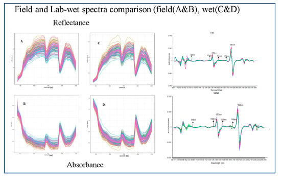
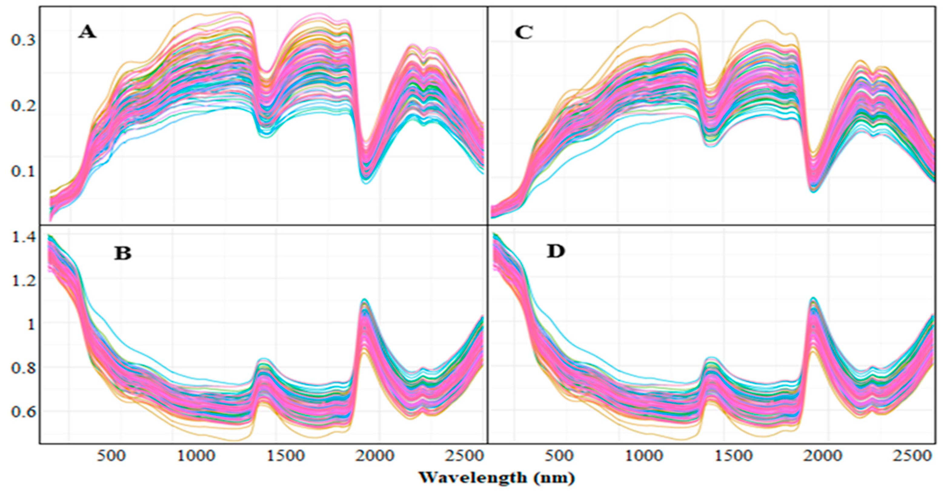
3.2. Basic Comparison of Field And Lab-Wet Spectra

Figure 3 shows the reflectance and absorbance plot from the raw data for each dataset, which was done to explore the patterns and structure of the generated spectra. The key spectral characteristics of a range of soil samples can be perceived from its mean score spectrum, which indicates the average reflectance as well as absorbance in each spectral band for the entire sample sets and the band-specific spectral variance crosswise the total spectral region.

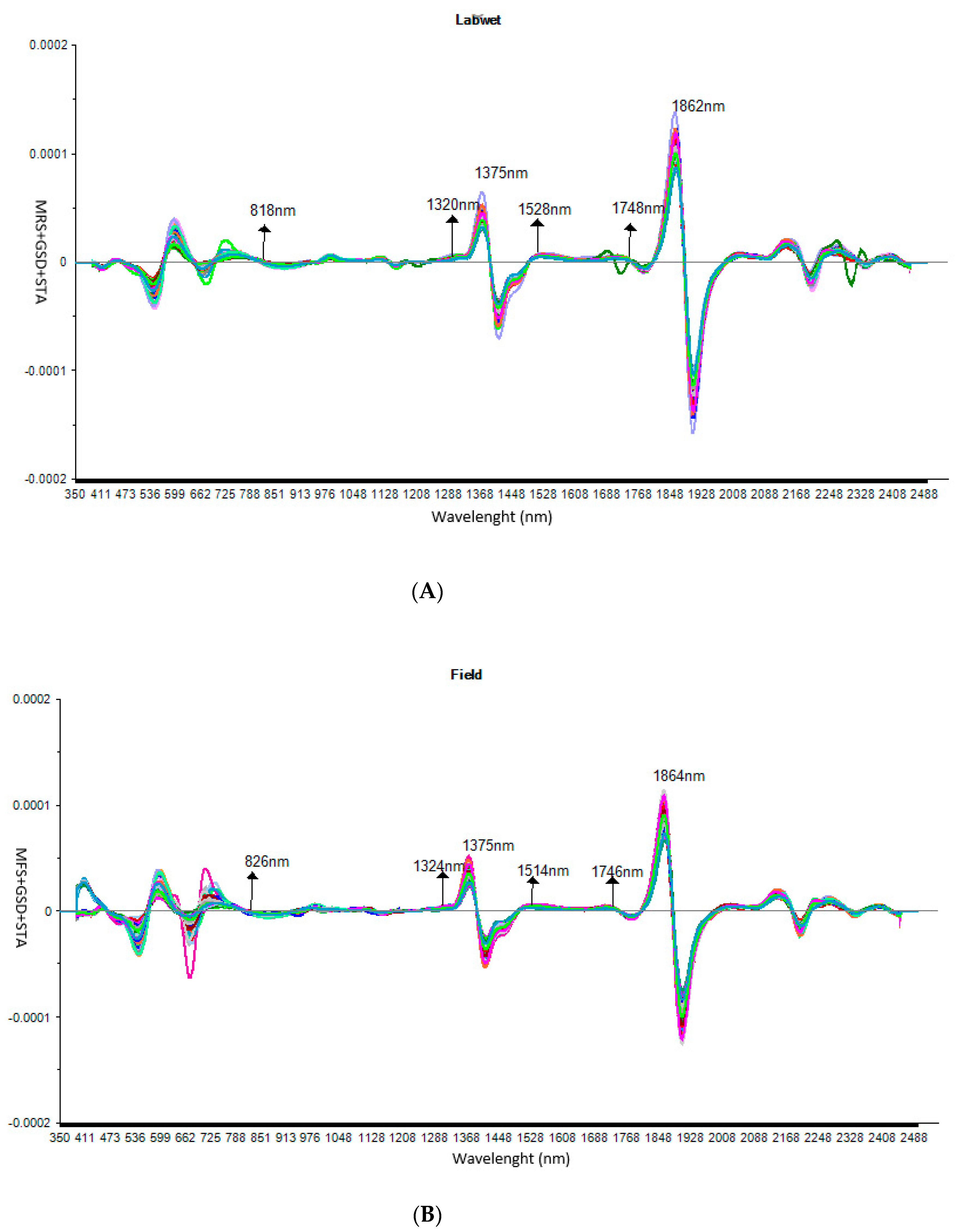
3.3. Detailed Comparison of Field and Lab-Wet Transformed Spectra

As shown by this work (Figure 4), the stable range for lab-wet spectra is from 818 nm to 1320 nm and from 1528 to 1748 nm. For field, it is located between 826 nm and 1324 nm and between 1514 and 1746 nm. This section is categorized as a region that is not influenced by moisture. The concave shape between 450 and 850 nm suggests the presence of crystalline iron [35]. This is also in agreement with Dematte et al. [36] as they stated that soil minerals containing iron, such as hematite and goethite, result in concave shapes in the visible region of the spectrum. Nevertheless, spectra regions below 820 nm do not show any significant information for either dataset due to noise. However, this is not a justification that this range will not be suitable for prediction, but rather should be interpreted on a case-by-case basis. For example, Islam et al. [37] and Fystro [38] achieved a significantly better result for both Australian and Norwegian soils by using the visible region (350–700 nm) for prediction of SOC. This study also shows that both lab-wet and field spectra between the range of 2000 and 2400 nm display more irregular and unstable patterns, which could be attributed to the relatively low level of incoming radiation for the acquired spectra in the field resulting from the high noise rate. For the lab-wet spectra, this could just be noise or maybe other factors which, for this work, will be very difficult to explain. Poor absorption at 2265 nm for both lab-wet and field suggests the presence of gibbsite [39]. According to research by Howari et al. [40], the absorption characteristics at 990 nm are due to the presence of NaCl, while NaHCO₃ shows the absorption characteristics at 1470 nm, 1990 nm and 2170 nm. Absorption at 1400 nm is typically due to vibrations of water molecules and OH groups.

The spectrum shown in Figure 4 also illustrates one significant disparity between the field and lab-wet datasets. While the lab-wet dataset displays its peak absorbance value at 1862 nm, the field dataset shows its peak at a shifted wavelength of 1864 nm. Peak shifts are expected due to the effect of temperature change that a sample can sometimes undergo. This could say something about both the physics and chemistry of the determined samples. It may be a risky attempt to remove/mask it because one does not know whether the procedure will end up with the removal of a real and existing signal. Another peak between 1320 and 1528 nm is at the same wavelength of 1375 nm in both field and lab-wet datasets.

However, a concern about the application of field and lab-wet spectra remains because their reflectance may be heavily influenced by moisture content, though Vis-NIR spectroscopy can effectively measure samples with moisture content. Therefore, using any of them as a replacement to the dry spectra may be seen as a wrong decision, because predictive ability and accuracy of Vis-NIR measurement is negatively affected by moisture [41,42,43]. Despite this, some studies have shown that the field spectra can be more effective than lab-dry measurement for SOC prediction, and Reeves et al. [44] even stated that in the absence of lab-dry measurement, the field spectra should be considered as the most appropriate spectral measurement.

3.4. Comparing Field and Lab-Wet Spectra Predictive Capabilities without OSC

PLSR and SVMR, together with several pretreatment methods, were initially used to compare the prediction accuracy for both field and lab-wet spectral datasets. Leave-group-out cross validation was considered more appropriate because of its design to give more reliable results by means of five fold cross validation (which is repeated 100×). The results show (

Table 2. Statistics of the five fold leave-group-out cross validation for field spectra using both partial least squares regression (PLSR) and support vector machine (SVMR) on different preprocessing methods. The results were calculated as mean values from one hundred independent leave-group-out cross-validation runs.

Pre-		Field_PLSR
Treatment	VIS		NIR		VIS-NIR
Methods	R2cv	RMSEPcv	R2cv	RMSEPcv	R2cv	RMSEPcv
Raw	0.36	0.27	0.33	0.28	0.36	0.27
SG	0.35	0.27	0.33	0.28	0.35	0.27
DWT	0.36	0.27	0.33	0.28	0.35	0.27
D1	0.36	0.27	0.3	0.28	0.3	0.28
D2	0.21	0.3	0.17	0.31	0.19	0.3
MSC	0.42	0.26	0.27	0.29	0.3	0.28
SNV	0.42	0.26	0.26	0.29	0.28	0.29
LOG	0.42	0.26	0.36	0.27	0.4	0.26
CR	0.28	0.29	0.2	0.3	0.22	0.3
CMR	0.4	0.26	0.26	0.29	0.29	0.29
Pre-		Field_SVMR
Treatment	VIS		NIR		VIS-NIR
Methods	R2cv	RMSEPcv	R2cv	RMSEPcv	R2cv	RMSEPcv
Raw	0.35	0.27	0.27	0.29	0.3	0.29
SG	0.33	0.27	0.27	0.29	0.31	0.28
DWT	0.37	0.27	0.28	0.29	0.32	0.28
D1	0.33	0.29	0.24	0.32	0.26	0.31
D2	0.07	0.45	0.22	0.31	0.25	0.3
MSC	0.42	0.26	0.19	0.32	0.19	0.32
SNV	0.41	0.26	0.13	0.35	0.18	0.33
LOG	0.47	0.24	0.31	0.28	0.37	0.27
CR	0.24	0.29	0.23	0.29	0.26	0.29
CMR	0.36	0.27	0.17	0.32	0.19	0.32

and

Table 3. Statistics of the five fold leave-group-out cross validation for lab wet spectra using both PLSR and SVMR on different preprocessing methods. The results were calculated as mean values from one hundred independent leave-group-out cross-validation runs.

Pre-	Lab-wet_PLSR
Treatment	VIS		NIR		VIS-NIR
Methods	R2cv	RMSEPcv	R2cv	RMSEPcv	R2cv	RMSEPcv
Raw	0.32	0.28	0.24	0.29	0.26	0.29
SG	0.33	0.28	0.24	0.29	0.27	0.29
DWT	0.33	0.28	0.23	0.29	0.26	0.29
D1	0.29	0.28	0.21	0.31	0.26	0.29
D2	0.08	0.33	0.20	0.30	0.22	0.30
MSC	0.41	0.26	0.23	0.30	0.27	0.29
SNV	0.41	0.26	0.22	0.30	0.26	0.29
LOG	0.39	0.26	0.26	0.29	0.34	0.27
CR	0.34	0.27	0.17	0.31	0.29	0.29
CMR	0.37	0.27	0.21	0.30	0.27	0.29
Pre-		Lab-wet_SVMR
Treatment	VIS		NIR		VIS-NIR
Methods	R2cv	RMSEPcv	R2cv	RMSEPcv	R2cv	RMSEPcv
Raw	0.33	0.28	0.31	0.28	0.39	0.26
SG	0.32	0.28	0.30	0.28	0.39	0.27
DWT	0.33	0.27	0.31	0.28	0.39	0.26
D1	0.29	0.28	0.14	0.44	0.29	0.32
D2	0.07	0.33	0.09	0.50	0.11	0.44
MSC	0.41	0.26	0.30	0.30	0.40	0.27
SNV	0.41	0.26	0.30	0.29	0.42	0.26
LOG	0.39	0.26	0.32	0.28	0.44	0.25
CR	0.34	0.27	0.19	0.30	0.34	0.27
CMR	0.38	0.27	0.27	0.31	0.40	0.27

) that for field data, PLSR gave a better prediction in almost all spectral ranges, particularly in the VIS region with R²_CV = 0.42 and RMSEP_CV = 0.26. But this output was made possible with only three out of several pretreatment methods used, namely MSC, SNV and log(1/R). However, PLSR was outperformed by SVMR also in the VIS region with R²_CV = 0.47 and RMSEP_CV = 0.24. For the lab-wet dataset, its best prediction accuracy was achieved with SVMR employing log (1/R) transformation shown by R²_CV = 0.44 and RMSEP_CV = 0.25 in the Vis-NIR region. Nonetheless, MSC and SNV also provide some improved outcomes relative to other pretreatment procedures used. This shows that the prediction from field spectra was better in the visible range while that from the lab-wet spectra was better in the Vis-NIR range. This implies that R²_CV decreased from field-based (VIS) to lab-wet measurements (vis-NIR) (Table 2), while R²_CV increased from lab-wet-based (VIS) to field-based (Vis-NIR) (Table 3).

3.5. Comparing Field and Lab-Wet Spectra Predictive Capabilities with OSC Approach

Regarding orthogonal signal correction (OSC), as compared to the other pretreatment algorithms, PLSR or PCR modeling after the OSC correction yield improved results (

Table 4. Statistics for SOC prediction from field and lab-wet spectra using both PLSR and PCR based on orthogonal signal correction (OSC).

Dataset	Modelling Method	VIS		NIR		VIS-NIR
		R2cv	RMSEPcv	R2cv	RMSEPcv	R2cv	RMSEPcv
Field	PLSR	0.42	0.27	0.51	0.25	0.52	0.25
	PCR	0.45	0.27	0.49	0.25	0.49	0.25
Lab-wet	PLSR	0.45	0.26	0.54	0.24	0.55	0.24
	PCR	0.45	0.26	0.42	0.27	0.43	0.27

). For instance, the prediction accuracy for field spectra increased (for both PLSR and PCA), especially in the Vis-NIR range using PLSR with R²_CV = 0.52 and RMSEP_CV = 0.25. However, it fell short of the lab-wet dataset in the NIR and vis-NIR region (using PLSR) with R²_CV = 0.54/0.55 and RMSEP_CV = 0.24/0.24, which was the overall best prediction for the entire study. PCR and PLSR are related techniques, and their prediction errors are comparable in most situations. However, PLSR is desired by analysts because it relates response and predictor variables so that the model describes more of the response variance with fewer parameters; also, it could become more interpretable, and the algorithm becomes computationally faster. Each of these approaches can cope with data containing a large number of strongly collinear predictor variables [45].

4. Discussion

4.1. Comparison of Field and Lab-Wet Spectra

The spectra measured in the field slightly differ from those measured in the laboratory wet conditions, which may be caused by differences in environmental conditions, mainly soil water content, as anticipated, such as soil moisture generally increasing spectral absorption (or decreasing reflectance) of soil compared to dry samples [46]; water replacing the air within soil voids, causing an increase in the forward scattering of light and increasing the absorption of soil at each wavelength [47,48]. The spectra (Figure 3) display similar shapes except for differences in amplitude across the entire range. For example, considering the wavelengths close to 1400 nm and 1900 nm, two obvious features occur because there are either free water or water absorbance bands. The absorption bands can differ slightly and be sharp or wide depending on the dynamics and minerals involved [49]. The absorbance order (Figure 3B,D) assigned to the presence of moisture content was: lab-wet > field, which according to Bishop [50] is attributed to the fundamental widening and bending vibrations of water and hydroxyl bonds. For instance, in overtone regions, water will absorb energy, which can be attributed to water retention forces changing from capillary forces to adsorptive ones. Knadel et al. [51] reported comparable results, too. For the reflectance (Figure 3A,C), it was contrary to that of the absorbance since the order was lab-wet < field, with the internal reflections of reflected radiation being in a water layer covering the soil. However, it was challenging to understand why the reflectance for the lab-wet was lower than for the field since both datasets were expected to have the same moisture content. According to Haubrock et al. [52], the upper surface and the lower parts vary from each other, so that spectrum analysis from the soil surface does not provide details on the properties of lower soil layers.

In this regard, and based on Figure 3 and Figure 4, it could also indicate that our lab-wet samples have been somewhat affected with respect to transportation to the laboratory, because there may have been a certain amount of trapped heat causing variability in moisture content that we might have failed to notice. Variation in moisture content is one of the most significant effects confronting both field and naturally acquired lab-wet samples for NIR spectral prediction [42]. The lab-wet sample is influenced mainly only by moisture content because most of the other conditions that affect spectral measurement are manipulated in the laboratory. Nevertheless, field NIR reflectance measurements are susceptible to external environmental factors, such as temperature, soil moisture and soil structural factors, transient changes in weather conditions during measurement, noise, vegetation cover, illumination sources and variations in illumination due to clouds and wind. One significant concern associated with the lab-wet measurement has been the appropriate method of transportation to the laboratory. How long before they approach the laboratory and for measurement of the sample to commence, is an area of concern. Sometimes, when the soil is being taken to the laboratory, the samples in the bags appear to ‘sweat’ as water condensation occurs, and the sample surface may be ‘artificially’ weathered. This could have also influenced the lab-wet prediction accuracy within this analysis, since for an effective lab-wet dataset, the samples should be in their natural state. Further study is needed; however, for this time around, ensuring an effective means of transportation should be paramount so that variations in the moisture content are taken care of entirely.

In certain circumstances, the spectral response sequence associated mostly with a given parameter may overlap with the response pattern of another factor and thus hinder the estimation effect of that given factor. Therefore, its necessary to understand the physical activity component as well as the environmental conditions of the soil [53]. Some of these components may have direct/indirect bearing on soil spectra, especially within the Vis-NIR region of the soil, in a particular way [54]. For example, according to Adar et al. [55], some absorption features may overlap in such a way that the absorption spectra related to one soil component can be masked, twisted or moved to another position where other soil components may differ. One instance is spectral variation resulting from changes in iron oxide content that can nullify differences in absorption due to organic matter [56]. The NIR spectra contain a combination of diffuse and specular reflectance. Depending on the chemical nature of the sample itself, different wavelengths of the incident light also experience different absorption of the sample. In most cases, this signal may represent our area of interest, so it could be critical to measure it. In some cases, the particle size of the component along the path length may cause a diversion of light at different angles, depending on wavelength, leading to scattering effects, which is a major cause of variation in the Vis-NIR region. Scattering effects can be both additive and multiplicative, which can produce a baseline effect, displacement of the spectrum along the vertical axis, and also modify the local slope of the spectrum [57,58].

4.2. Spectra Pretreatment and Prediction Models

Aside from the log(1/R) transformation, MSC and SNV also show some improved results, especially in the visible range for both field and lab-wet data. This is an indication that the light scatter effect, and the baseline displacement of the spectrum, was one of the main factors affecting the spectroradiometer signal in the visible region [59]. For example, based on Table 2 and Table 3, the reason why the prediction accuracy for both field and lab-wet data was better using MSC and SNV than other pretreatment methods (except for log(1/R)) could be attributed to the above-mentioned effect, which was minimized by the use of these pretreatment methods on both datasets. In Vis-NIR region, for instance, the prediction accuracy (using MSC and SNV) reduces especially for the lab-wet (SVMR) data. This is an indication that the above-mentioned effect was not dominant in that region or that it was masked by other components, making its minimization challenging (notably for the lab-wet dataset). Martens et al. [60] proposed that excluding certain parts of the spectral axis that do not represent any necessary information (baseline) would go a long way towards improving the accuracy of the prediction. This makes good spectroscopic sense, however, detecting these parts, particularly for the Vis-NIR signal, is difficult. That is why, typically, the pretreatment is applied across the entire spectra [59].

The reason why the prediction accuracy for the field was better than that of the lab-wet in visible range but less accurate than the lab-wet in the Vis-NIR region using the log transformation, could be attributed to the dominance of nonlinearity responses for both datasets, or more nonlinearity appearing in the visible region than in the Vis-NIR, or less in the visible than Vis-NIR region. According to Minasny et al. [41], the presence of soil moisture does have a substantial, complex and nonlinear impact on reflectance spectra. Therefore, the transformation of reflectance to absorbance using log(1/R) helps to highlight the edges of the absorption characteristics and helps to attain linearization between the spectra and the SOC content [61]. This implies that most of the factors in the absorbance spectra that could have an influence on the spectral measurement were minimized to some extent to improve prediction. This makes linearization a crucial step for regression models, as many linear modeling responses are easier with nonlinear responses [62].

The use of nine preprocessing methods, i.e., SG, DWT, D1, D2, MSC, SVN, log(1/R), CR and CMR, resulted in a mixed output (better or worse) compared to raw spectra, while the use of SG and DWT, in combination with the above-mentioned pretreatment, did not show any significant improvement compared to using those pretreatments on the raw data alone (Table 2 and Table 3); their results are therefore not included in this paper. With this in mind, it is no surprise that log transformation is one of the most common transformations in SOC spectroscopic estimation. This reinforces the need for at least eight or more components to achieve a reasonable estimate, as also reported, for example, by Moron and Cozzolino [63] and Mouazen et al. [64]. The spectral range along the path from 350 to 2500 nm can differ due to several factors causing disparity, and the more the disparity, the less accurate the results. Reducing or eliminating some of the most dominant disparity could improve the accuracy of predictions, as shown in this work. According to the findings shown in this analysis, the OSC of NIR spectra seems to be a successful strategy to boost multivariate calibration models. The findings suggest that the OSC approach also eliminates details from the Vis-NIR data that are not required between the response and predicted variable, and ends up with improved prediction accuracy. This implies that though some pretreatment often removes unrelated attributes from the dataset, that process may end up with the removal of important information. Therefore, in certain instances, the prediction is also positively or negatively affected, as shown by this study (both in lab-wet and field datasets) using several pretreatment methods (Table 2 and Table 3). This is also in agreement with Wold et al. [24]. Without OSC, the highest prediction accuracy for lab-wet and field data was R²_CV = 0.44 and RMSEP_CV = 0.25 and R²_CV = 0.47 and RMSEP_CV = 0.24, respectively, and with OSC, lab-wet was R²_CV = 0.55 and RMSEP_CV = 0.24 and field was R²_CV = 0.52 and RMSEP_CV = 0.25. In order to use OSC for filtering the signal matrix, a response vector is necessarily required. Similarly, spectra used for the characterization of soil properties such as SOC may appear noisy, and filtering would be warranted. Though OSC has been useful for signal correction for NIR in other analyses, it is rarely used for spectral analyses involving SOC. Despite the improvement brought to the prediction accuracy for both field and lab-wet data by its introduction, further investigation is still needed, such as using it on a larger amount of data, a different type of soil, location, soil variability and many more. This study also shares an opposite view to that of Reeve et al. [44] suggesting that the field spectra should be the most suitable spectral measurement in the absence of laboratory-dry measurement. This is because the lab-wet data with OSC give a slightly better result than the field data. Nevertheless, this should be a case-by-case evaluation (between lab-wet and field spectrum measurement).

Quantifying uncertainty is important for a number of reasons. Measuring uncertainty is needed for the testing of scientific hypotheses [65]. This can improve accuracy by allowing logical combinations of several information sources, such as repeated measurements, other sensors or background knowledge. For example, changes in external environmental conditions during field spectra measurement and ensuring that wet samples do not absorb additional moisture during transport are areas of concern. This particular field is really challenging for SOC prediction, because very poor results have been reported over the years, particularly with laboratory dry spectra measurement [66]. It is important to verify the source of uncertainty from which the sample is collected. Although the R² value was not so high for this analysis, it was considered one of the best, based on the history of related research in this area. We believe a detailed analysis of uncertainty about low predictive accuracy is required for this field. This research has now produced results on field and wet spectra measurement in relation to the already existing lab-dry measurement.

5. Conclusions

In this study, the performance of lab-wet and field spectra measurement was evaluated and compared to determine the most appropriate approach without lab-dry measurement. Soil spectra measurement in the field or in wet conditions may carry exclusive and imperative information about several soil properties still in their natural state. The lab-dry measurement remains the most appropriate for prediction of SOC and some other soil properties. However, field and especially lab-wet measurements can be useful for SOC prediction with the help of pretreatment approaches. Nevertheless, moisture content remains the most challenging effect confronting both lab-wet and field measurements. Obtaining a procedure that would enable predicting soil properties using measurements taken under field conditions or on wet sample could save valuable time needed otherwise for soil sample collection and drying.

The OSC-PLSR method was proven during this study to be the best spectra pretreatment and modeling approach for SOC content estimation via Vis–NIR when dealing with both field and especially lab-wet spectral datasets. OSC-PLSR provided the most accurate result using the lab-wet dataset compared to the nine other tested spectra preprocessing methods, i.e., SG smoothing, DWT, D1, D2, MSC, SNV, CR, Log(1/R) and CMR. Without OSC, log(1/R), MSC, and SNV methods (using SVMR) were better in prediction accuracy based on the field spectra prediction accuracy in the visible region, and concurrently MSC and SNV in the visible region and log(1/R) in the Vis-NIR region on the lab-wet spectra data.

This research reveals many similarities between field and lab-wet spectra measurements with a few variations. The prediction accuracy for lab-wet data was better than for the field spectra, especially with the introduction of OSC (both in NIR and Vis-NIR regions), unlike the use of the other pretreatment approaches.

Due to unknown interactions between soil chromophores, it is difficult to determine the most important wavelengths to describe the composition of the soil. Nonetheless, for quantitative analysis of soil spectra, the optimal bandwidth and number of channels can be very dependent on the soil heterogeneity and the properties to be studied. In addition, further data treatment for lab-wet spectroscopy would be required in order to compete with lab-dry methods, in particular by reducing or removing the effect of moisture. Although the lab-wet data was marginally better than field spectra (Vis-NIR, OSC), and obtained the highest predictive accuracy based on this analysis, this paper proposes that, in the absence of a lab-dry measurement, both datasets may be appropriate, because field spectral measurement was also better in the visible region for all pretreatments, including the OSC. Further study is still needed, especially using a lab-wet data with a proper transportation system to the laboratory.

References

1. Scharlemann, J.P.; Tanner, E.V.; Hiederer, R.; Kapos, V. Global soil carbon: Understanding and managing the largest terrestrial carbon pool. Carbon Manag. 2014, 5, 81–91. [Google Scholar] [CrossRef]
2. Stockmann, U.; Adams, M.A.; Crawford, J.W.; Field, D.J.; Henakaarchchi, N.; Jenkins, M.; Minasny, B.; McBratney, A.B.; De Courcelles, V.D.R.; Singh, K.; et al. The knowns, known unknowns and unknowns of sequestration of soil organic carbon. Agric. Ecosyst. Environ. 2013, 164, 80–99. [Google Scholar] [CrossRef]
3. Bouma, J.; McBratney, A. Framing soils as an actor when dealing with wicked environmental problems. Geoderma 2013, 200, 130–139. [Google Scholar] [CrossRef]
4. Vargas-Rojas, R.; Cuevas-Corona, R.; Yigini, Y.; Tong, Y.; Bazza, Z.; Wiese, L. Unlocking the potential of soil organic carbon: A feasible way forward. In International Yearbook of Soil Law and Policy; Springer: Cham, Switzerland, 2018; pp. 373–395. [Google Scholar]
5. Hutengs, C.; Ludwig, B.; Jung, A.; Eisele, A.; Vohland, M. Comparison of portable and bench-top spectrometers for mid-infrared diffuse reflectance measurements of soils. Sensors 2018, 18, 993. [Google Scholar] [CrossRef] [PubMed] [Green Version]
6. Nocita, M.; Stevens, A.; Van Wesemael, B.; Aitkenhead, M.; Bachmann, M.; Barthès, B.; Ben Dor, E.; Brown, D.J.; Clairotte, M.; Csorba, A.; et al. Soil Spectroscopy: An alternative to wet chemistry for soil monitoring. Adv. Agron. 2015, 132, 139–159. [Google Scholar]
7. Stevens, A.; Nocita, M.; Toth, G.L.; Montanarella, L.; Van Wesemael, B. Prediction of soil organic carbon at the European Scale by sisible and near InfraRed reflectance spectroscopy. PLoS ONE 2013, 8, e66409. [Google Scholar] [CrossRef]
8. Vohland, M.; Besold, J.; Hill, J.; Fründ, H.C. Comparing different multivariate calibration methods for the determination of soil organic carbon pools with visible to near infrared spectroscopy. Geoderma 2011, 166, 198–205. [Google Scholar] [CrossRef]
9. Xie, H.; Yang, X.M.; Drury, C.F.; Yang, J.Y.; Zhang, X.D. Predicting soil organic carbon and total nitrogen using mid and near-infrared spectra for Brookston clay loam soil in Southwestern Ontario, Canada. Can. J. Soil Sci. 2011, 91, 53–63. [Google Scholar] [CrossRef]
10. Ji, W.; Li, S.; Chen, S.; Shi, Z.; Viscarra-Rossel, R.; Mouazen, A.M. Prediction of soil attributes using the Chinese soil spectral library and standardized spectra recorded at field conditions. Soil Tillage Res. 2016, 155, 492–500. [Google Scholar] [CrossRef]
11. Udelhoven, T.; Emmerling, C.; Jarmer, T. Quantitative analysis of soil chemical properties with diffuse reflectance spectrometry and partial least-square regression: A feasibility study. Plant Soil 2003, 251, 319–329. [Google Scholar] [CrossRef]
12. Stevens, A.; Van Wesemael, B.; Bartholomeus, H.; Rosillon, D.; Tychon, B.; Ben-Dor, E. Laboratory, field and airborne spectroscopy for monitoring organic carbon content in agricultural soils. Geoderma 2008, 144, 395–404. [Google Scholar] [CrossRef] [Green Version]
13. Viscarra-Rossel, R.; Behrens, T.; Ben-Dor, E.; Brown, D.; Demattê, J.; Shepherd, K.; Shi, Z.; Stenberg, B.; Stevens, A.; Adamchuk, V.; et al. A global spectral library to characterize the world’s soil. Earth Sci. Rev. 2016, 155, 198–230. [Google Scholar] [CrossRef] [Green Version]
14. Christy, C. Real-time measurement of soil attributes using on-the-go near infrared reflectance spectroscopy. Comput. Electron. Agric. 2008, 61, 10–19. [Google Scholar] [CrossRef]
15. Nocita, M.; Kooistra, L.; Bachmann, M.; Müller, A.; Powell, M.; Weel, S. Predictions of soil surface and topsoil organic carbon content through the use of laboratory and field spectroscopy in the Albany Thicket Biome of Eastern Cape Province of South Africa. Geoderma 2011, 167, 295–302. [Google Scholar] [CrossRef] [Green Version]
16. Stevens, A.; Udelhoven, T.; Denis, A.; Tychon, B.; Lioy, R.; Hoffmann, L.; Van Wesemael, B. Measuring soil organic carbon in croplands at regional scale using airborne imaging spectroscopy. Geoderma 2010, 158, 32–45. [Google Scholar] [CrossRef]
17. Sparks, D.L. Soil Physical Chemistry; CRC Press: Boca Raton, FL, USA, 1998 7 July. [Google Scholar]
18. Nocita, M.; Stevens, A.; Noon, C.; Van Wesemael, B. Prediction of soil organic carbon for different levels of soil moisture using Vis-NIR spectroscopy. Geoderma 2013, 199, 37–42. [Google Scholar] [CrossRef]
19. Wijewardane, N.K.; Ge, Y.; Morgan, C.L.S. Prediction of soil organic and inorganic carbon at different moisture contents with dry ground VNIR: A comparative study of different approaches. Eur. J. Soil Sci. 2016, 67, 605–615. [Google Scholar] [CrossRef]
20. Rienzi, E.A.; Mijatovic, B.; Mueller, T.G.; Matocha, C.J.; Sikora, F.J.; Castrignanò, A. Prediction of soil organic carbon under varying moisture levels using reflectance spectroscopy. Soil Sci. Soc. Am. J. 2014, 78, 958–967. [Google Scholar] [CrossRef]
21. Barnard, R.L.; Blazewicz, S.J.; Firestone, M.K. Rewetting of soil: Revisiting the origin of soil CO2 emissions. Soil Biol. Biochem. 2020, 147, 107819. [Google Scholar] [CrossRef]
22. Bailey, V.; Pries, C.E.H.; Lajtha, K. What do we know about soil carbon destabilization? Environ. Res. Lett. 2019, 14, 083004. [Google Scholar] [CrossRef] [Green Version]
23. Birch, H.F. The effect of soil drying on humus decomposition and nitrogen availability. Plant Soil 1958, 10, 9–31. [Google Scholar] [CrossRef]
24. Wold, S.; Antti, H.; Lindgren, F.; Öhman, J. Orthogonal signal correction of near-infrared spectra. Chemom. Intell. Lab. Syst. 1998, 44, 175–185. [Google Scholar] [CrossRef]
25. Liu, S.; Shen, H.; Chen, S.; Zhao, X.; Biswas, A.; Jia, X.; Shi, Z.; Fang, J. Estimating forest soil organic carbon content using vis-NIR spectroscopy: Implications for large-scale soil carbon spectroscopic assessment. Geoderma 2019, 348, 37–44. [Google Scholar] [CrossRef]
26. Trygg, J.; Wold, S. Orthogonal projections to latent structures (O-PLS). J. Chemom. 2002, 16, 119–128. [Google Scholar] [CrossRef]
27. Schmidt, K.; Behrens, T.; Friedrich, K.; Scholten, T. A method to generate soilscapes from soil maps. J. Plant Nutr. Soil Sci. 2009, 173, 163–172. [Google Scholar] [CrossRef]
28. Shi, T.; Wang, J.; Chen, Y.; Wu, G. Improving the prediction of arsenic contents in agricultural soils by combining the reflectance spectroscopy of soils and rice plants. Int. J. Appl. Earth Obs. Geoinf. 2016, 52, 95–103. [Google Scholar] [CrossRef]
29. Murray, I. Aspects of interpretation of NIR spectra. In Analytical Application of Spectroscopy; Creaser, C.S., Davies, A.M.C., Eds.; Royal Society of Chemistry: London, UK, 1988; pp. 9–21. [Google Scholar]
30. Breunig, M.M.; Kriegel, H.P.; Ng, R.T.; Sander, J. LOF: Identifying density-based local outliers. In Proceedings of the 2000 ACM SIGMOD International Conference on Management of Data, Dallas, TX, USA, 16 May 2000; pp. 93–104. [Google Scholar]
31. Wehrens, R.; Mevik, B.H. The pls package: Principal component and partial least squares regression in R. J. Stat. Softw. 2007, 18. [Google Scholar] [CrossRef] [Green Version]
32. Renka, R.J. Algorithm 751: TRIPACK: A constrained two-dimensional Delaunay triangulation package. ACM Trans. Math. Softw. 1996, 22, 1–8. [Google Scholar] [CrossRef]
33. Aldrich, E. A package of functions for computing wavelet filters, wavelet transforms and multi-resolution Analyses. 2013. Available online: http://cran.rproject.org/web/packages/wavelets/wavelets.pdf (accessed on 21 September 2012).
34. Duckworth, J. Mathematical data pre-processing. Near Infrared Spectrosc. Agric. 2004, 44, 113–132. [Google Scholar]
35. Vitorello, I.; Galvão, L.S. Spectral properties of geologic materials in the 400-to 2500 nm range: Review for applications to mineral exploration and lithologic mapping. Photo Interprétat. 1996, 34, 77–99. [Google Scholar]
36. Demattê, J.A.; Campos, R.C.; Alves, M.C.; Fiorio, P.R.; Nanni, M.R. Visible–NIR reflectance: A new approach on soil evaluation. Geoderma 2004, 121, 95–112. [Google Scholar] [CrossRef]
37. Islam, K.; Singh, B.; McBratney, A. Simultaneous estimation of several soil properties by ultra-violet, visible, and near-infrared reflectance spectroscopy. Soil Res. 2003, 41, 1101–1114. [Google Scholar] [CrossRef]
38. Fystro, G. The prediction of C and N content and their potential mineralisation in heterogeneous soil samples using Vis–NIR spectroscopy and comparative methods. Plant Soil 2002, 246, 139–149. [Google Scholar] [CrossRef]
39. Madeira Netto, J.S. Spectral reflectance properties of soils. Photo Interprétat. 1996, 34, 59–76. [Google Scholar]
40. Howari, F.M.; Goodell, P.C.; Miyamoto, S. Spectral properties of salt crusts formed on saline soils. J. Environ. Qual. 2002, 31, 1453–1461. [Google Scholar] [CrossRef] [PubMed]
41. Minasny, B.; McBratney, A.; Bellon-Maurel, V.; Roger, J.-M.; Gobrecht, A.; Ferrand, L.; Joalland, S. Removing the effect of soil moisture from NIR diffuse reflectance spectra for the prediction of soil organic carbon. Geoderma 2011, 167, 118–124. [Google Scholar] [CrossRef] [Green Version]
42. Bogrekci, I.; Lee, W.S. Effects of soil moisture content on absorbance spectra of sandy soils in sensing phosphorus concentrations using UV-VIS-NIR spectroscopy. Trans. ASABE 2006, 49, 1175–1180. [Google Scholar] [CrossRef]
43. Mouazen, A.; Karoui, R.; De Baerdemaeker, J.; Ramon, H. Characterization of soil water content using measured visible and near infrared spectra. Soil Sci. Soc. Am. J. 2006, 70, 1295–1302. [Google Scholar] [CrossRef]
44. Reeves, J.; Mccarty, G.; Mimmo, T. The potential of diffuse reflectance spectroscopy for the determination of carbon inventories in soils. Environ. Pollut. 2002, 116, S277–S284. [Google Scholar] [CrossRef]
45. Wentzell, P.D.; Montoto, L.V. Comparison of principal components regression and partial least squares regression through generic simulations of complex mixtures. Chemom. Intell. Lab. Syst. 2003, 65, 257–279. [Google Scholar] [CrossRef]
46. Baumgardner, M.F.; Silva, L.F.; Biehl, L.L.; Stoner, E.R. Reflectance properties of soils. Adv. Agron. 1986, 38, 1–44. [Google Scholar] [CrossRef]
47. Viscarra-Rossel, R.; McBratney, A. Laboratory evaluation of a proximal sensing technique for simultaneous measurement of soil clay and water content. Geoderma 1998, 85, 19–39. [Google Scholar] [CrossRef]
48. Mouazen, A.; De Baerdemaeker, J.; Ramon, H. Towards development of on-line soil moisture content sensor using a fibre-type NIR spectrophotometer. Soil Tillage Res. 2005, 80, 171–183. [Google Scholar] [CrossRef]
49. Clark, C.C.; Clark, L.; Clark, L. “Anting” behavior by common grackles and European starlings. Wilson Bull. 1990, 102, 167–169. [Google Scholar]
50. Bishop, C.W. Expansion of Moisture Monitoring Network at the Subsurface Disposal Area of the Radioactive Waste Management Complex; INEL-94/0144; Lockheed Idaho Technologies Company: Idaho Falls, ID, USA, 1994. [Google Scholar]
51. Knadel, M.; Deng, F.; Alinejadian, A.; De Jonge, L.W.; Moldrup, P.; Greve, M. The effects of moisture conditions-from wet to hyper dry-on visible near-infrared spectra of Danish reference soils. Soil Sci. Soc. Am. J. 2014, 78, 422–433. [Google Scholar] [CrossRef]
52. Haubrock, S.; Chabrillat, S.; Lemmnitz, C.; Kaufmann, H. Surface soil moisture quantification models from reflectance data under field conditions. Int. J. Remote. Sens. 2008, 29, 3–29. [Google Scholar] [CrossRef]
53. Dwivedi, D.; Riley, W.; Torn, M.; Spycher, N.; Maggi, F.; Tang, J. Mineral properties, microbes, transport, and plant-input profiles control vertical distribution and age of soil carbon stocks. Soil Biol. Biochem. 2017, 107, 244–259. [Google Scholar] [CrossRef] [Green Version]
54. Price, J.C. How unique are spectral signatures? Remote. Sens. Environ. 1994, 49, 181–186. [Google Scholar] [CrossRef]
55. Adar, S.; Shkolnisky, Y.; Ben-Dor, E. Change detection of soils under small-scale laboratory conditions using imaging spectroscopy sensors. Geoderma 2014, 216, 19–29. [Google Scholar] [CrossRef]
56. Poulin, B.A.; Ryan, J.N.; Aiken, G.R. Effects of iron on optical properties of dissolved organic matter. Environ. Sci. Technol. 2014, 48, 10098–10106. [Google Scholar] [CrossRef]
57. Maleki, M.R.; Mouazen, A.; Ramon, H.; De Baerdemaeker, J. Multiplicative scatter correction during on-line measurement with near infrared spectroscopy. Biosyst. Eng. 2007, 96, 427–433. [Google Scholar] [CrossRef]
58. Pelliccia, D. Instruments & data tools, two scatter correction techniques for NIR spectroscopy. 2019. Available online: https://www.idtools.com.au/two-scatter-correction-techniques-nir-spectroscopy-python/ (accessed on 21 July 2018).
59. Rinnan, Å.; Van Den Berg, F.; Engelsen, S.B. Review of the most common pre-processing techniques for near-infrared spectra. TrAC Trends Anal. Chem. 2009, 28, 1201–1222. [Google Scholar] [CrossRef]
60. Martens, H.; Jensen, S.A.; Geladi, P. Multivariate linearity transformation for near-infrared reflectance spectrometry. In Proceedings of the Nordic Symposium on Applied Statistics, Stavanger, Norway, 12–14 June 1983; Stokkand Forlag Publishers: Stavanger, Norway, 1983; pp. 205–234. [Google Scholar]
61. West, J.B.; Bowen, G.J.; Dawson, T.E.; Tu, K.P. Isoscapes: Understanding Movement, Pattern, and Process on Earth Through Isotope Mapping; Springer Science & Business Media: Berlin/Heidelberg, Germany, 2009. [Google Scholar]
62. Shi, T.; Chen, Y.; Liu, Y.; Wu, G. Visible and near-infrared reflectance spectroscopy—An alternative for monitoring soil contamination by heavy metals. J. Hazard. Mater. 2014, 265, 166–176. [Google Scholar] [CrossRef] [PubMed]
63. Morón, A.; Cozzolino, D. Application of near infrared reflectance spectroscopy for the analysis of organic C, total N and pH in soils of Uruguay. J. Near Infrared Spectrosc. 2002, 10, 215–221. [Google Scholar] [CrossRef]
64. Mouazen, A.; Maleki, M.; De Baerdemaeker, J.; Ramon, H. On-line measurement of some selected soil properties using a VIS–NIR sensor. Soil Tillage Res. 2007, 93, 13–27. [Google Scholar] [CrossRef]
65. Hobbs, J.; Braverman, A.; Cressie, N.; Granat, R.; Gunson, M. Simulation-based uncertainty quantification for estimating atmospheric CO2 from satellite data. SIAM/ASA J. Uncertain. Quantif. 2017, 5, 956–985. [Google Scholar] [CrossRef] [Green Version]
66. Gholizadeh, A.; Žižala, D.; Saberioon, M.; Boruvka, L. Soil organic carbon and texture retrieving and mapping using proximal, airborne and sentinel-2 spectral imaging. Remote Sens. Environ. 2018, 218, 89–103. [Google Scholar] [CrossRef]
Figure 1. Location of sampling area in the Czech Republic (A), location of Czech Republic within Europe (B) and location of sampling points at Nová Ves nad Popelkou (C).
Remotesensing 12 03082 g001
Figure 2. Spectra transforms for both field and lab-wet dataset based on eight different pretreatment methods used.
Remotesensing 12 03082 g002
Figure 3. Spectra transforms showing field (left: A,B) and lab-wet (right: C,D) reflectance (top: A,C) and absorbance (bottom: B,D) features.
Remotesensing 12 03082 g003
Figure 4. Spectral response after median filter smoothing (MFS) + spectroscopic transformation-absorbance (STA) + gap-segment second derivative (GSD) transformation for lab-wet (A) and field (B) spectra datasets (highlighting their various spectra features).
Remotesensing 12 03082 g004