Abstract
Leaf wetness duration (LWD) and plant diseases are strongly associated with each other. Therefore, LWD is a critical ecological variable for plant disease risk assessment. However, LWD is rarely used in the analysis of plant disease epidemiology and risk assessment because it is a non-standard meteorological variable. The application of satellite observations may facilitate the prediction of LWD as they may represent important related parameters and are particularly useful for meteorologically ungauged locations. In this study, the applicability of geostationary satellite observations for LWD prediction was investigated. GEO-KOMPSAT-2A satellite observations were used as inputs and six machine learning (ML) algorithms were employed to arrive at hourly LW predictions. The performances of these models were compared with that of a physical model through systematic evaluation. Results indicated that the LWD could be predicted using satellite observations and ML. A random forest model exhibited larger accuracy (0.82) than that of the physical model (0.79) in leaf wetness prediction. The performance of the proposed approach was comparable to that of the physical model in predicting LWD. Overall, the artificial intelligence (AI) models exhibited good performances in predicting LWD in South Korea.
1. Introduction
Leaf wetness (LW) refers to the presence of free water on the surface of a leaf [1]. Many studies have reported that LW and plant diseases resulting from bacteria and fungi are strongly correlated under temperatures favorable for infection [2,3]. Hence, the duration of LW, termed as LWD, is a critical meteorological variable for the risk assessment of plant diseases and disease control [4]. Despite its importance in plant epidemiology, LWD is rarely used in risk assessment and disease control due to the unavailability of data [5]. A standard protocol for the measurement of LW is unavailable and LWD is considered a non-standard meteorological variable [6,7,8]. Moreover, the absence of a standard protocol for the measurement of LWD leads to inconsistency in its observations from different observational networks. To overcome these limitations, LWD prediction models using standard meteorological variables such as air temperature (Tair), wind speed (WS), relative humidity (RH), and shortwave radiation have been suggested as alternatives for in-situ measurement [9,10,11,12]. These models utilize physical mechanisms and empirical relationships to predict LW using meteorological conditions. Among the physical models, the Penman–Monteith (PM) model, which uses the energy balance approach to predict LW, is widely used [13]. Recently, machine learning (ML) algorithms such as artificial neural network, random forest (RF), and extreme learning machine (ELM) were adopted in empirical LWD prediction models [14,15,16,17,18]. Since meteorological observations related to LWD are required to use these models, meteorological measuring instruments have to be installed in a farm of interest. Thus, these LWD prediction models are possible only in limited locations.
The generation of LW is caused by water intercepted by the leaf during a rainfall or fog event, overhead irrigation, and dew formed on a leaf. Information about these formation mechanisms of LW can be indirectly obtained through satellite observations [19,20,21,22,23]. Particularly, many studies showed that satellite observation could be a good alternative to monitor surface moisture [24,25,26]. For example, Kwon, et al. [27] developed the soil moisture retrieval algorithm based on the soil–vegetation–atmosphere transfer model. Therefore, use of satellite observations may be an option to improve LWD prediction, particularly in ungauged locations where in-situ measurements are unavailable [28]. Hence, Cosh, et al. [29] and Kabela, et al. [30] investigated the applicability of satellite observations for LWD and the amount of dew and reported that they are useful. Although these pioneering studies showed the potential of satellite observations, the LWD can be obtained only in limited areas and duration based on satellite coverage. For example, Kabela, et al. [30] state that satellite observation data are only available for short periods of time in a given day, which necessitates additional modeling to predict LWD data for disease management. However, these limitations that small coverage and frequency of observing can be overcome by the use of geostationary satellites in LWD prediction [31]. Geostationary satellites can provide observations with higher temporal resolution and throughout the day. Moreover, coverage of the geostationary satellite often is larger than the polar orbiting satellite. However, the spatial resolution of geostationary satellites is coarser than polar orbiting satellites, in general. In addition, geostationary satellites can provide observations with consistent domains unlike polar orbiting satellites.
In this study, the prediction of LWD using observations of a geostationary satellite, GEO-KOMPSAT-2A (GK-2A), is investigated. The GK-2A satellite was successfully launched on December 4, 2018, from South Korea. The advanced meteorological imager (AMI) of GK-2A shows better temporal and spatial resolution than that of the meteorological imager (MI) of the communication, ocean, and meteorological satellite (COMS) [32]. Additionally, observations of GK-2A have a very high temporal resolution of 2 min to cover locations.
Hourly LW prediction models must be developed to predict LWD. Since LW prediction is a binary classification problem, six ML algorithms were adopted as classifiers. The PM model was used as the reference model and its performance was compared with that of the proposed LWD prediction model. To the best of our knowledge, at present, no study is available on the prediction of LWD using geostationary satellite observations. Hence, results of the current study will contribute toward improving LWD prediction and understanding, and enhance the capacity to predict and manage plant disease. Therefore, the current study aims to propose the LWD prediction model using geostationary satellite imaginary, in addition to investigating the applicability of the geostationary satellite imaginary in LWD prediction.
This paper is organized as follows. In Section 2, the information of satellite and in-situ observation data are presented. Section 3 presents a description of the LW prediction methods employed, e.g., PM model and ML algorithms. In Section 4, the results of tested LW prediction models for LWD prediction in the test data set are presented. Applicability of satellite observation in LWD prediction, channel characteristics, and limitations of the proposed approach are discussed in Section 5. Finally, the conclusions are presented in Section 6.
2. Study Area and Data
2.1. Satellite Observation Data
Satellite observation data retrieved from GK-2A were employed in this study. AMI of GK-2A can observe narrowband radiance (unit: Wm−2μm−1sr−1) from six shortwave channels and ten longwave channels. The temporal and spatial resolutions of data of GK-2A/AMI are two minutes and 0.5–2.0 km, respectively, around the Korean Peninsula region. Each channel has different characteristics such as central wavelength, bandwidth, spatial resolution, and physical property. The characteristics of GK-2A/AMI are summarized in Table 1. The radiances of shortwave channels sensitively respond to atmospheric gases, surface types, and clouds that attenuate or reflect solar radiation during the daytime while the emitted radiances of longwave channels are sensitive to changes in temperature and water vapor. The observation data from GK-2A/AMI from November 2019 to April 2020 were employed. In addition, radiance data of all sixteen channels were utilized for the LW prediction model. The spatial resolution of satellite observation was matched to 2 km. As the temporal resolution of the LW observation data is hourly, the satellite observations at 00 min of each hour of observation were used in the modeling of LW prediction. Pixel data of satellite observations closest to the location of in-situ weather stations were extracted as satellite observation data.

Table 1.
Characteristics of the GK-2A soil-vegetation-atmosphere (AMI) channels [33,34,35].
2.2. In-Situ Meteorological Variables
The hourly observed data of meteorological variables such as LW, Tair (°C), RH (%), shortwave radiation (W/m2), and WS (m/s) were collected from sites operated by the rural development administration (RDA). Measuring instruments for Tair and RH were installed at 1.5 m above ground. Measuring instruments of shortwave radiation and WS were installed at 2.0 m above ground. LW data was measured at each site using two adjacent flat plate sensors (Model 237, Campbell Scientific) deployed at 2.0 m and facing north at an angle of 45° to the horizontal [7]. A pair of LW sensors was used to assure wetness and dryness conditions. If there is a mismatch between the LW sensors, e.g., two sensors respectively recorded wetness and dryness, the measurement from the sensor recording wetness is used. There are 211 in-situ weather stations operated by the RDA. Since the LW is a non-standard meteorological variable, a quality control (QC) inspection of the LW observation is necessary. The LW observations are compared with those obtained using the number of hours of relative humidity (NHRH) method. The NHRH is the simplest method to estimate LW and it determines wetness based on RH observation [36]. The weather stations in which the Pearson correlation coefficient between observed LW and predicted LW by the NHRH method was more than 0.6 were selected. In addition, the stations that had less than 20% of missing data were selected. Twenty-one stations were selected after QC of meteorological variables, particularly LW. The locations of the selected weather stations are presented in Figure 1. The meteorological observations can be downloaded from http://weather.rda.go.kr/. For the purposes of this study, LWD is defined as a sum of LW from 0 to 24 h within a day.
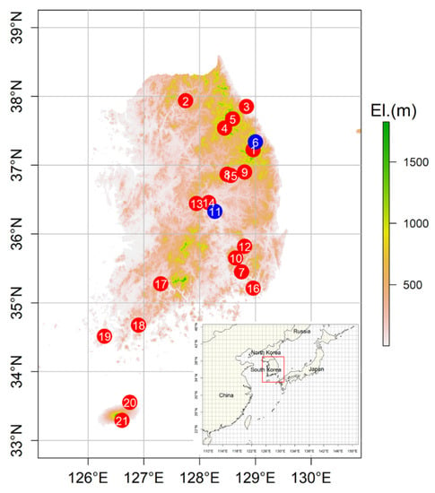
Figure 1.
Locations of selected ground gauge stations for this study. Red and blue circles indicate stations used for raw training and test data sets, respectively.
3. Methods
3.1. Penman–Monteith Model
The PM model was used as a representative model for comparison of the models using satellite observations. The PM model is a physical model that estimates LW based on latent heat flux (LE) that determines the evaporation or condensation of moisture on a surface such as a leaf [9]. The PM model can be applied in any location where the required meteorological observations are available. Sentelhas, et al. [13] reported that the PM model has low spatial variation in various meteorological conditions with good performance and high applicability. Additionally, air temperature observation at the leaf level is unnecessary for PM in estimating LW unlike other physical models that require the estimation of the dew amount and duration. The equation of LE is given as follows:
where s, Rn, es, ea, , ra, and rb are the slope of the saturation vapor pressure curve (hPa), net radiation of the mock leaf (J/min/cm2), saturated vapor pressure at the weather station air temperature (°C), actual air vapor pressure (hPa), modified psychrometer constant (0.64 kPa/K is adopted in the current study), boundary layer resistance for heat transfer, and boundary layer resistance for WS, respectively. The boundary layer resistance for WS, rb, can be calculated as follows:
where D is the effective dimension of the mock leaf (0.07 m in this study). The boundary layer resistance for heat transfer, ra, can be calculated as follows:
where Zs, d, Z0, and WS* are the height of the wetness sensor (m), displacement height (0.5 Zc), roughness length (0.13 Zc), and friction velocity (m/s), respectively. Crop height is represented by Zc (m). For LE estimates at the weather station where the wetness sensor was at the same level as that of the Tair, RH, and WS sensors, the boundary layer resistance for WS was not required in Equation (1). Here, Equation (1) was used to predict LE since the levels of Tair, RH, and WS sensors are different. When LE is greater than zero, the LW is predicted at the specific time. Since net radiation is not observed in the employed sites, they are estimated using the method suggested by Walter, et al. [37]. Since the PM model only considers the condensation of moisture in air near leaf, soil evaporation and transpiration cannot be considered in estimating LW.
3.2. Machine Learning Algorithms
LW prediction involves binary classification of two labels, that is, wetness and dryness, of data. Many ML algorithms were suggested as binary classifiers [38]. We employed logistic regression (LR), ELM, generalized boosted model (GBM), RF, support vector machine (SVM), and deep neural network (DNN) as candidates of classifiers for the LW prediction model. Some ML algorithms such as ELM, RF, and DNN provided good performances for predicting LWD in in-situ meteorological observations [17]. Sixteen channel radiances along with the time of measurement, latitude, and longitude were used as inputs for the ML algorithms. As LW often occurs from dusk to dawn, time is a good input feature. Latitude and longitude were used as these represent geographical characteristics of a target location. The data sets were classified into training, validation, and test data sets for building the ML-based LW prediction model. Observation data sets (8409 data points) of stations #6 and #11 (blue colored circles in Figure 1) were selected as test data sets while those of the other stations (red colored circles in Figure 1) were used as raw training data sets. The raw training data sets were grouped into training and validation data sets. The validation data set comprises of 20,000 (approximate 25% of total data) randomly selected data points out of 79,749 data points and the remaining data points were used as the training data set. The training data set was used to train ML algorithms, and the validation data set was used to optimize hyperparameters of ML algorithms based on the trained algorithms using the training data set. In the training of the ML algorithms, the oversampling strategy was employed to overcome the imbalance in the sample problem, which is, the number of observations showing dryness being much larger than that of wetness. After fixing the hyperparameters of the ML algorithms, the raw training data set was used to train the ML algorithms for building the LW prediction models. Brief descriptions of the employed ML algorithms are presented in the following subsections.
3.2.1. Logistic Regression Model
LR has been broadly used as a classification model [39]. This model provides probabilities of data points belonging to a class using the logistic function. The LR model is expressed as follows:
where , , and b are the probability of a data point belonging to a class, input features, weights, and bias (called intercept), respectively. For regularization, the ridge regression, a technique to penalize the quantity of weights in the regression model using the L1 norm, was adopted in the LR. The weights of the LR using the ridge regression can be obtained as follows:
where , , and n are the label of the data point belonging to a class, tuning parameter, and the number of data points, respectively. The hyperparameter in the LR is the tuning parameter. A small value of the tuning parameter indicates strong regularization in the LR. To optimize the tuning parameter, cross validation is realized using the validation data set. Based on the results obtained, the LR with C = 0.1 leads to the largest accuracy (the number of correct predictions over the number of data points, ACC). Hence, the value of the tuning parameter in the employed LR was 0.1.
3.2.2. Extreme Learning Machine
ELM is a single layer network with randomly generated weights and bias between input and hidden layers [40]. Traditional neural networks need to iteratively optimize weights. Unlike the traditional neural networks, the model can be trained in a single iteration because of the randomized weight and bias. The ELM can be formulized by the following equation:
where , and are the labels, weight matrix between the hidden layer to the output layer, and the output vector of the hidden layer, respectively, and called nonlinear feature mapping.
where , , , and are the activation function, weight matrix between the input layer to the hidden layer, bias, and input feature, respectively. In the current study, the sigmoid function () was used as the activation function in the ELM. Since the weights () and bias () were randomly generated and the activation function () was known in the ELM, was the deterministic variables from a data set. Thus, only needs to be estimated in the ELM.
In the ELM, finding the appropriate weight set to avoid overfitting is important like in an artificial neural network. Tuning weights in the ELM can be considered as fitting a linear regression model using ordinary least squares. Ridge regression is employed to attenuate multicollinearity in the data set by adding a norm of parameters in the parameter estimation of the regression model [41]. The ELM model also adapted this strategy in weight tuning. The ELM attempts to achieve a better generalization performance by reaching not only the smallest training error but also the smallest norm of output weights. This minimization problem can take the form of ridge regression or regularized least squares as [42]:
where the first term of the objective function is l2, a norm regularization term that controls the complexity of the model. The second term is the training error associated with the learned model. C > 0 is a tuning parameter. The ELM gradient equation can be analytically solved, and the closed-form solution can be written as following:
where I is an identity matrix. The regularized ELM model was used in this study. The tuning parameter and the number of hidden nodes are the hyperparameters of ELM. The tuning parameter and number of hidden nodes was systematically tested from 0.5 to 20 and from 100 to 600 for the validation data set, respectively. Based on the results of the cross validation using the validation data set, the ELM model had the largest ACC when the tuning parameter and number of hidden nodes were 10 and 200, respectively. Thus, these two values were employed for the optimal tuning parameter and the number of hidden nodes of the ELM, respectively. Input features were selected via the backward elimination method using the validation data set [43]. Based on the results of the backward elimination method, the ELM model led to the largest ACC when the channels #1, #2, and #7 were removed in the input feature set. The structure of the employed ELM model is presented in Figure 2.
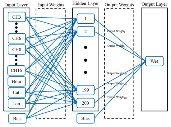
Figure 2.
Structure of the employed extreme learning machine (ELM) model for leaf wetness (LW) prediction.
3.2.3. Random Forest
The RF has been broadly applied for classification problems [44,45]. The RF was proposed by Breiman [46] and uses bagging to build a number of decision trees with controlled variance. Thus, the RF consists of an ensemble of simple decision trees. Each decision tree in the RF is grown using randomly selected samples. Subsequently, the nodes in each tree use randomly selected input features. The RF has two major steps: (1) randomness and (2) ensemble learning.
The randomness in the RF comes from random sampling of the entire data set and the selection of features with which every classification tree is built. The features in the data set are randomly sampled and replaced to create a subset with which to train one classification tree. At each node, the optimal split rule is determined using one of the randomly selected features from the employed features. Approximately two-thirds of the data were selected as the training subset. The features are also randomly selected without being replaced. The data set that is not included in the training subset is denoted as out-of-bag, and it is applied to evaluate the performance of the RF model and the importance of the features.
The ensemble learning method in the RF means that all individual decision trees in a collection of decision trees (called ensemble) contribute to a final prediction. A training subset is created after the random selection step. The classification and regression tree, but without pruning, is used to construct a single decision tree. To grow K number of trees in ensemble, this process (resampling a subset and training individual tree) is repeated K times. The final predicted label is the most frequent label among the predicted labels of all individual trees. The ranger library in the R package was used to construct an RF model [47]. The number of trees was systematically tested from 50 to 600 for the validation data set. Based on the results of the cross validation using the validation data set, the RF with 320 trees led to the largest ACC. Since the RF provides the importance of input features, the input features for the RF were selected based on the importance from the RF with 320 trees. The features were sequentially removed in the input feature set based on the amount of importance until the ACC of the RF decreased. The channel #1, #2, #5, and #6 and longitude were removed in the input feature set for the RF. The structure of the employed RF model is presented in Figure 3.
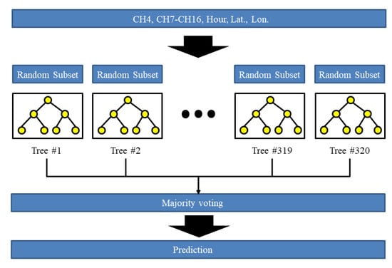
Figure 3.
Structure of the employed random forest (RF) model for LW prediction.
3.2.4. Generalized Boosted Model
The GBM proposed by Friedman [48] is a widely used method in classification problems. Decision stumps or decision trees are used widely as weak classifiers in the GBM [48,49,50]. In the GBM, weak learners are trained to decrease loss functions, e.g., mean square errors. Residuals in the former weak learners are used to train the current weak learners. Therefore, the value of the loss function in the current weak learners decreases. The bagging method is employed to reduce correlation between weak learners, and each weak learner is trained with subsets sampled without replacement from the entire data set. The final prediction is obtained by combining predictions by a set of weak learners.
The GBM and RF adapted ensemble learning with a decision tree model (the weak learner). Both models produce one prediction based on a combination of predictions from a set of weak learners. Though the methods seem to be similar, they are based on different concepts. The major difference between the GBM and RF is that the tree in the GBM is fit on the residual of a subset of the former trees, while the RF trains a set of weak learners using a number of subsets. Therefore, the GBM can reduce the bias of prediction while the RF method can reduce variance of prediction. The gbm library in the R package (https://github.com/gbm-developers/gbm) was used to construct a GBM. The number of trees was systematically tested from 50 to 600 for the validation data set. Based on the results of the cross validation using the validation data set, the GBM with 300 trees leads to the largest ACC. Based on the results of the backward elimination method, the channel #1, #2, #5, and #6 and longitude were removed in the input feature set for the GBM, like in the RF. The structure of the employed GBM model is presented in Figure 4.
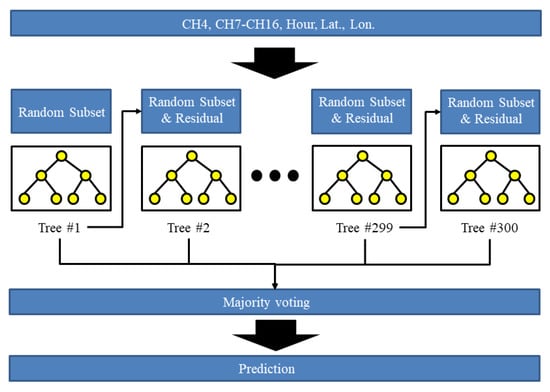
Figure 4.
Structure of the employed generalized boosted model (GBM) for LW prediction.
3.2.5. Support Vector Machine
SVM is applied as a classifier for several classification problems in various fields [51,52,53]. The SVM was developed for solving classification problems based on mathematics unlike other machine learning algorithms such as ELM, RF, and GBM. For example, for linear classification problems, every procedure in the SVM can be proved by a mathematical basis. SVM was developed for building classifiers that maximize the margin, that is, the distance between any two groups. The distance between two groups is determined by the distance between support vectors, that is, the nearest vector to another group. In the current study, ν-SVM was employed for the SVM algorithm [54]. To find the hyperplane for maximizing the margin between the support vectors, the following optimization problem with its constraints needs to be solved.
where , , and are regularization constant that ranges from 0 to 1, slack variable for ith data point, and kernel function that is the radial basis function () in the current study. The ν-SVM for the LW prediction model was implemented using the Scikit-learn in Python [55]. In the ν-SVM, ν is the hyperparameter that represents the tolerance of acceptance for support vectors, which violate the defined hyperplane, and it is optimized by the validation. Value of ν was systematically tested from 0.05 to 1 for validation data set. Based on the validation results, 0.1 was adopted for the value of ν in ν-SVM.
3.2.6. Deep Neural Network
The DNN is a multiple-hidden layer feed-forward network. The main difference between shallow and deep neural networks is the number of hidden layers in the networks. The deep hidden layer of the DNN allows emulating a complex function relation between input and output with the extraction of the complicated feature structure [56]. In the current study, the sigmoid function was used for the activation function of the DNN model. Four hidden layers were adopted for the employed DNN model, and each of these hidden layers has a different number of nodes. The structure of the DNN model was manually optimized because there is no standard method to find the optimal structure. In addition, layer normalization was adopted after second, third, and fourth hidden layers. Layer normalization leads to improvement in the accuracy of the trained DNN model [57]. The structure of the employed DNN model is presented in Figure 5. The Adam algorithm with mini-batch was used to train the DNN model [58]. Pytorch library in python was used to implement the DNN model and train the DNN algorithm. [59]. Size of the mini batch, the number of epochs, and learning rate were set at 3000, 13,000, and 0.0025, respectively. These hyperparameters were manually optimized based on the evaluation of the trained model for the validation data set.
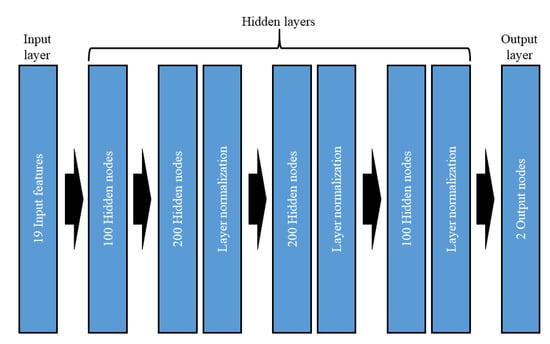
Figure 5.
Structure of the employed deep neural network (DNN) for the LW prediction model.
3.3. Evaluation Measures
To evaluate the performances of the proposed LW prediction models, ACC, recall, precision, and F1 score (F) were employed and calculated as follows:
where TP, TN, FP, and FN indicate the numbers of true positives (correct prediction for wetness), true negatives (correct prediction for dryness), false positives (wrong prediction for wetness), and false negatives (wrong prediction for dryness), respectively. ACC is a proportion between the number of correct predictions from model and total number of predictions. Precision is the fraction of correct predictions among wetness predictions while recall is the fraction of correct prediction among predictions that wetness is observed. For example, when the numbers of predictions for wetness and dryness are 20 and 80 and total number is 200, ACC becomes 0.5 (=100/200). The precision and recall have a tradeoff relationship. Thus, F was suggested to consider precision and recall in evaluating performance of classifier. Root mean square error (RMSE), Pearson correlation (Cor), and mean bias (mBias) are employed as evaluation criteria for the LWD. RMSE is presented as follows:
where, , , and m are ith LWD prediction, ith LWD observation, and the number of data sets, respectively. The Pearson correlation can be calculated as follows:
where, and are means of LWD prediction and observation, respectively. The mBias is given as follows:
where, , , and n are ith LWD prediction, ith LWD observation, and the number of data set, respectively.
4. Results
4.1. Performance Evaluation for LW Prediction Models
The results of the calculations of ACC, recall, precision, and F of LW predictions from all the employed models for the test data are presented in Table 2. Based on the ACC measure, RF shows the best performance in LW prediction among all the employed models including PM that uses in-situ meteorological observations. The GVM, SVM, and DNN models had comparable ACC values to that of the PM. Based on ACC, LR and ELM show poor prediction performances with values less than 0.7.
Table 2.
Evaluation measures of all the employed LW prediction models for the test data set. Note that the underlined numbers indicate the best performance based on the employed evaluation measure.
Although ACC is often employed as the main performance evaluation measure of classification models, it has limited performance when there is imbalance in the data set. In such a situation, F is an alternative to evaluate the performance of the classification model, as it is a hybrid measure that combines recall and precision. The F values of the ML-based LW prediction models were lower than that of PM. Values of F for LR, GBM, and SVM were lower than 0.4. Although the ACCs of GBM and SVM were relatively high among the tested models, their Fs were very low. Since the proportion of dryness was approximately 80%, the ACC of a model had 0.8 when it only returned dryness. Hence, this result indicates that GBM and SVM overestimated dryness. Overall, the prediction performance of LR was the poorest among the models based on the evaluation measures.
The ELM, RF, and DNN models provided comparable F to PM. The values of the recall for ELM and RF were much lower than that of PM while these models led to high precision. Particularly, LW predictions by RF show the largest precision. These results mean that the wetness predicted by ELM and RF had high accuracy, but their performances in its detection were limited. The DNN model provided LW prediction with the largest recall while the value of its precision was very low. The DNN detected wetness but its prediction was inaccurate. These results show that some ML-based LW models provided a prediction performance comparable to that of the PM even though the PM slightly outperformed them. The results of evaluating performance of LW models indicate that the LW prediction using satellite observation and ML algorithm would be an alternative.
4.2. Performance Evaluation for LWD Predictions
The performances of the employed models for predicting LWD were evaluated using RMSE, Cor, and mBias for the test data set; these values are listed in Table 3. The PM had the smallest RMSE between the predicted and observed LWD among all the employed models for the test data set followed by DNN and RF. Based on the Cor, the DNN had the best performance followed by RF and PM. Overall, PM, RF, and DNN provided superior performances in predicting LWD. To investigate the prediction performances of PM, LR, SVM, GVM, RF, and DNN in detail, the density plots of LWD predictions and observations were made and they are shown in Figure 6. The data points having zero values in both prediction and observation were excluded to highlight the other values of LWD since the number of data with zero values was much larger than the number of other data points. Since ELM had the largest RMSE in Table 3, it was excluded from the density plots. Figure 6a shows that the LWD predictions by the PM were scattered around a diagonal line. Overestimation of the LWD predictions was presented by LR and DNN while underestimation was observed in RF, GBM, and SVM. The Cor values, after excluding data points having zeros in both prediction and observation, show that the DNN and RF would provide more accurate LWD predictions than that of the PM. The RMSE of DNN presented in Figure 6 was smaller than that of the PM. These results indicate that RF and DNN provide good performances in LWD prediction that are comparable to that of the PM.
Table 3.
Evaluation measures of all the employed LWD prediction models for all stations in the test data set. Note that the underlined numbers indicate the best performance based on the employed evaluation measures.
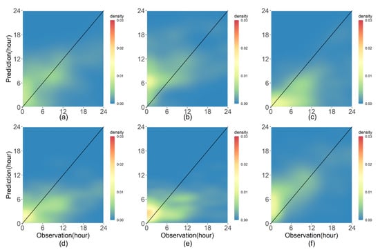
Figure 6.
Density plots for leaf wetness duration (LWD) models based on (a) Penman–Monteith (PM; Cor: 0.508, root mean square error (RMSE): 5.805 h), (b) logistic regression (LR; Cor: 0.421, RMSE: 7.004 h), (c) RF (Cor: 0.569, RMSE: 6.791 h), (d) GBM (Cor: 0.481, RMSE: 6.436 h), (e) support vector machine (SVM; Cor: 0.376, RMSE: 6.268 h), and (f) DNN (Cor: 0.703, RMSE: 5.209 h) for all the stations in the test data set excluding the data points having zero values in both prediction and observation. Note that the Cor and RMSE were calculated from the test data set excluding the data points having zero values.
Since the LWD is a local phenomenon, investigating the prediction performance of the employed models with respect to the individual station or at the local scale is important. Hence, the evaluation measures for each station (stations #6 and #11) using the test data set were calculated and presented in Table 4.
Table 4.
Evaluation measures of all the employed LWD models for individual stations using the test data set. Note that the underlined numbers indicate the best performance based on the employed evaluation measures.
For station #6, PM and DNN provided similar prediction performances based on RMSE and Cor. Though the RF shows a better performance than LR, it was worse than PM and DNN. For station #11, RF had the best performance among the employed models. RMSE and Cor of the LWD predictions by RF were 3.67 h and 0.815, respectively. Particularly, RF had a better performance than PM that used in-situ meteorological variables for LWD prediction. The DNN also shows good performance, and it was competitive to PM. Although the results of the individual stations were consistent with the results of all the stations for the test data set, the prediction performances of the employed models varied with the local characteristics. To investigate the detailed characteristics of LWD predictions at the local scale, the density plots of the PM, LR, SVM, GVM, RF, and DNN were made for stations #6 and #11 and they are presented in Figure 7 and Figure 8, respectively.
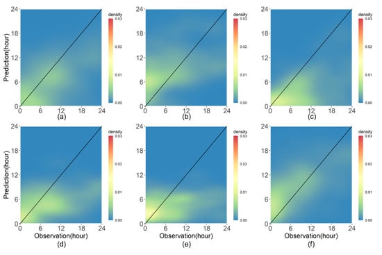
Figure 7.
Density plots for LWD models based on (a) PM (Cor: 0.560, RMSE: 6.439 h), (b) LR (Cor: 0.450, RMSE: 6.774 h), (c) RF (Cor: 0.504, RMSE: 7.976 h), (d) GBM (Cor: 0.457, RMSE: 6.96 h), (e) SVM (Cor: 0.254, RMSE: 7.391 h), and (f) DNN (Cor: 0.667, RMSE: 5.572 h) for station #6 in the test data set excluding the data points having zero values in both prediction and observation. Note that the Cor and RMSE were calculated from the test data set excluding the data points having zero values.

Figure 8.
Density plots for LWD models based on (a) PM (Cor: 0.587, RMSE: 5.129 h), (b) LR (Cor: 0.422, RMSE: 7.226 h), (c) RF (Cor: 0.718, RMSE: 4.847 h), (d) GBM (Cor: 0.467, RMSE: 5.737 h), (e) SVM (Cor: 0.503, RMSE: 4.866 h), and (f) DNN (Cor: 0.741, RMSE: 4.817 h) for station #11 in the test data set excluding the data points having zero values in both prediction and observation. Note that the Cor and RMSE were calculated from the test data set excluding the data points having zero values.
Figure 7 and Figure 8 show that the overall characteristics of the LWD predictions for the employed models were similar to those in Figure 6. Overestimation of LWD predictions is presented in LR and DNN while underestimation was observed in RF, GBM, and SVM. For station #6, the RF provided a strong underestimation while the DNN led to a small overestimation. For station #11, the PM seemed to overestimate LWD. Though the RF led to underestimation, the magnitude of underestimation was weaker than that for station #6. Unlike in the case of RF, overestimation by DNN became stronger in station #6.
Only the test data sets pertaining to the two stations were analyzed because of limited data availability. Dates that had a larger number of data points were only selected to evaluate the performance of the employed models for spatial distribution of LWD prediction as otherwise the generality of the evaluation can be lost. Four days from 1 March 2020 to 4 March 2020 were chosen. In this period, the LWD observations from 60 stations that were not used for raw training or as test data sets could be used for evaluation. The RMSEs of the LWD predictions by the PM, RF, and DNN for the 60 employed stations were 5.2 h, 3.4 h, and 9.1 h, respectively. Based on the RMSE, the RF shows the best performance for LWD prediction during this period. The biases of the PM, RF, and DNN were 3.2 h, 1.3 h, and 8.2 h, respectively. The models, PM, RF, and DNN had positive biases, and the bias of the DNN model was very large. The poor performance of the DNN was attributed to its large positive bias. The spatial distributions of LWD predictions of RF and DNN for the selected date are presented in Figure 9 to investigate their characteristics. Figure 9 shows that the values of LWD by DNN were much larger than those of RF. The overall patterns of spatial distributions of LWD by RF and DNN were dissimilar. The result indicates that the LWD prediction models could have a large discrepancy although the differences between the performances of the employed models were small based on the results of the evaluation measures. Overall, the LWD prediction model using the RF and satellite observation may be a good alternative to predict LWD in ungauged locations and obtain consistent quality of LWD prediction.
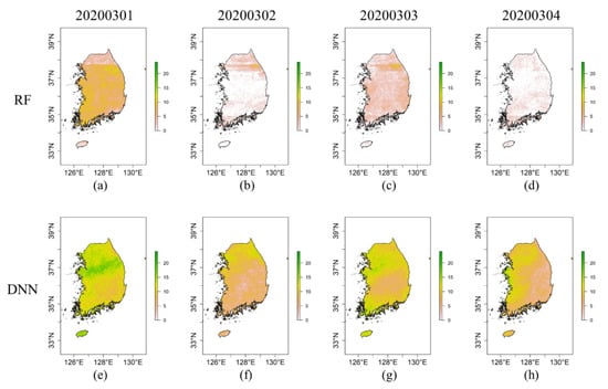
Figure 9.
Spatial distribution of LWD predictions of RF and DNN from 1 March 2020 to 4 March 2020: (a) RF at 1 March 2020, (b) RF at 2 March 2020, (c) RF at 3 March 2020, (d) RF at 4 March 2020, (e) DNN at 1 March 2020, (f) DNN at 2 March 2020, (g) DNN at 3 March 2020, and (h) DNN at 4 March 2020.
5. Discussion
The results of the study show that satellite observations can be used for LWD prediction. The RF model exhibited the best performance in LW prediction and a good performance in LWD prediction using satellite observations. The DNN model also provided a good performance in LWD prediction. Based on the results of the performance evaluation for the spatial distribution of LWD, RF showed the most accurate prediction although only snapshots of LWD observations were used in the evaluation process. Overall, the PM was the best LWD prediction model among all the employed models because it was among the best three models in all evaluation results. Notably, the values of recall and precision in LW prediction were higher than 0.5 for PM. Despite its superiority, PM cannot predict LWD in an ungauged location since in-situ meteorological data are required. Unlike PM, the other LWD prediction models proposed in the current study can make predictions in an ungauged location because they can use satellite observations. However, because PM can consider local meteorological characteristics, its superiority among the employed models was established. Although the PM had an advantage in terms of performance evaluation, the other LWD prediction models produced accurate LWD predictions that were comparable to that of the PM. Therefore, LWD prediction models that use satellite observations have the potential to predict LWD in locations where in-situ meteorological data is unavailable.
As listed in Table 1, each channel had a different set of physical properties. Investigating the specific influence of a channel on LWD prediction is critical in understanding the relationship between satellite and LWD observations. The RF model can provide the importance of input features in predicting a variable of interest [17]. Here, importance means the magnitude of decrease in the accuracy of the model when the selected input feature is not used in it. The RF model randomly selects input features and samples data for building a single decision tree, and therefore, some input features and data are not used in the training. By using the unused data, the importance of the input features can be calculated. As RF emerged as one of the good models for predicting LWD, investigating the importance of input features would establish the relationship between satellite and LWD observations. Figure 10 presents the importance of the input features from RF for the raw training data set. The results of the importance evaluation of RF show that channels #1 to #6 have a much lower importance than those of channels #7 to #16. The LWD is often generated at dawn and nighttime. As longwave channels can observe radiance at nighttime, these channels would provide critical information for predicting LWD. The most important channel was channel #7 as it can represent low cloud, fog, fire, and wind, which are important components for LWD prediction accounting for most of the generating mechanisms of LW. Furthermore, the channel #7 would detect the changes in radiance at dawn because it is a mid-infrared channel. Due to these characteristics, this channel may successfully deliver information for predicting LWD. The second most important channel was channel #12, which can represent the total ozone, turbulence, and wind. The channels that can represent critical meteorological variables such as humidity, solar radiation, wind speed, and temperature in LWD have high values of importance and so do related longwave channels. These results suggest that the use of mid- and longwave channels would be beneficial in LWD prediction.
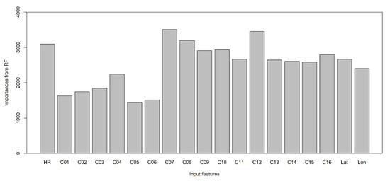
Figure 10.
Importance of input features from RF for the raw training data set.
The results of this study may not represent the typical characteristics of LWD because the observation data only cover two seasons: winter and spring. The generating mechanisms of LW varied with the seasons, for instance, LW in summer was often caused by rainfall, while the condensation of water vapor on the leaf (dew) caused LW in winter. In addition, the frequency of LW varied with seasons. The proportion of LW observations used in this study was 80%. When the LW observations in summer were included, the proportion would be approximately 60%. To generalize results based on the performance evaluation for LWD prediction using satellite observations, a longer period is required. Hence, the results of the performance evaluation in the current study were indicative and not definitive in deciding the most appropriate model for LWD prediction using satellite observations. All the considered models for LWD prediction will be extensively compared in a future study. More input features providing local information, e.g., geographic, phenological, and vegetation information, are required to improve the performance of the LWD prediction model. Some channels may approximately reflect geographic and phenological information for the area of interest. Spatial resolution of the satellite observations is too coarse to describe the local geographic and phenological information. Due to this limitation, the proposed models may have limited performances. If this information can be integrated in the model for predicting LWD, its accuracy will be improved. A LWD prediction model using satellite observation based on physics should be developed to obtain a consistent prediction with large meteorological variations. The approach proposed in the current study may provide different results for other regions or countries because ML algorithms are employed as a classifier in building the LW prediction model using satellite observations. Results may also vary depending on the use of different products from different satellites. The main advantage of a physics-based LWD prediction model, e.g., PM, is that the model can be used in any region [13]. Standard protocols for measuring LWD and maintaining instruments are required to obtain reliable observations and expand their coverage. As shown in Figure 1, the northwestern region of South Korea is not represented in this study. Once a standard protocol is prepared, LWD observations of some stations in this area can be used. This will lead to an increase in coverage and a better performance of LWD prediction.
The ML algorithm can provide unrealistic results even if the LWD prediction model is properly developed. For example, the LWD prediction model using DNN shows good performance based on evaluation measures. In Figure 9, the LWD prediction model using DNN overestimated LWD for all tested days. In addition, stripe noise from the satellite images was amplified by RF in LWD prediction. Though the stripe noise in satellite images is inevitable, they can be reduced by noise filtering algorithms [60,61,62]. Strong stripe noise was not overserved raw satellite images. However, clear stripe noise appeared in Figure 9a–d. This result implies that application of the ML algorithms can amply stripe noise in the satellite images. Thus, when the LWD prediction model using ML algorithm is considered in the operational system, robustness of the prediction model should be thoroughly inspected for various cases in order to attenuate the possibility of having a wrong prediction.
6. Conclusions
An approach to obtain LWD prediction using satellite data and ML algorithms as classifiers was proposed. The feasibility of the proposed approach was evaluated using satellite data (GK-2A) and ML algorithms in South Korea through different models that showed good performances. Performance evaluation of the models showed that the performances of the proposed models in predicting LWD were comparable to that of PM. The proposed models can be utilized to obtain LWD data for locations in which meteorological instruments are not installed. Among the prediction models, RF and DNN showed good performances in predicting LWD in South Korea. These two ML algorithms can be used as classifiers in building an LWD prediction model using satellite observations in other regions. The applicability of satellite observations in LWD prediction needs further improvements. For example, integrating local information such as elevation and vegetation types in the LWD prediction model may improve its performance. Additionally, ML algorithms may perform poorly when data sets with different meteorological characteristics are used as inputs. Therefore, a physics-based LWD prediction model using satellite observations should be developed through future research.
Author Contributions
Conceptualization, J.-Y.S., K.R.K., J.P., J.W.C., and B.-Y.K.; methodology, J.-Y.S., K.R.K. and B.-Y.K.; software, J.-Y.S.; validation, J.-Y.S., K.R.K. and B.-Y.K.; formal analysis, J.-Y.S.; investigation, K.R.K. and J.W.C.; resources, K.R.K. and J.W.C.; data curation, J.P. and B.-Y.K.; writing—original draft preparation, J.-Y.S. and B.-Y.K.; writing—review and editing, J.-Y.S., K.R.K., J.W.C., and B.-Y.K.; visualization, J.-Y.S.; supervision, K.R.K.; project administration, K.R.K.; funding acquisition, K.R.K. All authors have read and agreed to the published version of the manuscript.
Funding
This work was funded by the Korea Meteorological Administration Research and Development Program “Advanced Research on Biometeorology” under Grant (KMA2018-00620).
Acknowledgments
This work was funded by the Korea Meteorological Administration Research and Development Program “Advanced Research on Biometeorology” under Grant (KMA2018-00620).
Conflicts of Interest
The authors declare no conflict of interest.
References
- Magarey, R.D.; Russo, J.M.; Seem, R.C.; Gadoury, D.M. Surface wetness duration under controlled environmental conditions. Agric. For. Meteorol. 2005, 128, 111–122. [Google Scholar] [CrossRef]
- Huber, L.; Gillespie, T.J. Modeling Leaf Wetness in Relation to Plant Disease Epidemiology. Annu. Rev. Phytopathol. 1992, 30, 553–577. [Google Scholar] [CrossRef]
- Schmitz, H.F.; Grant, R.H. Precipitation and dew in a soybean canopy: Spatial variations in leaf wetness and implications for Phakopsora pachyrhizi infection. Agric. For. Meteorol. 2009, 149, 1621–1627. [Google Scholar] [CrossRef]
- Rowlandson, T.; Gleason, M.; Sentelhas, P.; Gillespie, T.; Thomas, C.; Hornbuckle, B. Reconsidering Leaf Wetness Duration Determination for Plant Disease Management. Plant. Dis. 2015, 99, 310–319. [Google Scholar] [CrossRef] [PubMed]
- Gleason, M.L.; Duttweiler, K.B.; Batzer, J.C.; Taylor, S.E.; Sentelhas, P.C.; Monteiro, J.E.B.A.; Gillespie, T.J. Obtaining weather data for input to crop disease-warning systems: Leaf wetness duration as a case study. Scientia Agricola 2008, 65, 76–87. [Google Scholar] [CrossRef]
- Miranda, R.A.C.; Davies, T.D.; Cornell, S.E. A laboratory assessment of wetness sensors for leaf, fruit and trunk surfaces. Agric. For. Meteorol. 2000, 102, 263–274. [Google Scholar] [CrossRef]
- Sentelhas, P.C.; Gillespie, T.J.; Gleason, M.L.; Monteiro, J.E.B.A.; Helland, S.T. Operational exposure of leaf wetness sensors. Agric. For. Meteorol. 2004, 126, 59–72. [Google Scholar] [CrossRef]
- Sentelhas, P.C.; Gillespie, T.J.; Santos, E.A. Leaf wetness duration measurement: Comparison of cylindrical and flat plate sensors under different field conditions. Int. J. Biometeorol. 2007, 51, 265–273. [Google Scholar] [CrossRef]
- Rao, P.S.; Gillespie, T.J.; Schaafsma, A.W. Estimating wetness duration on maize ears from meteorological observations. Can. J. Soil. Sci. 1998, 78, 149–154. [Google Scholar] [CrossRef]
- Kim, K.S.; Taylor, S.E.; Gleason, M.L.; Koehler, K.J. Model to Enhance Site-Specific Estimation of Leaf Wetness Duration. Plant. Dis. 2002, 86, 179–185. [Google Scholar] [CrossRef]
- Papastamati, K.; McCartney, H.A.; Bosch, F.V.D. Modelling leaf wetness duration during the rosette stage of oilseed rape. Agric. For. Meteorol. 2004, 123, 69–78. [Google Scholar] [CrossRef]
- Leca, A.; Parisi, L.; Lacointe, A.; Saudreau, M. Comparison of Penman-Monteith and non-linear energy balance approaches for estimating leaf wetness duration and apple scab infection. Agric. For. Meteorol. 2011, 151, 1158–1162. [Google Scholar] [CrossRef]
- Sentelhas, P.C.; Gillespie, T.J.; Gleason, M.L.; Monteiro, J.E.B.M.; Pezzopane, J.R.M.; Pedro, M.J. Evaluation of a Penman–Monteith approach to provide “reference” and crop canopy leaf wetness duration estimates. Agric. For. Meteorol. 2006, 141, 105–117. [Google Scholar] [CrossRef]
- Francl, L.J.; Panigrahi, S. Artificial neural network models of wheat leaf wetness. Agric. For. Meteorol. 1997, 88, 57–65. [Google Scholar] [CrossRef]
- Kim, K.S.; Taylor, S.E.; Gleason, M.L. Development and validation of a leaf wetness duration model using a fuzzy logic system. Agric. For. Meteorol. 2004, 127, 53–64. [Google Scholar] [CrossRef]
- Marta, A.D.; De Vincenzi, M.; Dietrich, S.; Orlandini, S. Neural network for the estimation of leaf wetness duration: Application to a Plasmopara viticola infection forecasting. Phys. Chem. Earth 2005, 30, 91–96. [Google Scholar] [CrossRef]
- Park, J.; Shin, J.-Y.; Kim, K.R.; Ha, J.-C. Leaf Wetness Duration Models Using Advanced Machine Learning Algorithms: Application to Farms in Gyeonggi Province, South Korea. Water 2019, 11, 1878. [Google Scholar] [CrossRef]
- Wang, H.; Sanchez-Molina, J.A.; Li, M.; Rodríguez Díaz, F. Improving the Performance of Vegetable Leaf Wetness Duration Models in Greenhouses Using Decision Tree Learning. Water 2019, 11, 158. [Google Scholar] [CrossRef]
- Wagle, P.; Bhattarai, N.; Gowda, P.H.; Kakani, V.G. Performance of five surface energy balance models for estimating daily evapotranspiration in high biomass sorghum. ISPRS J. Photogramm. 2017, 128, 192–203. [Google Scholar] [CrossRef]
- Kim, B.-Y.; Lee, K.-T.; Jee, J.-B.; Zo, I.-S. Retrieval of outgoing longwave radiation at top-of-atmosphere using Himawari-8 AHI data. Remote Sens. Environ. 2018, 204, 498–508. [Google Scholar] [CrossRef]
- Kim, B.-Y.; Lee, K.-T. Radiation Component Calculation and Energy Budget Analysis for the Korean Peninsula Region. Remote Sens. 2018, 10, 1147. [Google Scholar] [CrossRef]
- Khand, K.; Taghvaeian, S.; Gowda, P.; Paul, G. A Modeling Framework for Deriving Daily Time Series of Evapotranspiration Maps Using a Surface Energy Balance Model. Remote Sens. 2019, 11, 508. [Google Scholar] [CrossRef]
- Ryu, H.-S.; Hong, S. Sea Fog Detection Based on Normalized Difference Snow Index Using Advanced Himawari Imager Observations. Remote Sens. 2020, 12, 1521. [Google Scholar] [CrossRef]
- Cho, J.; Lee, Y.-W.; Han, K.-S. The effect of fractional vegetation cover on the relationship between EVI and soil moisture in non-forest regions. Remote Sens. Lett. 2014, 5, 37–45. [Google Scholar] [CrossRef]
- Lee, C.S.; Park, J.D.; Shin, J.; Jang, J. Improvement of AMSR2 Soil Moisture Products Over South Korea. IEEE J. Sel. Top. Appl. Earth Obs. Remote Sens. 2017, 10, 3839–3849. [Google Scholar] [CrossRef]
- Cho, J.; Lee, Y.-W.; Lee, H.-S. Assessment of the relationship between thermal-infrared-based temperature−vegetation dryness index and microwave satellite-derived soil moisture. Remote Sens. Lett. 2014, 5, 627–636. [Google Scholar] [CrossRef]
- Kwon, Y.-J.; Ryu, S.; Cho, J.; Lee, Y.-W.; Park, N.-W.; Chung, C.-Y.; Hong, S. Infrared Soil Moisture Retrieval Algorithm Using Temperature-Vegetation Dryness Index and Moderate Resolution Imaging Spectroradiometer Data. Asia-Pac. J. Atmos. Sci. 2020, 56, 275–289. [Google Scholar] [CrossRef]
- Kim, K.S.; Hill, G.N.; Beresford, R.M. Remote sensing and interpolation methods can obtain weather data for disease prediction. N.Z. Plant Prot. 2010, 63, 182–186. [Google Scholar] [CrossRef]
- Cosh, M.H.; Kabela, E.D.; Hornbuckle, B.; Gleason, M.L.; Jackson, T.J.; Prueger, J.H. Observations of dew amount using in situ and satellite measurements in an agricultural landscape. Agric. For. Meteorol. 2009, 149, 1082–1086. [Google Scholar] [CrossRef]
- Kabela, E.D.; Hornbuckle, B.K.; Cosh, M.H.; Anderson, M.C.; Gleason, M.L. Dew frequency, duration, amount, and distribution in corn and soybean during SMEX05. Agric. For. Meteorol. 2009, 149, 11–24. [Google Scholar] [CrossRef]
- Anderson, M.C.; Bland, W.L.; Norman, J.M.; Diak, G.D. Canopy Wetness and Humidity Prediction Using Satellite and Synoptic-Scale Meteorological Observations. Plant Disease 2001, 85, 1018–1026. [Google Scholar] [CrossRef]
- Choi, Y.-S.; Ho, C.-H. Earth and environmental remote sensing community in South Korea: A review. Remote Sens. Appl. Soc. Environ. 2015, 2, 66–76. [Google Scholar] [CrossRef]
- Schmit, T.J.; Gunshor, M.M.; Menzel, W.P.; Gurka, J.J.; Li, J.; Bachmeier, A.S. Introducing the next-generation advanced baseline imager on GOES-R. Bull. Am. Meteorol. Soc. 2005, 86, 1079–1096. [Google Scholar] [CrossRef]
- Oh, S.M.; Borde, R.; Carranza, M.; Shin, I.-C. Development and Intercomparison Study of an Atmospheric Motion Vector Retrieval Algorithm for GEO-KOMPSAT-2A. Remote Sens. 2019, 11, 2054. [Google Scholar] [CrossRef]
- Park, K.-A.; Woo, H.-J.; Chung, S.-R.; Cheong, S.-H. Development of Sea Surface Temperature Retrieval Algorithms for Geostationary Satellite Data (Himawari-8/AHI). Asia-Pac. J. Atmos. Sci. 2020, 56, 187–206. [Google Scholar] [CrossRef]
- Sentelhas, P.C.; Dalla Marta, A.; Orlandini, S.; Santos, E.A.; Gillespie, T.J.; Gleason, M.L. Suitability of relative humidity as an estimator of leaf wetness duration. Agric. For. Meteorol. 2008, 148, 392–400. [Google Scholar] [CrossRef]
- Walter, I.A.; Allen, R.G.; Elliott, R.; Jensen, M.E.; Itenfisu, D.; Mecham, B.; Howel, T.A.; Snyder, R.; Brown, P.; Echings, S.; et al. ASCE’s Standardized Reference Evapotranspiration Equation. In Watershed Management and Operations Management; ASCE: Reston, VA, USA, 2000; pp. 1–11. [Google Scholar]
- Holloway, J.; Mengersen, K. Statistical Machine Learning Methods and Remote Sensing for Sustainable Development Goals: A Review. Remote Sens. 2018, 10, 1365. [Google Scholar] [CrossRef]
- Van Houwelingen, J.C.; le Cessie, S. Logistic Regression, a review. Stat. Neerl. 1988, 42, 215–232. [Google Scholar] [CrossRef]
- Huang, G.-B.; Zhu, Q.-Y.; Siew, C.-K. Extreme learning machine: Theory and applications. Neurocomputing 2006, 70, 489–501. [Google Scholar] [CrossRef]
- Peña, M.; Dool, H.V.D. Consolidation of Multimodel Forecasts by Ridge Regression: Application to Pacific Sea Surface Temperature. J. Clim. 2008, 21, 6521–6538. [Google Scholar] [CrossRef]
- Huang, G.; Zhou, H.; Ding, X.; Zhang, R. Extreme Learning Machine for Regression and Multiclass Classification. IEEE Trans. Syst. Man Cybern. B Cybern. 2012, 42, 513–529. [Google Scholar] [CrossRef] [PubMed]
- Xu, L.; Zhang, W.-J. Comparison of different methods for variable selection. Anal. Chim. Acta 2001, 446, 475–481. [Google Scholar] [CrossRef]
- Pal, M. Random forest classifier for remote sensing classification. Int. J. Remote. Sens. 2005, 26, 217–222. [Google Scholar] [CrossRef]
- Smith, A. Image segmentation scale parameter optimization and land cover classification using the Random Forest algorithm. J. Spat. Sci. 2010, 55, 6979. [Google Scholar] [CrossRef]
- Breiman, L. Random Forests. Mach. Learn. 2001, 45, 5–32. [Google Scholar] [CrossRef]
- Wright, M.N.; Ziegler, A. Ranger: A Fast Implementation of Random Forests for High Dimensional Data in C++ and R. J. Stat. Softw. 2017, 77, 17. [Google Scholar] [CrossRef]
- Friedman, J.H. Stochastic gradient boosting. Comput. Statist. Data Anal. 2002, 38, 367–378. [Google Scholar] [CrossRef]
- Naghibi, S.A.; Pourghasemi, H.R.; Dixon, B. GIS-based groundwater potential mapping using boosted regression tree, classification and regression tree, and random forest machine learning models in Iran. Environ. Monit. Assess. 2016, 188, 44. [Google Scholar] [CrossRef] [PubMed]
- Torres-Barrán, A.; Alonso, Á.; Dorronsoro, J.R. Regression tree ensembles for wind energy and solar radiation prediction. Neurocomputing 2019, 326–327, 151–160. [Google Scholar] [CrossRef]
- Shrestha, N.K.; Shukla, S. Support vector machine based modeling of evapotranspiration using hydro-climatic variables in a sub-tropical environment. Agric. For. Meteorol. 2015, 200, 172–184. [Google Scholar] [CrossRef]
- Yao, Y.; Liang, S.; Li, X.; Chen, J.; Liu, S.; Jia, K.; Zhang, X.; Xiao, Z.; Fisher, J.B.; Mu, Q.; et al. Improving global terrestrial evapotranspiration estimation using support vector machine by integrating three process-based algorithms. Agric. For. Meteorol. 2017, 242, 55–74. [Google Scholar] [CrossRef]
- Jung, K.; Shin, J.-Y.; Park, D. A new approach for river network classification based on the beta distribution of tributary junction angles. J. Hydrol. 2019, 572, 66–74. [Google Scholar] [CrossRef]
- Chen, P.-H.; Lin, C.-J.; Schölkopf, B. A tutorial on ν-support vector machines. Appl. Stoch. Model. Bus. 2005, 21, 111–136. [Google Scholar] [CrossRef]
- Pedregosa, F.; Varoquaux, G.; Gramfort, A.; Michel, V.; Thirion, B.; Grisel, O.; Blondel, M.; Prettenhofer, P.; Weiss, R.; Dubourg, V. Scikit-learn: Machine learning in Python. J. Mach. Learn. Res. 2011, 12, 2825–2830. [Google Scholar]
- Tao, Y.; Gao, X.; Hsu, K.; Sorooshian, S.; Ihler, A. A Deep Neural Network Modeling Framework to Reduce Bias in Satellite Precipitation Products. J. Hydrometeorol. 2016, 17, 931–945. [Google Scholar] [CrossRef]
- Xu, J.; Sun, X.; Zhang, Z.; Zhao, G.; Lin, J. Understanding and Improving Layer Normalization. Proceedings of the Advances in Neural Information Processing Systems, USA; 2019, pp. 4381–4391. Available online: https://deepai.org/publication/understanding-and-improving-layer-normalization (accessed on 3 September 2020).
- Kingma, D.P.; Ba, J. Adam: A method for stochastic optimization. arXiv Preprint 2014, arXiv:1412.6980. [Google Scholar]
- Paszke, A.; Gross, S.; Massa, F.; Lerer, A.; Bradbury, J.; Chanan, G.; Killeen, T.; Lin, Z.; Gimelshein, N.; Antiga, L. Pytorch: An Imperative Style, High-Performance Deep Learning Library. In Proceedings of the Advances in Neural Information Processing Systems, USA; 2019; pp. 8026–8037. Available online: https://papers.nips.cc/paper/9015-pytorch-an-imperative-style-high-performance-deep-learning-library (accessed on 1 September 2020).
- Rakwatin, P.; Takeuchi, W.; Yasuoka, Y. Stripe Noise Reduction in MODIS Data by Combining Histogram Matching With Facet Filter. IEEE Trans. Geosci. Remote Sens. 2007, 45, 1844–1856. [Google Scholar] [CrossRef]
- Münch, B.; Trtik, P.; Marone, F.; Stampanoni, M. Stripe and ring artifact removal with combined wavelet Fourier filtering. Opt. Express 2009, 17, 8567–8591. [Google Scholar] [CrossRef]
- Shen, H.; Zhang, L. A MAP-Based Algorithm for Destriping and Inpainting of Remotely Sensed Images. IEEE Trans. Geosci. Remote Sens. 2009, 47, 1492–1502. [Google Scholar] [CrossRef]
© 2020 by the authors. Licensee MDPI, Basel, Switzerland. This article is an open access article distributed under the terms and conditions of the Creative Commons Attribution (CC BY) license (http://creativecommons.org/licenses/by/4.0/).