Continuous Forest Monitoring Using Cumulative Sums of Sentinel-1 Timeseries


Abstract
1. Introduction
Detecting Forest Changes With Pairwise Analysis of SAR Data
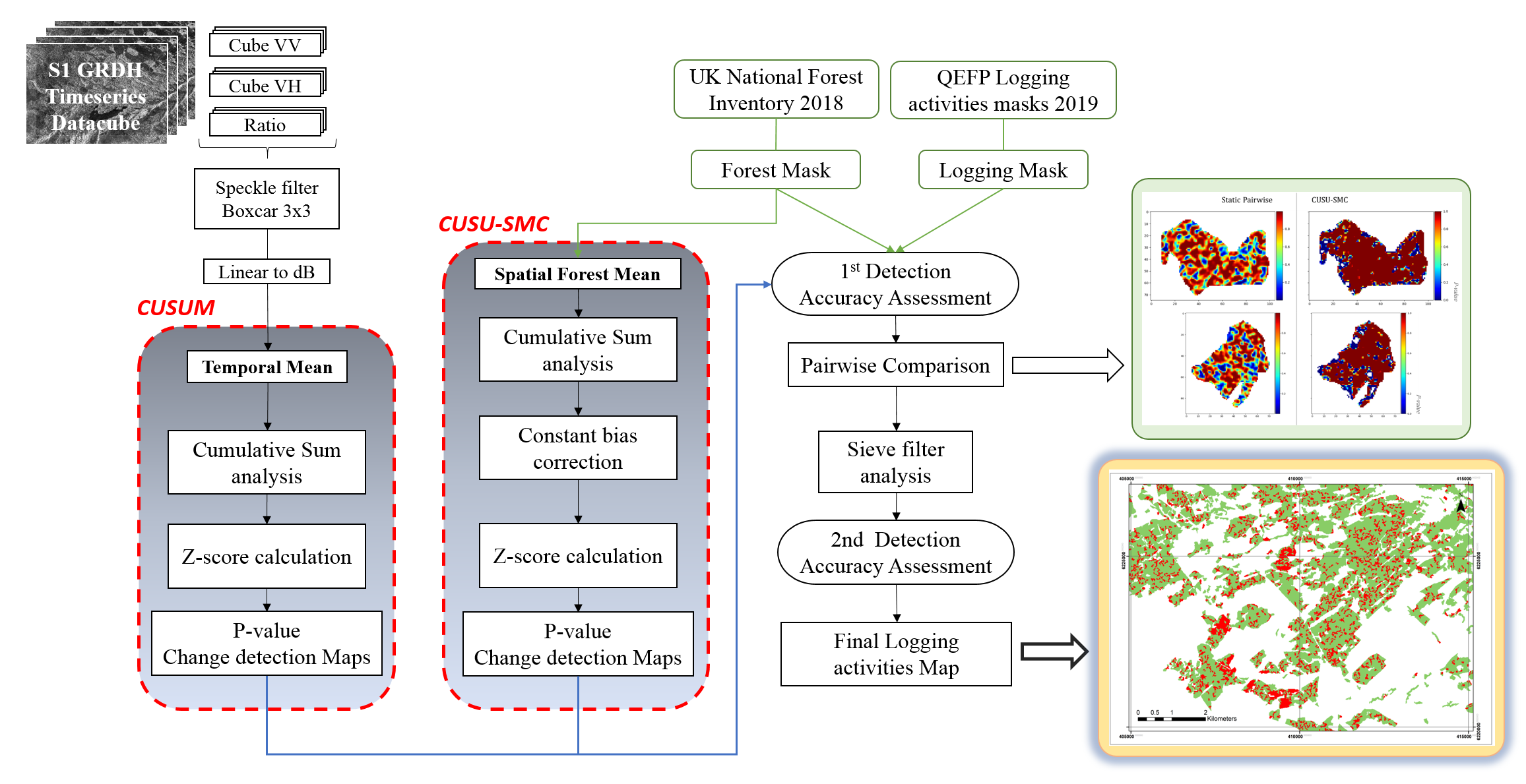
2. Study Area
3. Materials
3.1. SAR Data
3.2. SAR Data Pre-Processing
3.3. Validation Data: Forest Mask and Logging Activities Reference Data
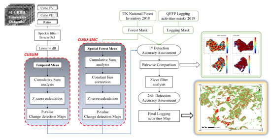
4. Methodologies
4.1. Cumulative Sum Change Detection Analysis
4.2. CUSU-SMC
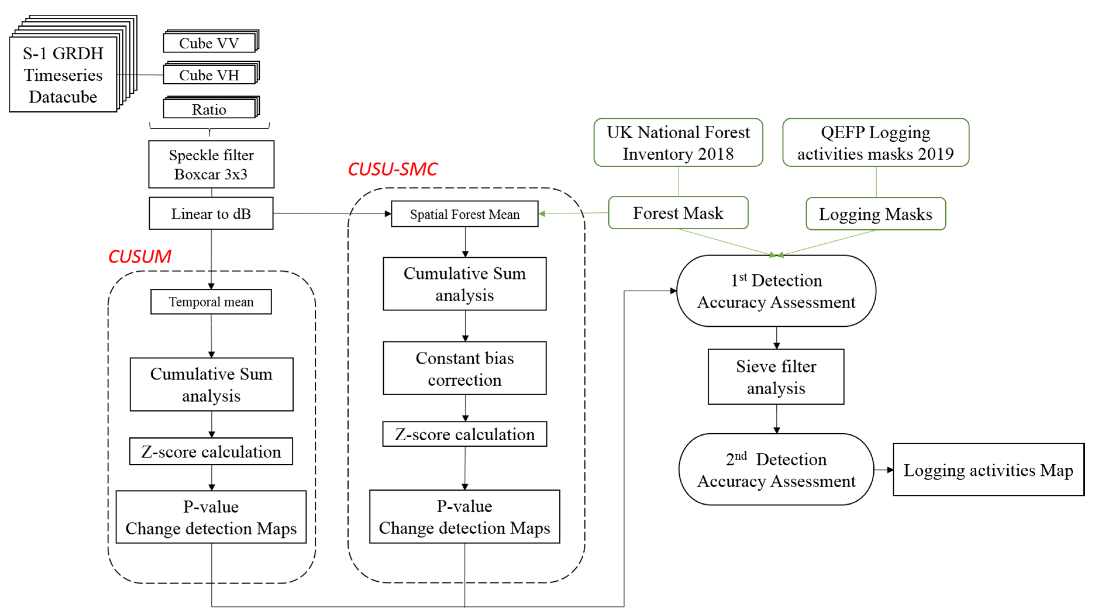
4.3. CUSU-SMC Implementation
- (1)
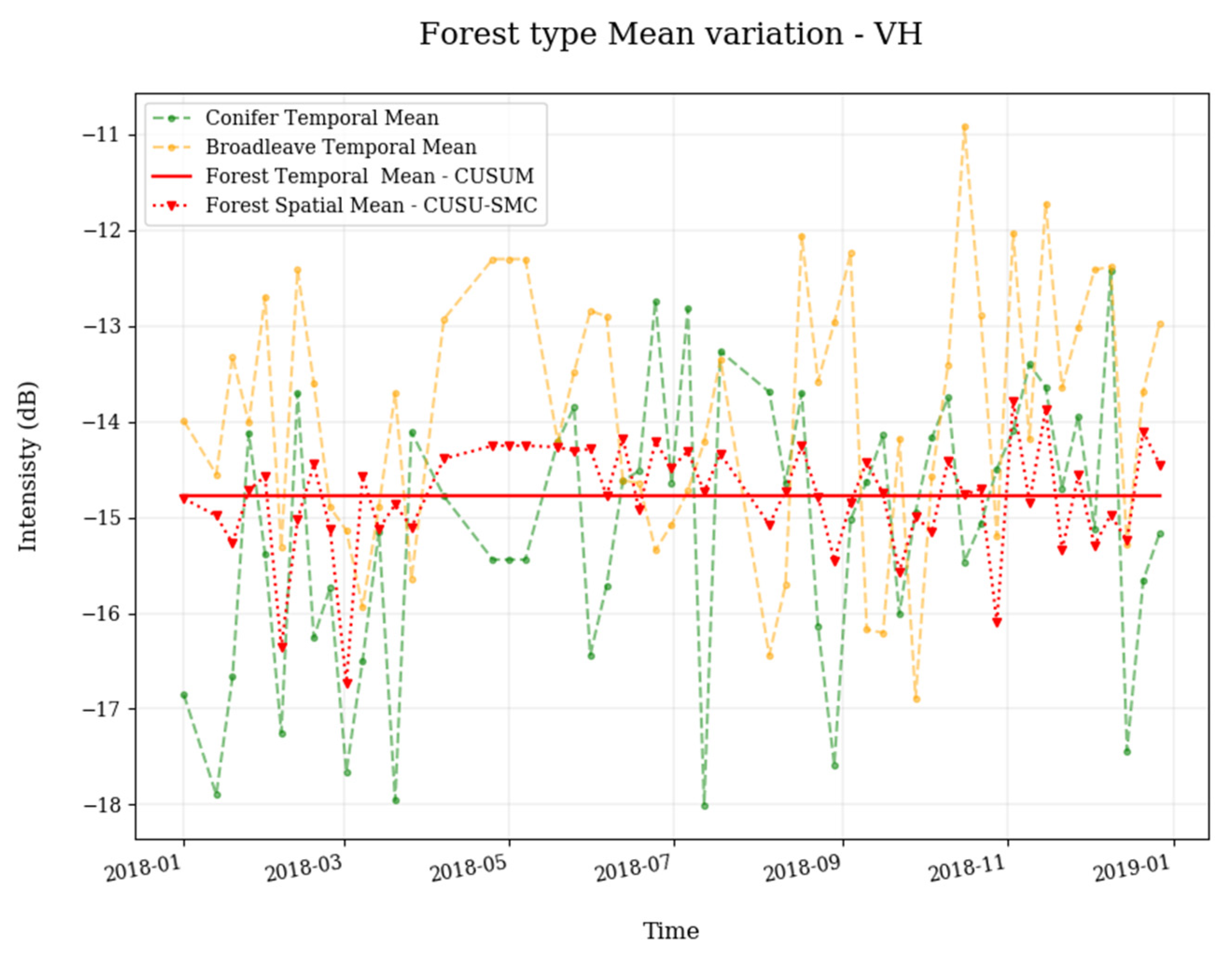
- Temporal mean|CUSUM
- (2)
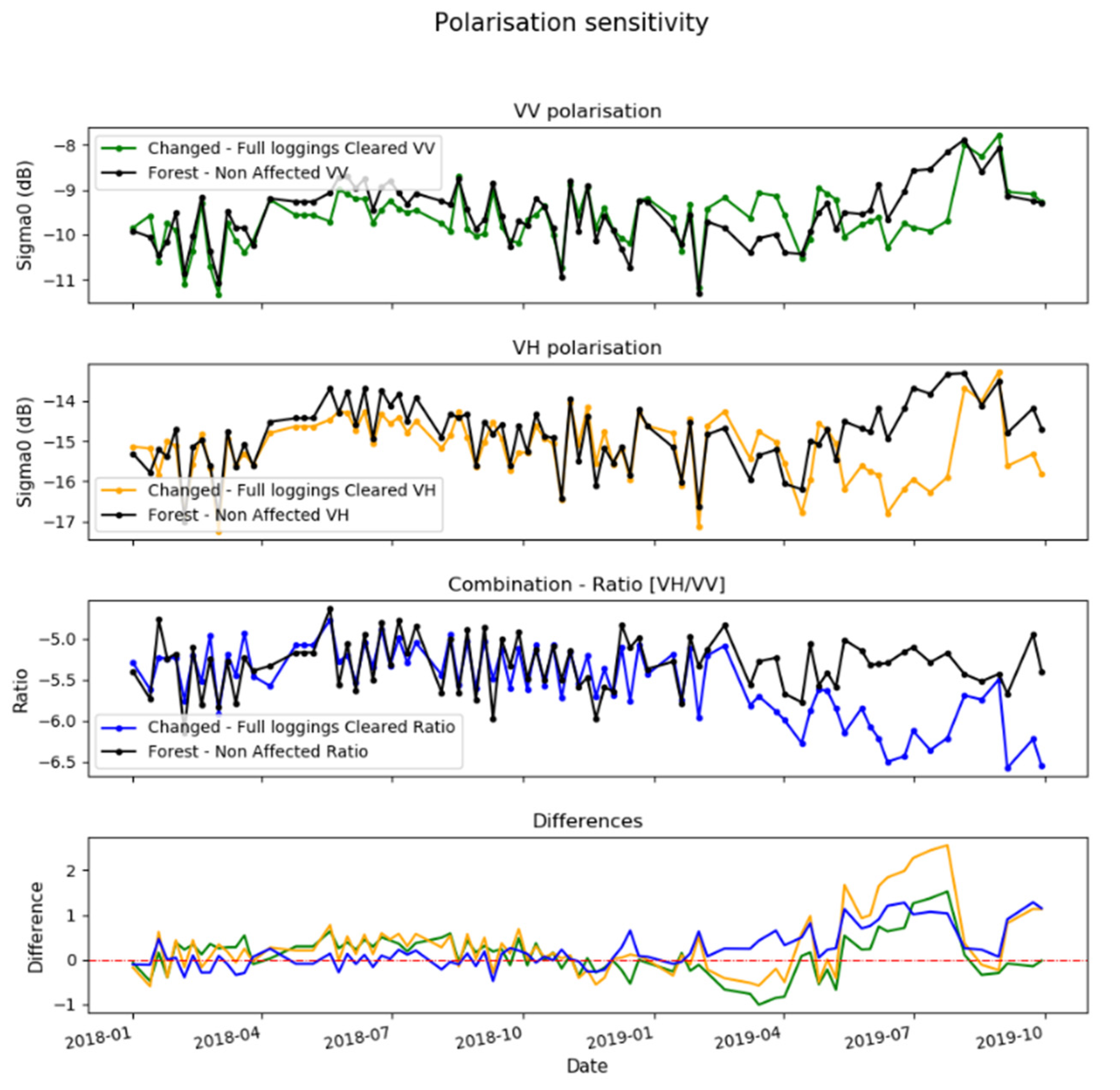
- Spatial mean|CUSU-SMCwhere = 0 and i is an iteration over the temporal axis of the cube. Nt is the total number of acquisitions used in the training dataset. The image I can be the VV, VH polarization channels or their ratio. The comparison of results using the three observables is provided in the following.
4.4. Z Score Calculation
4.5. Logging Area Detection Accuracy Assessment
4.6. Post-Processing and Sieve Filtering
4.7. CUSUMs Framework
5. Results
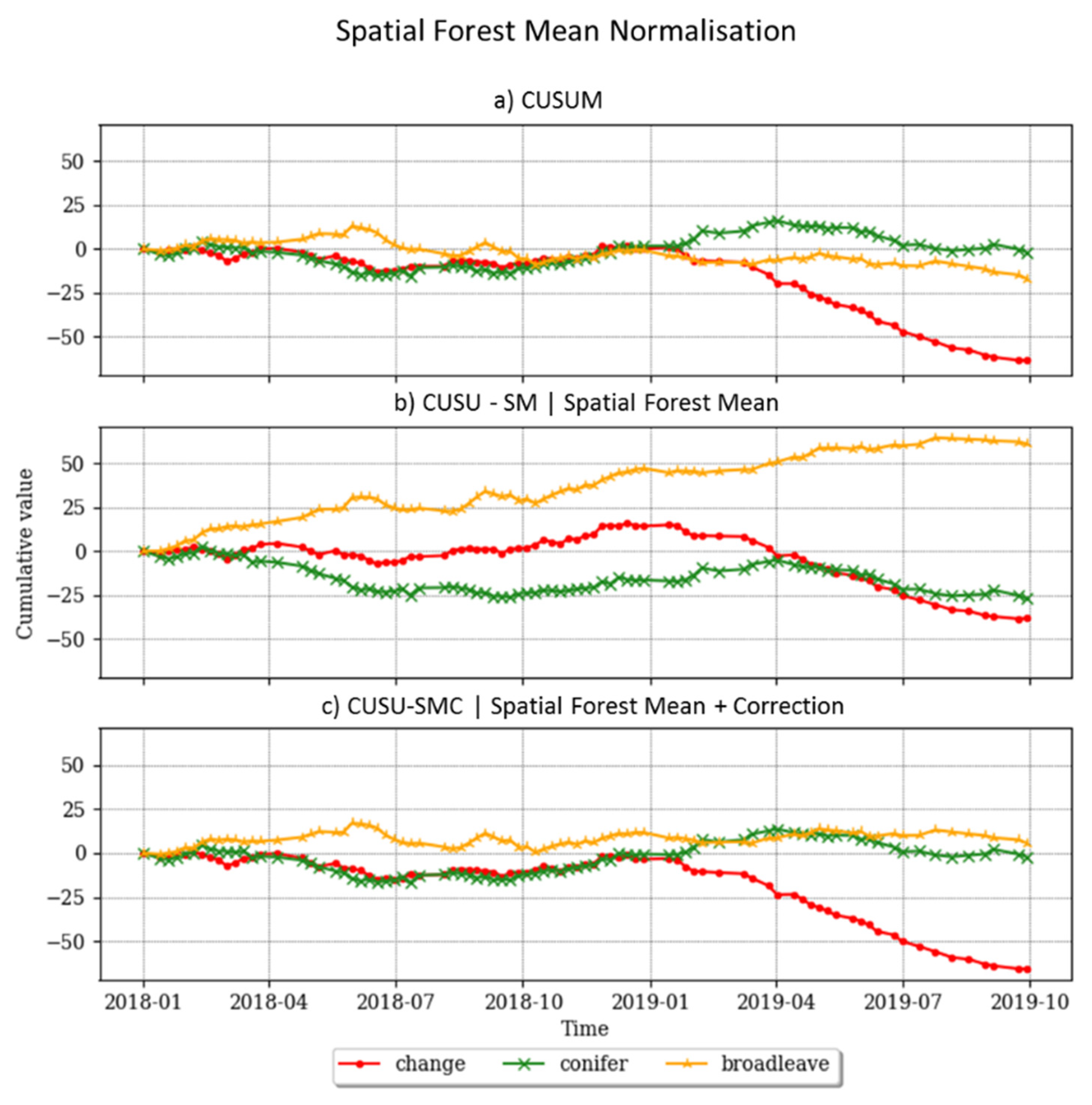
5.1. Trends and Biases of CUSUMs
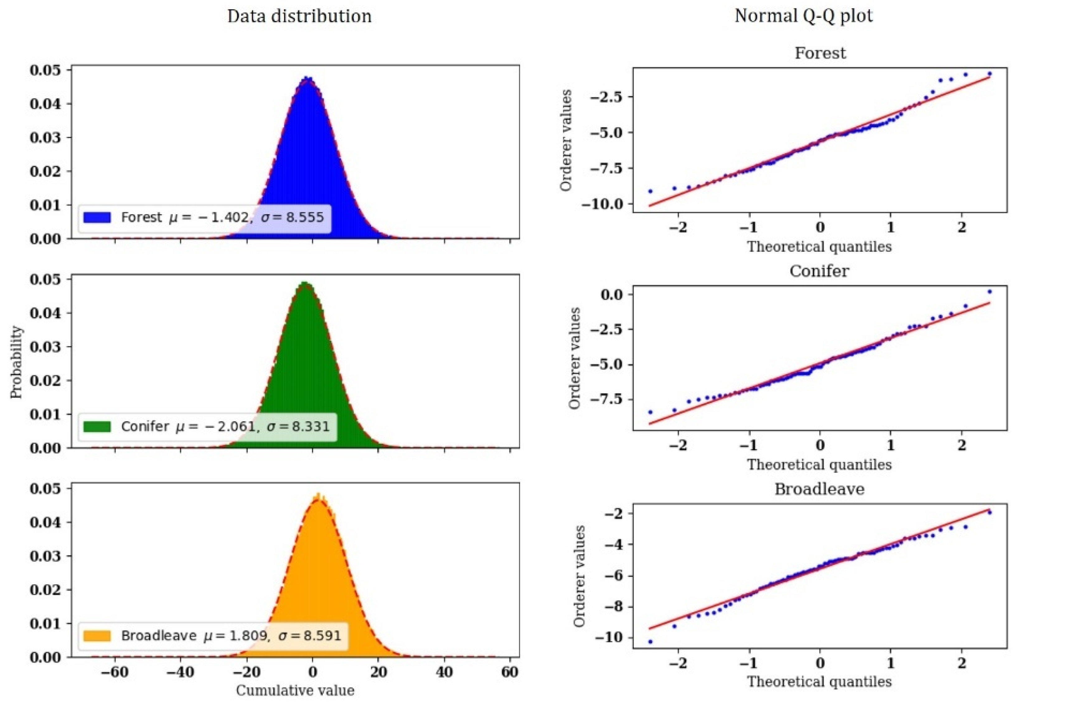
5.2. Testing the Assumptions
5.3. CUSUM Logging Activities Detection
5.3.1. Comparison with Pairwise Analysis
- Continuous pairwise. This approach aims to generate a continuous change analysis based on the comparison of each image present in the timeseries to the image acquired three times before.where, i is an iteration over the temporal axis of the cube. Nt is the total number of acquisitions used in the training dataset. The image I used for the analysis corresponds to a channel, or the ratio after applying a boxcar filter (window size = 3).
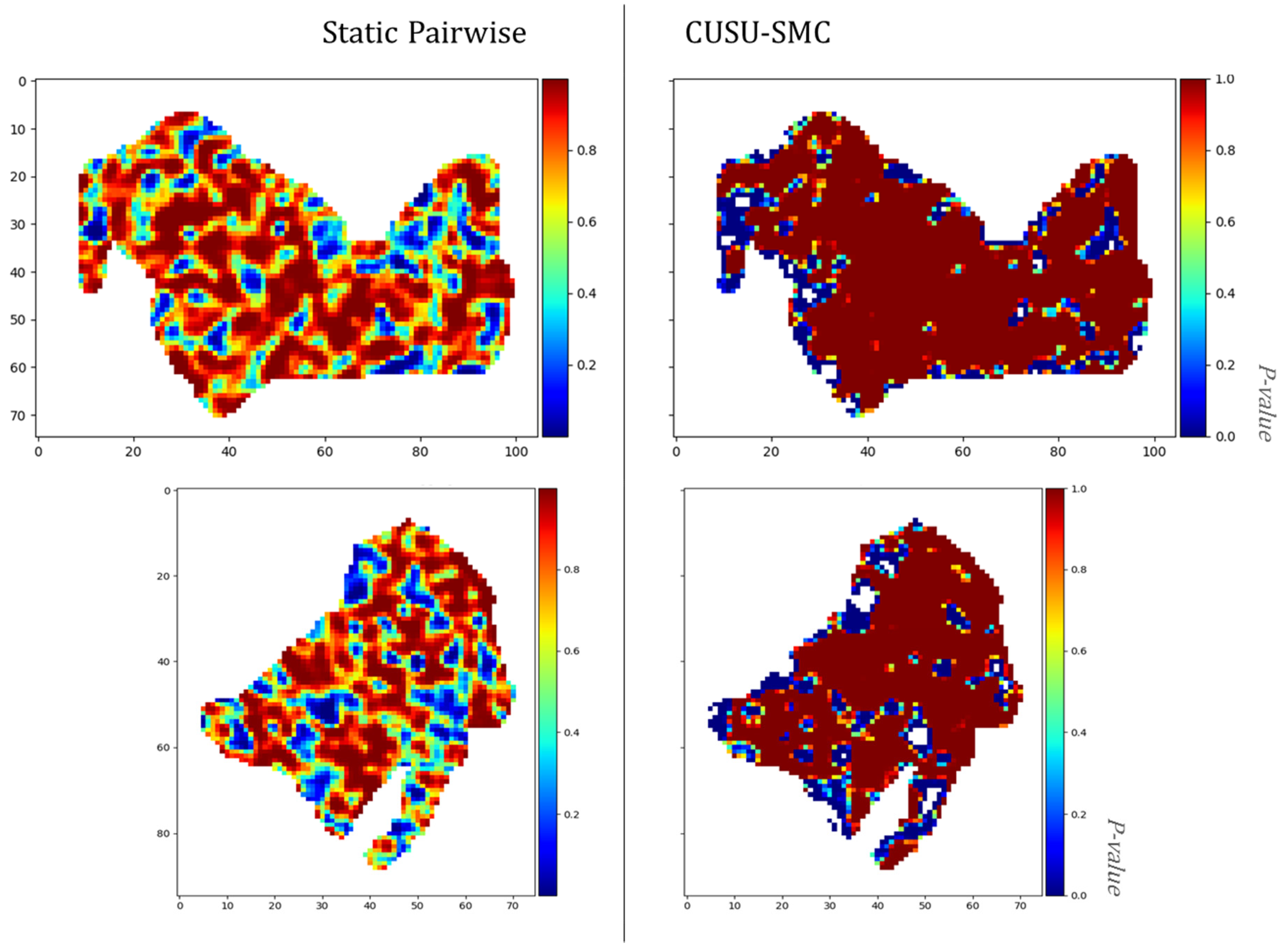
- Static pairwise. This methodology follows the common direct pairwise change detection, by which two acquisitions separated in time by a specific event (clear-cut activities in our study case) are directly compared. Considering that all logging activity studies were carried out between 1 December 2018 and 20 June 2019, we have used the image acquired on 3 November 2018 as the reference image (pre-event), and the last image of the timeseries acquired on 29 September 2019 as the change image (post-event).
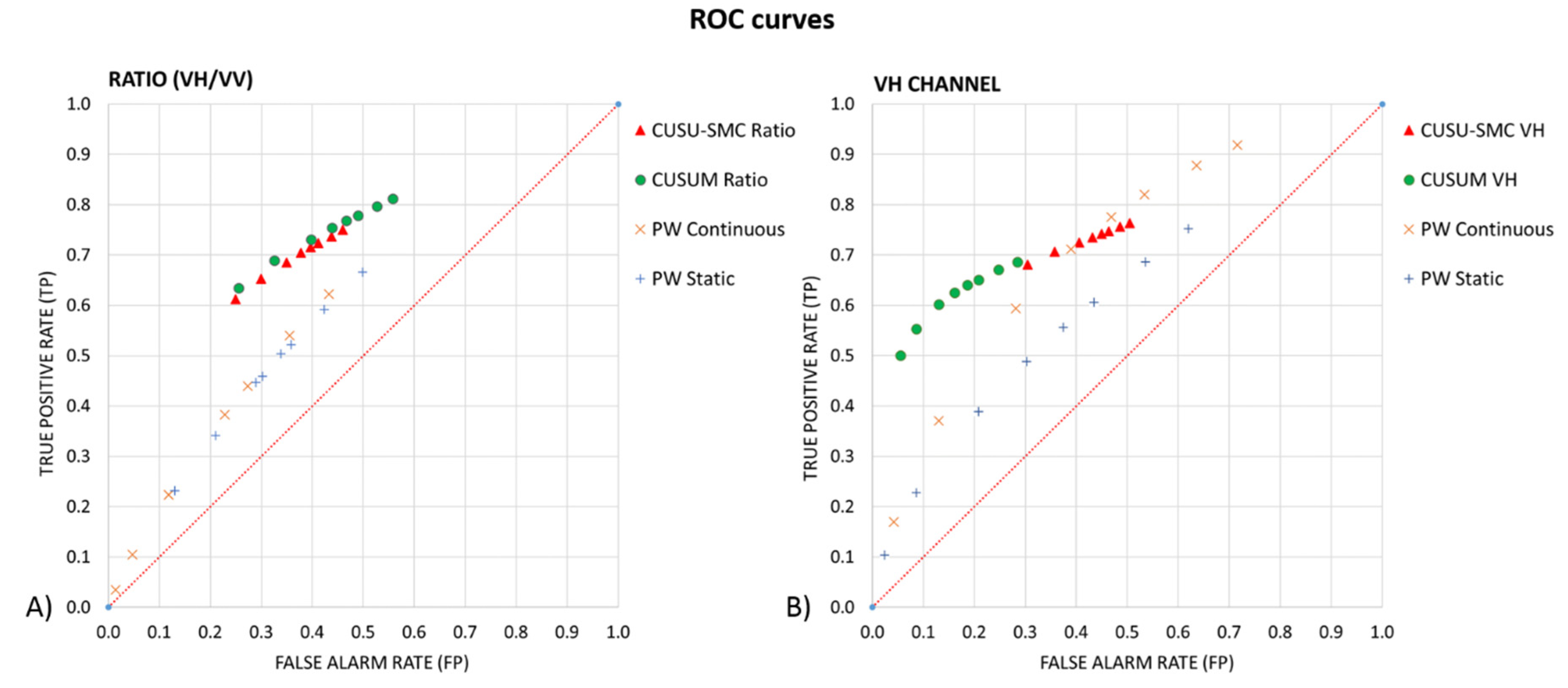
5.3.2. ROC Curves
5.3.3. Final Detection Mask
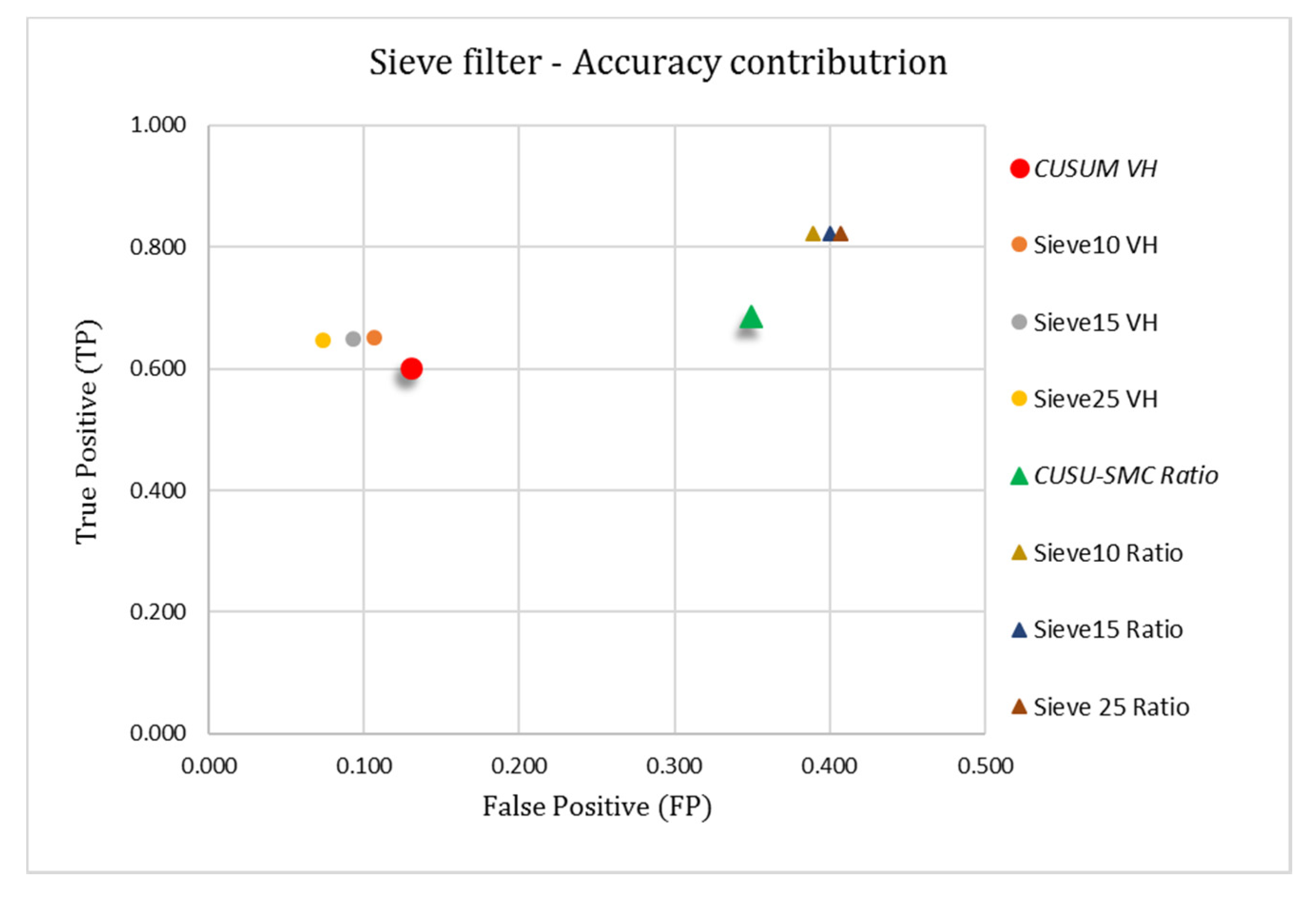
5.4. Post-Processing Sieve Filter
5.5. Forest Logging Detection Maps with Sieve Filter
6. Discussion
6.1. Near Real Time
6.2. Adaptability to Other Sensors and Applications (Synergies)
6.3. Limitations and Future Work
7. Conclusions
Author Contributions
Funding
Acknowledgments
Conflicts of Interest
References
- Nunes, L.J.R.; Meireles, C.I.R.; Gomes, C.J.P.; Ribeiro, N.M.C.A. Forest contribution to climate change mitigation: Management oriented to carbon capture and storage. Climate 2020, 8, 21. [Google Scholar] [CrossRef]
- Federici, S.; Tubiello, F.N.; Salvatore, M.; Jacobs, H.; Schmidhuber, J. New estimates of CO2 forest emissions and removals: 1990–2015. For. Ecol. Manage. 2015, 352, 89–98. [Google Scholar] [CrossRef]
- FAO Forest threats. Unasylva An Int. J. For. For. Ind. 2004, 55, 1.
- IUCN. Deforestation and Forest Degradation; International Union for Conservation of Nature: Gland, Switzerland, 2017. [Google Scholar]
- Kissinger, G.; Herold, M.; De Sy, V. Drivers of Deforestation and Forest Degradation: A Synthesis Report for REDD+ Policymakers; Lexeme Consulting: Vancouver, BC, Canada, 2012. [Google Scholar]
- FAO. UN-REDD Fact Sheet: About REDD+. Fao Undp Unep 2015, 1–4. [Google Scholar]
- Defries, R.S. Why Forest Monitoring Matters for People and the Planet. In Global Forest Monitoring from Earth Observation; Achard, F., Hansen, M., Eds.; CRC Press/Taylor & Francis: Boca Raton, FL, USA, 2013; pp. 1–14. [Google Scholar]
- Rudel, T.K. How Do People Transform. Landscapes? A Sociological Perspective on Suburban Sprawl and Tropical Deforestation 1. Am. J. Sociol. 2009, 115, 129–154. [Google Scholar] [CrossRef]
- Saxe, H.; Cannell, M.G.R.; Johnsen, Ø.; Ryan, M.G.; The, S.; Phytologist, N.; Mar, N.; Saxe, H.; Cannell, M.G.R.; Ryan, M.G.; et al. Tree and forest functioning in response to global warming. Tansley Rev. 2001, 149, 369–399. [Google Scholar] [CrossRef]
- Apps, M.J. Forests, the global carbon cycle and climate change. In Congress Proceedings, B—Forests for the Planet; XII World Forestry Congress: Quebec, QC, Canada, 2003; pp. 21–28. [Google Scholar]
- Bastin, J.-F.; Finegold, Y.; Garcia, C.; Mollicone, D.; Rezende, M.; Routh, D.; Zohner, C.M.; Crowther, T.W. The global tree restoration potential. Science 2019, 365, 76–79. [Google Scholar] [CrossRef]
- GOV. UK Forest 2020—Case Study—GOV. UK Space Agency: Swindon , UK, 2017. Available online: https://www.gov.uk/government/case-studies/ecometrica-forest-monitoring-systems (accessed on 16 September 2020).
- Plummer, S.; Lecomte, P.; Doherty, M. The ESA Climate Change Initiative (CCI): A European contribution to the generation of the Global Climate Observing System. Remote Sens. Environ. 2017, 203, 2–8. [Google Scholar] [CrossRef]
- Mitchard, E. The hectares indicators: A Review of Earth Observation Methods for Detecting and Measuring Forest Change in the Tropics; Ecometrica: Edinburgh, UK, 2016; ISBN 9780995691810. [Google Scholar]
- Chuvieco, E. Fundamentals of Satellite Remote Sensing: An Environmental Approach, 2nd.; CRC Press/Taylor & Francis: Boca Raton, FL, USA, 2016; ISBN 9781498728058. [Google Scholar]
- Rüetschi, M.; Small, D.; Waser, L.; Rüetschi, M.; Small, D.; Waser, L.T. Rapid Detection of Windthrows Using Sentinel-1 C-Band SAR Data. Remote Sens. 2019, 11, 115. [Google Scholar] [CrossRef]
- Tanase, M.A.; Villard, L.; Pitar, D.; Apostol, B.; Petrila, M.; Chivulescu, S.; Leca, S.; Borlaf-Mena, I.; Pascu, I.S.; Dobre, A.C.; et al. Synthetic aperture radar sensitivity to forest changes: A simulations-based study for the Romanian forests. Sci. Total Environ. 2019, 689, 1104–1114. [Google Scholar] [CrossRef]
- Verbyla, D.L.; Kasischke, E.S.; Hoy, E.E. Seasonal and topographic effects on estimating fire severity from Landsat TM/ETM+ data. Int. J. Wildl. Fire 2008, 17, 527–534. [Google Scholar] [CrossRef]
- Schmitt, M.; Hughes, L.H.; Zhu, X.X. The SEN1-2 dataset for deep learning in SAR-optical data fusion. In Proceedings of the ISPRS Annals Photogrammretry Remote Sense Spatial Information Sciences, Karlsruhe, Germany, 10–12 October 2018; Volume IV-1, pp. 141–146. [Google Scholar]
- Polarimetry Tutorial PolSARpro ESA. Available online: https://earth.esa.int/web/polsarpro/polarimetry-tutorial (accessed on 16 July 2019).
- Podest, E. Conceptos Básicos del Radar de Apertura Sintética 2017. Available online: https://arset.gsfc.nasa.gov/sites/default/files/water/Brazil_2017/Day1/S1P2-span.pdf (accessed on 25 July 2020).
- JJ-FAST. Available online: https://www.eorc.jaxa.jp/jjfast/jj_index.html (accessed on 20 August 2020).
- Hansen, M.C.; Potapov, P.V.; Moore, R.; Hancher, M.; Turubanova, S.A.; Tyukavina, A.; Thau, D.; Stehman, S.V.; Goetz, S.J.; Loveland, T.R.; et al. High-Resolution Global Maps of 21st-Century Forest Cover Change. New Ser. 2013, 342, 850–853. [Google Scholar] [CrossRef]
- Shimada, M.; Itoh, T.; Motooka, T.; Watanabe, M.; Shiraishi, T.; Thapa, R.; Lucas, R. New global forest/non-forest maps from ALOS PALSAR data (2007–2010). Remote Sens. Environ. 2014, 155, 13–31. [Google Scholar] [CrossRef]
- Martone, M.; Rizzoli, P.; Wecklich, C.; González, C.; Bueso-Bello, J.L.; Valdo, P.; Schulze, D.; Zink, M.; Krieger, G.; Moreira, A. The global forest/non-forest map from TanDEM-X interferometric SAR data. Remote Sens. Environ. 2018, 205, 352–373. [Google Scholar] [CrossRef]
- Hardy, A.; Ettritch, G.; Cross, D.E.; Bunting, P.; Liywalii, F.; Sakala, J.; Silumesii, A.; Singini, D.; Smith, M.; Willis, T.; et al. Automatic detection of open and vegetated water bodies using Sentinel 1 to map African malaria vector mosquito breeding habitats. Remote Sens. 2019, 11, 593. [Google Scholar] [CrossRef]
- Tanase, M.A.; Perez-Cabello, F.; de la Riva, J.; Santoro, M. TerraSAR-X Data for Burn Severity Evaluation in Mediterranean Forests on Sloped Terrain. IEEE Trans. Geosci. Remote Sens. 2010, 48, 917–929. [Google Scholar] [CrossRef]
- Joshi, N.; Mitchard, E.T.; Woo, N.; Torres, J.; Moll-Rocek, J.; Ehammer, A.; Collins, M.; Jepsen, M.R.; Fensholt, R. Mapping dynamics of deforestation and forest degradation in tropical forests using radar satellite data. Environ. Res. Lett. 2015, 10, 034014. [Google Scholar] [CrossRef]
- Tanase, M.A.; Kennedy, R.; Aponte, C. Radar Burn Ratio for fire severity estimation at canopy level: An example for temperate forests. Remote Sens. Environ. 2015, 170, 14–31. [Google Scholar] [CrossRef]
- Antropov, O.; Rauste, Y.; Väänänen, A.; Mutanen, T.; Häme, T. Mapping Forest Disturbance Usign Long Time series of Sentinel-1 data: Case studies over Boreal and Tropical Forests. In Proceedings of the 2016 IEEE International Geoscience and Remote Sensing Symposium (IGARSS), Beijing, China, 10–15 July 2016; pp. 3906–3909. [Google Scholar]
- Bouvet, A.; Mermoz, S.; Ballère, M.; Koleck, T.; Le Toan, T. Use of the SAR Shadowing Effect for Deforestation Detection with Sentinel-1 Time Series. Remote Sens. 2018, 10, 1250. [Google Scholar] [CrossRef]
- Reiche, J.; Hamunyela, E.; Verbesselt, J.; Hoekman, D.; Herold, M. Improving near-real time deforestation monitoring in tropical dry forests by combining dense Sentinel-1 time series with Landsat and ALOS-2 PALSAR-2. Remote Sens. Environ. 2018, 204, 147–161. [Google Scholar] [CrossRef]
- Tanase, M.A.; Belenguer-Plomer, M.Á.; Roteta, E.; Bastarrika, A.; Wheeler, J.; Fernández-Carrillo, Á.; Tansey, K.; Wiedemann, W.; Navratil, P.; Lohberger, S.; et al. Burned Area Detection and Mapping: Intercomparison of Sentinel-1 and Sentinel-2 Based Algorithms over Tropical Africa. Remote Sens. 2020, 12, 334. [Google Scholar] [CrossRef]
- Belenguer-Plomer, M.A.; Chuvieco, E.; Tanase, M.A. Temporal decorrelation of c-band backscatter coefficient in mediterranean burned areas. Remote Sens. 2019, 11, 2661. [Google Scholar] [CrossRef]
- Ruiz-Ramos, J.; Marino, A.; Boardman, C.P. Using sentinel 1-SAR for monitoring long term variation in burnt forest areas. In Proceedings of the International Geoscience and Remote Sensing Symposium (IGARSS), Valencia, Spain, 22–27 July 2018. [Google Scholar]
- Watanabe, M.; Koyama, C.N.; Hayashi, M.; Nagatani, I.; Shimada, M. Early-stage deforestation detection in the tropics with L-band SAR. IEEE J. Sel. Top. Appl. Earth Obs. Remote Sens. 2018, 11, 2127–2133. [Google Scholar] [CrossRef]
- Soil Survey of Scotland Staff. Soil Maps of Scotland at a Scale of 1:250 000; Soil Survey of Scotland Staff: Aberdeen, Scotland, 1981. [Google Scholar]
- Torres, R.; Snoeij, P.; Geudtner, D.; Bibby, D.; Davidson, M.; Attema, E.; Potin, P.; Rommen, B.; Floury, N.; Brown, M.; et al. GMES Sentinel-1 mission. Remote Sens. Environ. 2012, 120, 9–24. [Google Scholar] [CrossRef]
- Filipponi, F. Sentinel-1 GRD Preprocessing Workflow. Proceedings 2019, 18, 11. [Google Scholar] [CrossRef]
- Ground Range Detected Sentinel-1 SAR Technical Guide Sentinel Online. Available online: https://sentinel.esa.int/web/sentinel/technical-guides/sentinel-1-sar/products-algorithms/level-1-algorithms/ground-range-detected (accessed on 21 December 2019).
- Forest Research About the NFI Forest Research. Available online: https://www.forestresearch.gov.uk/tools-and-resources/national-forest-inventory/about-the-nfi/ (accessed on 16 December 2019).
- Earth Observing System Shortwave Infrared (SWIR) For Agriculture: Band Combination. Available online: https://eos.com/shortwave-infrared/ (accessed on 17 September 2020).
- Manogaran, G.; Lopez, D. Spatial cumulative sum algorithm with big data analytics for climate change detection R. Comput. Electr. Eng. 2017, 65, 207–221. [Google Scholar] [CrossRef]
- Kellndorfer, J. Using SAR data for Mapping Deforestation and Forest Degradation. In The SAR Handbook. Comprehensive Methodologies for Forest Monitoring and Biomass Estimation; ServirGlobal: Hunstville, AL, USA, 2019; pp. 65–79. [Google Scholar]
- Bullock, E.L.; Woodcock, C.E.; Holden, C.E. Improved change monitoring using an ensemble of time series algorithms. Remote Sens. Environ. 2020, 238, 111165. [Google Scholar] [CrossRef]
- Kucera, J.; Barbosa, P.; Strobl, P. Cumulative Sum Charts—A Novel Technique for Processing Daily Time Series of MODIS Data for Burnt Area Mapping in Portugal. In Proceedings of the 2007 International Workshop on the Analysis of Multi-Temporal Remote Sensing Images, Leuven, Belgium, 18–20 July 2007; pp. 1–6. [Google Scholar]
- NCSS, L. Cumulative Sum (CUSUM) Charts. In NCSS 2019 Statistical Software (2019); © NCSS, LLC: Kaysville, UT, USA, 2019; pp. 247-1–247-20. [Google Scholar]
- Sasaki, Y.; Fellow, R. The Truth of the F-Measure, Manchester: MIB-School of Computer Science; University of Manchester: Manchester, UK, 2007. [Google Scholar]
- Ghoneim, S. Accuracy, Recall, Precision, F-Score & Specificity, which to optimize on? Available online: https://towardsdatascience.com/accuracy-recall-precision-f-score-specificity-which-to-optimize-on-867d3f11124 (accessed on 7 June 2020).
- GDAL/OGR contributors. GDAL/OGR Geospatial Data Abstraction Software Library; Open Source Geospatial Foundation: Chicago, IL, USA, 2018. [Google Scholar]
- Ose, K. Detection and Mapping of Clear-Cuts with Optical Satellite Images. In QGIS and Applications in Agriculture and Forest; John Wiley & Sons, Inc.: Hoboken, NJ, USA, 2018; pp. 153–180. ISBN 9781119457107. [Google Scholar]
- Green, R.M. The sensitivity of SAR backscatter to forest windthrow gaps. Int. J. Remote Sens. 1998, 19, 2419–2425. [Google Scholar] [CrossRef]
- Eriksson, L.E.B.; Fransson, J.E.S.; Soja, M.J.; Santoro, M. Backscatter signatures of wind-thrown forest in satellite SAR images. In Proceedings of the 2012 IEEE International Geoscience and Remote Sensing Symposium, Munich, Germany, 22–27 July 2012; pp. 6435–6438. [Google Scholar]
- Tanase, M.A.; Aponte, C.; Mermoz, S.; Bouvet, A.; Le, T.; Heurich, M. Remote Sensing of Environment Detection of windthrows and insect outbreaks by L-band SAR: A case study in the Bavarian Forest National Park. Remote Sens. Environ. 2018, 209, 700–711. [Google Scholar] [CrossRef]
- Quegan, S.; Le Toan, T.; Yu, J.J.; Ribbes, F.; Floury, N. Multitemporal ERS SAR analysis applied to forest mapping. IEEE Trans. Geosci. Remote Sens. 2000, 38, 741–753. [Google Scholar] [CrossRef]
- Ulehla, Z.J.; Martin, R.F. Operating characteristic analysis of attribute ratings. Behav. Res. Methods Instrum. 1971, 3, 291–293. [Google Scholar] [CrossRef]
- Zhuang, H.; Fan, H.; Deng, K.; Yu, Y. An improved neighborhood-based ratio approach for change detection in SAR images. Eur. J. Remote Sens. 2018, 51, 723–738. [Google Scholar] [CrossRef]
- Zweig, M.H.; Campbell, G. Receiver-Operating Characteristic (ROC) Plots: A Fundamental Evaluation Tool in Clinical Medicine. Clin. Chem. 1993, 39, 561–577. [Google Scholar] [CrossRef]
- Schwarz, M.; Steinmeier, C.; Holecz, F.; Stebler, O.; Wagner, H. Detection of Windthrow in Mountainous Regions with Different Remote Sensing Data and Classification Methods. Scand. J. For. Res. 2003, 18, 525–536. [Google Scholar] [CrossRef]
- Hansen, M.C.; Krylov, A.; Tyukavina, A.; Potapov, P.V.; Turubanova, S.; Zutta, B.; Ifo, S.; Margono, B.; Stolle, F.; Moore, R. Humid tropical forest disturbance alerts using Landsat data. Environ. Res. Lett. 2016, 11, 034008. [Google Scholar] [CrossRef]
- Dabboor, M.; Iris, S.; Singhroy, V. The RADARSAT Constellation Mission in Support of Environmental Applications. Proceedings 2018, 2, 323. [Google Scholar] [CrossRef]
- Canadian Space Agency (CSA) Technical characteristics-Canada.ca. Available online: https://www.asc-csa.gc.ca/eng/satellites/radarsat/technical-features/characteristics.asp (accessed on 2 March 2020).
- Montgomery, D.C.; Jennings, C.L.; Kulahci, M. Introduction to Time Series Analysis and Forecasting, 2nd ed.; John Wiley & Sons, Ed.; Wiley-Blackwell: Hoboken, NJ, USA, 2016; Volume 37. [Google Scholar]
- Stankevich, S.A.; Kozlova, A.A.; Piestova, I.O.; Lubskyi, M.S. Leaf area index estimation of forest using sentinel-1 C-band SAR data. In Proceedings of the MRRS 2017 IEEE Microwaves, Radar and Remote Sensing Symposium, Cherkasy Oblast, Ukraine, 29–31 August 2017; Institute of Electrical and Electronics Engineers Inc.: Piscataway, NJ, USA, 2017; pp. 253–256. [Google Scholar]
- Koyama, C.N.; Watanabe, M.; Hayashi, M.; Ogawa, T.; Shimada, M. Mapping the spatial-temporal variability of tropical forests by ALOS-2 L-band SAR big data analysis. Remote Sens. Environ. 2019, 233, 111372. [Google Scholar] [CrossRef]


| Product | ||
|---|---|---|
| Reference | H0 | H1 |
| H0 | True Negative (TN) | False Positive (FP) |
| H1 | False Negative (FN) | True Positive (TP) |
| CUSUM | CUSU-SMC | |||||
|---|---|---|---|---|---|---|
| VV | VH *C | Ratio (VH/VV) | VH *T | Ratio (VH/VV) | Ratio (VH/VV) *NC | |
| TP | 0.324 | 0.602 | 0.731 | 0.724 | 0.685 | 0.654 |
| TN | 0.917 | 0.870 | 0.602 | 0.594 | 0.650 | 0.583 |
| FP | 0.083 | 0.130 | 0.398 | 0.406 | 0.350 | 0.417 |
| FN | 0.676 | 0.398 | 0.269 | 0.276 | 0.315 | 0.346 |
| OA | 0.621 | 0.736 | 0.667 | 0.659 | 0.668 | 0.618 |
| PA | 0.324 | 0.602 | 0.731 | 0.724 | 0.685 | 0.654 |
| UA | 0.797 | 0.822 | 0.648 | 0.641 | 0.662 | 0.610 |
| F-score | 0.460 | 0.695 | 0.687 | 0.680 | 0.674 | 0.631 |
| CUSUMs | Pairwise | |||||
|---|---|---|---|---|---|---|
| Continuous | Static | |||||
| CUSUM *C(VH) | CUSU-SMC *T(Ratio) | Continuous Ratio | Continuous VH | Static Ratio | Static VH | |
| TP | 0.602 | 0.685 | 0.223 | 0.594 | 0.459 | 0.389 |
| TN | 0.870 | 0.650 | 0.882 | 0.718 | 0.697 | 0.792 |
| FP | 0.130 | 0.350 | 0.118 | 0.282 | 0.303 | 0.208 |
| FN | 0.398 | 0.315 | 0.777 | 0.406 | 0.541 | 0.611 |
| OA | 0.736 | 0.668 | 0.553 | 0.656 | 0.578 | 0.590 |
| PA | 0.602 | 0.685 | 0.223 | 0.594 | 0.459 | 0.389 |
| UA | 0.822 | 0.662 | 0.655 | 0.678 | 0.602 | 0.651 |
| F-score | 0.695 | 0.674 | 0.333 | 0.633 | 0.521 | 0.487 |
| OA | PA | UA | F-Score | Spatial Loss | |
|---|---|---|---|---|---|
| CUSU-SMC (Ratio) | 0.668 | 0.685 | 0.662 | 0.674 | - |
| Sieve (10 pixels) | 0.717 | 0.822 | 0.679 | 0.744 | 0.4 ha |
| Sieve (15 pixels) | 0.711 | 0.822 | 0.672 | 0.740 | 0.6 ha |
| Sieve (25 pixels) | 0.708 | 0.823 | 0.669 | 0.738 | 1 ha |
| CUSUM (VH) | 0.736 | 0.602 | 0.822 | 0.695 | - |
| Sieve (10 pixels) | 0.772 | 0.650 | 0.859 | 0.740 | 0.4 ha |
| Sieve (15 pixels) | 0.778 | 0.649 | 0.875 | 0.745 | 0.6 ha |
| Sieve (25 pixels) | 0.786 | 0.646 | 0.898 | 0.751 | 1 ha |
© 2020 by the authors. Licensee MDPI, Basel, Switzerland. This article is an open access article distributed under the terms and conditions of the Creative Commons Attribution (CC BY) license (http://creativecommons.org/licenses/by/4.0/).
Share and Cite
Ruiz-Ramos, J.; Marino, A.; Boardman, C.; Suarez, J. Continuous Forest Monitoring Using Cumulative Sums of Sentinel-1 Timeseries. Remote Sens. 2020, 12, 3061. https://doi.org/10.3390/rs12183061
Ruiz-Ramos J, Marino A, Boardman C, Suarez J. Continuous Forest Monitoring Using Cumulative Sums of Sentinel-1 Timeseries. Remote Sensing. 2020; 12(18):3061. https://doi.org/10.3390/rs12183061
Chicago/Turabian StyleRuiz-Ramos, Javier, Armando Marino, Carl Boardman, and Juan Suarez. 2020. "Continuous Forest Monitoring Using Cumulative Sums of Sentinel-1 Timeseries" Remote Sensing 12, no. 18: 3061. https://doi.org/10.3390/rs12183061
APA StyleRuiz-Ramos, J., Marino, A., Boardman, C., & Suarez, J. (2020). Continuous Forest Monitoring Using Cumulative Sums of Sentinel-1 Timeseries. Remote Sensing, 12(18), 3061. https://doi.org/10.3390/rs12183061