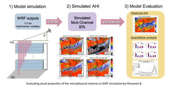
Satellite Observation for Evaluating Cloud Properties of the Microphysical Schemes in Weather Research and Forecasting Simulation: A Case Study of the Mei-Yu Front Precipitation System

Abstract

Radiative transfer model can be used to convert the geophysical variables (e.g., atmospheric thermodynamic state) to the radiation field. In this study, the Community Radiative Transfer Model (CRTM) is used to connect regional Weather Research and Forecasting (WRF) model outputs and satellite observations. A heavy rainfall event caused by the Mei-Yu front on the June 1, 2017, in the vicinity of Taiwan, was chosen as a case study. The simulated cloud performance of WRF with four microphysics schemes (i.e., Goddard (GCE), WRF single-moment 6 class (WSM), WRF double-moment 6 class (WDM), and Morrison (MOR) schemes) was investigated objectively using multichannel observed satellite radiances from a Japanese geostationary satellite Himawari-8. The results over the East Asia domain (9 km) illustrate that all four microphysics schemes overestimate cloudy pixels, in particular, the high cloud of simulation with MOR when comparing with satellite data. Sensitivity tests reveal that the excess condensation of ice at ≥14 km with MOR might be associated with the overestimated high cloud cover. However, GCE displayed an improved performance on water vapor channel in clear skies. When focusing on Taiwan using a higher (3 km) model resolution, each scheme displayed a decent performance on cloudy pixels. In the grid-by-grid skill score analysis, the distribution of high clouds was the most accurate among the three cloud types. The results also suggested that all schemes required a longer simulation time to describe the low cloud horizontal extend.

1. Introduction

Clouds play a crucial role in the Earth system. For instance, cloud coverage can affect the temperature [1,2] and global radiation balance [3,4]. In the global model, clouds are a crucial element of the Earth system because of their interaction with the longwave and shortwave radiation of the Earth and Sun. Furthermore, cloud coverage and cloud properties have substantial implications on forecasting convection initiation [5,6] and severe weather [7] at the regional level. Therefore, evaluating radiation is vital in numerical models.

The observed rain is a typical parameter to evaluate numerical weather prediction (NWP) model performance. However, the precipitation is initiated by the condensation of water vapor, followed by a sophisticated cloud-to-precipitation process. Therefore, obtaining information regarding cloud formation within NWP model simulation is an essential step for the evaluation of the model performance, because the NWP model combines the macrophysical and microphysical processes of the atmosphere and clouds [8,9,10]. In the numerical model, microphysics parameterization schemes are used to describe the nucleation of cloud droplets from water vapor to different hydrometeors explicitly. However, each parametrization method may have slightly different assumptions and provide different coefficients in the microphysics schemes, and thus the selection of the parametrization schemes will affect the results of model simulations [11,12,13,14]. Therefore, the validation and evaluation of different parameterization schemes in the numerical weather model are essential.

Conventionally, the performance of a numerical model is evaluated by comparison with available observations, such as surface observations, sounding data, or other kinematic or thermodynamic fields. However, the in situ observations of the convective systems, such as atmospheric profiles from radiosondes or direct measurements from aircraft penetrating cumulus clouds, have insufficient temporal and spatial distribution, which hinders comprehensive validation of the performance of the models. Advances in meteorological satellite technology have collected consistent and high spatiotemporal resolution remote sensing data using satellites. Therefore, the simulation performance of the model can be evaluated comprehensively by using meteorological satellite data. However, the satellite sensor measures reflectance and radiance of the visible and infrared bands, respectively. Both represent the reflected and emitted radiation from a particular area and azimuth angle, within a specific wavelength range. The radiative quantities cannot be directly compared with the geophysical variables produced by the NWP model because of unmatched natural properties.

To evaluate the performance of the NWP model output with satellite observations, two typical methods are commonly adopted. One of the evaluation methods uses satellite observed reflectance and radiances to retrieve geophysical variables, such as atmospheric moisture, temperature, cloud characteristics, and surface information. Previous studies have used retrieval data to analyze the performance of numerical models of atmospheric water vapor, cloud properties, precipitation, and atmospheric thermodynamic state, among others [15,16,17,18]. However, the retrieval technique may solve an ill-posed problem, which consumes more computational resources, and may cause uncertainty in the retrieved products. The second method uses a radiative transfer model to perform forward calculation to convert the geophysical variables from model outputs to simulated observations by satellite, also known as “model-to-satellite evaluation” [19,20,21,22,23,24,25,26]. This method has the benefit of using fewer computational resources and avoids the uncertainties caused by ill-posed conditions in the retrieval algorithm. As the radiometry observations are sensitive to the cloud properties, profiles of the atmospheric and surface features, “model-to-satellite evaluation” method, is an economic and efficient tool for evaluating the NWP model in studies on cloud formation, microphysical properties, and interactions with precipitation [27,28,29,30].

Studies on the characteristics of the microphysical parameterization schemes have typically compared with ground-based radar or polar-orbiting satellite (e.g., TRMM) observation to obtain the information on rainfall because of the low resolution of geostationary satellites [31,32,33]. Advances in satellites have enabled higher spatial, temporal, and radiometric resolution observational data. Therefore, high grid resolution NWP model simulations can more readily be evaluated against satellite observations. For example, Grasso et al. [34] used simulated satellite images to evaluate the performance of the Regional Atmospheric Modeling System (RAMS model) and identified coding errors in microphysical routines. Jankov et al. [35] conducted a simulation with five different microphysics schemes for the atmospheric river event and evaluated the influence on radiance for different microphysics schemes. Liu et al. [36] used the simulated satellite observations to evaluate the performance of the cloud distribution of each cloud type from Taiwan’s Central Weather Bureau global forecast system using two different cumulus schemes with MTSAT-2 and identified characteristics of these cumulus schemes. Yao et al. [37] used FY-2E to evaluate the performance of the cloud in Weather Research and Forecasting (WRF) using a single microphysical scheme, and they illustrated the characteristics of different cloud types over mainland China.

To evaluate regional NWP model simulation for high-impact weather, the observation of ground-based radar reflectivity or rain gauge was commonly adopted. However, the results reflect the later stage or the final results but not the former stage of the precipitation event, which may cause a “correct answer because of wrong reason” situation. A rainfall event must go through all the stages, such as convection initiation and the formation of clouds. However, the model simulation does not necessarily capture the cloud structures. The uncertainty that occurs before the onset of precipitation has been investigated by Chung et al. [38]. Model evaluations of clouds should not neglect this factor.

The main goal of this study was to evaluate the radiance performance of an NWP model in the East Asian region using multichannel satellite images. A typical frontal system, namely Mei-Yu, was selected for our case study. The results were compared with geosynchronous satellites with high spatial and temporal resolution. The simulated Himawari-8 satellite imagery was produced using the simulation output from the WRF model coupled with the Community Radiative Transfer Model (CRTM) forward model. As the simulation of clouds was affected by the choice of the microphysics schemes in WRF, comparing the brightness temperature (BT) using various microphysics schemes may provide additional information (e.g., the cloud distribution, and cloud top height, etc.) regarding the characteristics of these microphysics schemes.

The remainder of this paper is organized as follows: Section 2 describes the precipitation event selected, the NWP model used, and the observed satellite. Section 3 introduces the radiative transfer model CRTM, the cloud classification method, and the verification methods. Section 4 presents the results, including the performance of clouds over East Asia with coarser resolution simulation, the analysis of cloud pattern for the frontal system near Taiwan with higher resolution simulation, and the moisture information on the clear pixels. Finally, Section 5 summarizes the findings of the present stage and presents future works.

2. Case Description, Model Setup, and Data Source

2.1. Selected Mei-Yu Case

The Mei-Yu front event, which was accompanied by heavy rainfall on June 1–4, 2017, over Taiwan, was selected in this study. This frontal system began to affect Taiwan with southwestern airflow which brought precipitation to the mountainous regions of Central and Southern Taiwan on June 1 (local time). The front then approached the offshore of northern Taiwan in the early hours of June 2. Notably, the position of the frontal system remained in the north of Taiwan, delaying the actual rainfall time by approximately 6 h from the forecast time. A maximum hourly rainfall of >80 mm was observed at several stations in northern Taiwan. The 4-day (June 1–4) accumulated rainfall in the central and southern mountains exceeded 1000 mm in several places and caused floods, agricultural damage, and economic losses. Studies have analyzed this case and obtained results; for instance, Tu et al. [39] determined that a marine boundary layer jet that caused moisture transport was a crucial factor in this heavy rainfall case. Lupo et al. [40] investigated the sensitivity of WRF ensemble forecasts to the tuning configuration and implementation of Stochastic perturbed parameterization tendencies (SPPT) and individual independent SPPT (iSPPT) schemes with a heavy rainfall event.

2.2. Evolution of Convection and Precipitation

The structure of front moving toward Taiwan in the Mei-Yu season may change and decelerate because of enhanced ascending motion close to the terrain [41,42]. Furthermore, the southwest monsoon often forms a strong wind area near Taiwan because of the terrain effects and subtropical high [39,43], and the atmospheric conditions during the Mei-Yu season are often advantageous for the development of convection. Therefore, various mesoscale weather phenomena often accompany the transit of the Mei-Yu front in Taiwan. For instance, the frontal system often accompanies a mesoscale convective system (MCS).

Infrared satellite images can reveal the structure of the front and are used to track the MCS [43,44]. The satellite images during this Mei-Yu event revealed that the front is a complex system, composed of several convection systems (e.g., Chimney cloud with convective hot spots). Observation of metrological radars (Figure 1) indicated that the rain band of the frontal system moved toward northern Taiwan on June 1 at 1800 universal time coordinated (UTC) and then slowed and stagnated for approximately 6 h. The stratiform rainfall area was parallel to the squall line, similar to a parallel-stratiform type convection system [45].

The disaster report from Taiwan’s National Science and Technology Center for Disaster Reduction (NCDR) reported the daily accumulated rainfall from June 1 to 4 local solar time (LST) (May 31 at 1600 UTC to June 3 at 1600 UTC). Before June 1, the rainfall was mainly located in the south-central mountainous region because of the southwesterly moist flow. On June 2, the front stagnated in northern Taiwan before noon, causing intense rainfall at Keelung and the north coast area. The rainfall area gradually moved southward on June 3 and then remained in the central area. Finally, the rain began weakening on June 4.

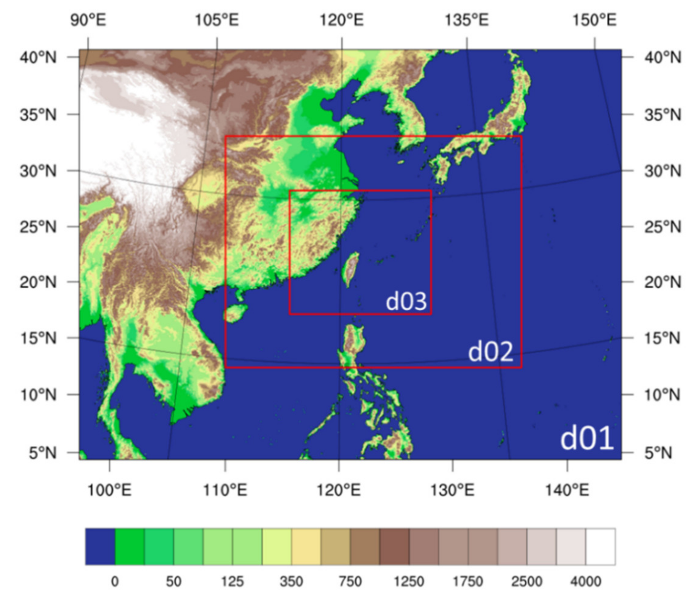
2.3. WRF Model Configurations

The nonhydrostatic WRF model (version 3.9) was used in this study. The simulation was initialized on June 1, 2017 at 1200 UTC. Three nested domains were applied over East Asia for the configuration (Figure 2). The model comprised a total of 52 vertical layers from the surface to 10 hPa, and the horizontal grid resolutions were 27, 9, and 3 km, respectively. The European Centre for Medium-Range Weather Forecasts ERA-Interim (0.75° × 0.75°) analysis was used as the initial conditions and boundary conditions.

The physical parameterizations used in this study contained the Rapid Radiative Transfer Model for broadband longwave radiation schemes [46], the Dudhia shortwave scheme [47], the Yonsei University (YSU) planetary boundary layer scheme [48], and the Kain–Fritsch cumulus parameterization [49]. The cumulus scheme was only switched on in domains 1 and 2. Microphysics schemes, which are the main focus for evaluation purposes, were performed by selecting Goddard (GCE; Tao et al. [50]), WRF single-moment in 6-class (WSM; Hong et al. [51]), WRF double-moment in 6-class (WDM; Lim et al. [52]), and Morrison (MOR; Morrison et al. [53]) schemes. Each model was integrated for 24 h with a time step of 90, 30, and 10 s in domains 1, 2, and 3, respectively.

2.4. BT from Satellite Observation

The Japanese Himawari-8 satellite data was used as a reference to evaluate the performance of the model simulation. Himawari-8 is a new-generation geostationary meteorological satellite that was launched on October 7, 2014 at 0516 UTC and reached its operational orbit in October 2014, at 35,786 km and 140.7° E with 16 bands that cover the wavelengths from visible to IR. The spatial resolution at nadir was 0.5 or 1 km for visible and near-infrared bands and 2 km for infrared bands [54]. The onboard Advanced Himawari Imager (AHI) enabled the performance of a full disk scan within a 10-min interval. Compared with the previous generation of geostationary meteorological satellites (e.g., Himawari-7, so called MTSAT-2), the onboard AHI had the advantages of enhanced observation capabilities. The number of observation bands increased from 5 to 16 [55], and the spatial and temporal resolutions improved significantly. Furthermore, the increased observation samples and denser data update rate provided more information on the atmosphere.

In this study, four channels were used to evaluate the cloud features from the model simulations. These four channels were the atmospheric window channel (10.4 µm) along with three water vapor channels (6.2, 6.9, and 7.3 µm). These four channels have several applications; for instance, the window channel can represent surface or cloud-top temperature and water vapor channels are associated with the moisture information at different altitudes. (

Table 1. Characteristics of the four Himawari-8 infrared channels used in the present study.

Channel	Central λ (μm)	Application
Window channel	10.4	Surface or cloud-top temperature
Water vapor channel	6.2, 6.9, 7.3	Mid-to-high-level water vapor

).

3. Methodology

3.1. CRTM

With the atmospheric thermodynamic and dynamic states that are simulated by the NWP model, we can use a radiative transfer model as an observation operator that considers the emission, scattering, and absorption process of radiation in the atmosphere, to obtain a proxy of the radiance observed by satellite. In this study, the information on the cloud and atmospheric conditions produced by WRF were coupled with a forward calculation model, the CRTM, to compute the simulated infrared (IR) BT as the observation using an AHI onboard the Himawari-8.

The CRTM was developed at the Joint Center for Satellite Data Assimilation, which is a multiagency research center to improve the use of satellite data for analyzing and predicting the weather, the ocean, the climate, and the environment in the United States, to simulate radiances for a given sensor from the input of meteorological variables under all atmospheric and surface conditions [56].

The temperature, pressure, water vapor, surface type, altitude given by the WRF are directly inputting to CRTM to calculate the IR BTs and obtain the corresponding radiance from the top of the atmosphere. However, the WRF provides the cloud properties with the mixing ratio of each hydrometeor (e.g., mixing ratio of cloud, ice, rain, graupel, and snow), which cannot be used directly for CRTM. In CRTM, the effective radius and water path can be used to determine the optical properties for each layer.

Martin et al. [57] suggested that a suitable parameterization for effective radius is formulated as:

$$R_{eff}=\frac{\Gamma \left(\mu +4\right)}{2\lambda \Gamma \left(\mu +3\right)}$$

(1)

$${\lambda }_x={\left[\frac{\pi {\rho }_x{N}_{0x}\Gamma \left({\mu }_x+4\right)}{6{\rho }_a{q}_x\Gamma \left({\mu }_x+1\right)}\right]}^{\frac{1}{4}}$$

(2)

where $q_x,$ ${\mu }_x$, and $N_{ox}$, respectively, represent the mixing ratio, shape factor, and intercept parameter; of each hydrometeor and ${\rho }_a$ is the density of air. The density of each hydrometeor (${\rho }_x$) is given follow the setting of different MP scheme. Since $N_{0x}=N_x{\lambda }_x$, the number concentration simulated by the double scheme can be considered in the calculation.

For MOR, the effective radius of ice follows the method in the source code of WRF version 3.9.1. For WSM, WDM, and GCE, the effective radius of cloud ice particles is obtained by the relationship between ice crystal mass and ice crystal radius, following the method used by Hong et al. [58]. In this study, the formulation of cloud ice effective radius follows Yao et al. [37]:

$$N_i=\underset{}{\min }\left(\underset{}{\max }\left(c{\left({\rho }_a\times \underset{}{\max }\left(q_i, {10}^{-15}\right)\right)}^d,{10}^3\right),{10}^6\right)$$

(3)

$$M_i=\frac{{\rho }_a{q}_i}{N_i}$$

(4)

$$R_i=\underset{}{\min }\left(11.9\times 0.75\times 0.163\times M_i{}^{\frac{1}{2}} , 500\times {10}^{-6}\right)$$

(5)

where c = 5.38 × 10⁷ and d = 0.75 are constants and $M_i$ is the ice crystal mass. qi, the mixing ratio of ice cloud, is given by WRF.

Before using the CRTM, users must convert the meteorological fields at levels to the layers. Layer temperatures (pressure) were calculated as an average of two levels of temperatures (pressure). The layer water path for each hydrometeor was calculated as the layer water content multiplied by the air density multiplied by the thickness of the layer. The variables used in the CRTM are listed in

Table 2. The variables used in the CRTM.

The Variables use in CRTM
Pressure (hPa) (Layer)	Pressure (hPa) (Level)
Temperature (K) (Layer)	Surface temperature (K)
Water vapor mixing ratio (kg/kg) (Layer)	Cloud effective radius (μm) (Layer)
Cloud water path (kg/m2) (Layer)	Ice effective radius (μm) (Layer)
Ice water path (kg/m2) (Layer)	Rain effective radius (μm) (Layer)
Rain water path (kg/m2) (Layer)	Snow effective radius (μm) (Layer)
Snow water path (kg/m2) (Layer)	Graupel effective radius (μm) (Layer)
Graupel water path (kg/m2) (Layer)	Hail effective radius (μm) (Layer)
Hail water path (kg/m2) (Layer)	Satellite Zenith Angle for model
O3 (ppmv) (Layer)	Satellite Azimuth Angle for model
Surface Type	Satellite Scan Angle for model
Topography	Number of levels
Land_sea_mask	Number of indexes

.

3.2. Match of the Horizontal Resolution

As mentioned above, the spatial resolution of Himaari-8 at nadir was 2 km for infrared bands and the horizontal resolution of simulated BTs was the same as WRF model configuration. The difference in the horizontal resolution should be considered. When comparing the simulated and observed BTs in domain 2 (9-km resolution), the mean of observation points in the model grid was used as the reference. On the other hand, for the comparison in domain 3 (3-km resolution), since the horizontal resolution is close to the observation, the nearest neighbor interpolation was introduced to get the observed BTs on the model grid.

3.3. The Classification of Cloud

The brightness temperature differences (BTDs) between different channels are commonly used to obtain information on cloud properties and atmospheric conditions. For example, the BTDs between 6.9 and 10.4 μm channels are used to detect the cloud-top height relative to the tropopause [5]. As the temperature decreases vertically and the 6.9-µm channel has strong water vapor absorption, the BTDs values between the 6.9 and 10.4 µm channels are usually negative. The BTDs over clear sky are often lower, because of the sufficient moisture to absorb the energy emitted by high-temperature surfaces. Therefore, the BTDs between 6.9 and 10.4 µm can be used to classify clouds at different altitudes.

In this study, the definitions of each cloud type show in Figure 3 followed those presented by Yao et al. [37]. BTDs between 6.9 and 10.4 µm of less than −40 K were defined as clear pixels, and the others were defined as a cloudy sky. Furthermore, the cloudy sky was further classified depending on the cloud type. The high-level cloud tops were represented by a BTD between −10 and 0 K; the mid-level cloud tops were associated with a BTD between −30 and −10 K; BTDs between −40 and −30 K were defined as low cloud top.

3.4. Statistics and Evaluation Method

To quantitatively evaluate the performance of a model for different cloud-top type, categorical verification methods were employed. Cloud type was defined and used to evaluate the performance of each model configuration. This method is also called binary verification.

Table 3. The conditions of the different cloud cases for model simulation and observation.

		Observed
		Yes	No
Simulated	Yes	Hits (a)	False alarms (b)
	No	Misses (c)	Correct negatives (d)

illustrates the combination of the different cloud cases of model simulation and observation.

For example, four conditions can be defined for “high cloud” cases, hits (a) represent the high cloud occuring in the simulation and observation; false alarms (b) occur when the high cloud is presented by the simulation but not by the observation; misses (c) are the opposite of false alarms (b); correct negatives (d) are the opposite of hits (a). The Probability of Detection (POD), Threat Score (TS), False Alarm Ratio (FAR), Frequency bias (FBIAS), and Equitable Threat Score (ETS) [59] score were computed. These scores were formulated as follows:

$$POD=\frac{a}{a+c}$$

(6)

$$FAR=\frac{b}{a+b}$$

(7)

$$TS=\frac{a}{a+b+c}$$

(8)

$$FBIASE=\frac{a+b}{a+c}$$

(9)

$$ETS=\frac{a-hit{s}_{random}}{a+b+c-hit{s}_{random}}, \left(hit{s}_{random}=\frac{\left(a+c\right)\left(a+b\right)}{total}\right)$$

(10)

The scores of these parameters are between 0and 1 except FBIAS. POD, TS, and ETS equal to 1 represent a perfect forecast. FAR is fraction of the predicted “yes” events that actually did not occur. FAR = 0 means the forecast has no false alarm. If the FBIAS is greater than 1, it means the overestimation of the cloud case, and vice versa.

To quantify the error of each cloud type, the mean absolute error (MAE) and the mean bias error (MBE) were introduced in the present study, formatted as follows:

$$MAE=\frac{1}{N}{\displaystyle \sum }_{i=1}^N\left|M_i-O_i\right|$$

(11)

$$MAE=\frac{1}{N}{\displaystyle \sum }_{i=1}^N\left|M_i-O_i\right|$$

(12)

where $M_i$ and $O_i$ are the simulated and observed BTs, respectively.

4. Results

A comprehensive analysis of both the traditional method and the “model-to-satellite” technique could qualitatively and quantitatively analyze the systematic bias or random error of NWP and radiative transfer models. However, each evaluation method may focus on the specific element of the model. In this section, the weather field at different levels and the “model-to-satellite” radiance of different channels for cloudy or clear pixels are evaluated.

4.1. Conventional Diagnostic of Simulated Meteorological Fields

The performance of a numerical model is traditionally verified by comparing meteorological fields (e.g., 500-hPa geopotential heights, surface wind, surface temperature) to available observations. In this study, the simulated 500-hPa geopotential height field and temperature field, the near-surface 2 m temperature and 10 m wind, and the 24-h accumulated rainfall were compared with observation or reanalysis data.

4.1.1. Meteorological Field

The weather chart is presented for different levels of reanalysis data and simulation (Figure 4). We compared the reanalysis field to the four simulations of the 9-km resolution, and the results revealed no major differences in the fields among models run using different microphysics schemes (not shown). The model simulations captured the 500-hPa trough at the western Pacific and the ridge over China (Figure 4a,b). The specific humidity at 850-hPa (Figure 4c,d) also revealed that the moisture was transported with the southwest flow. On the other hand, when examining wind (10-m) and temperature (2-m) fields near the surface (Figure 4e,f), the model properly represents the wind shear and strong temperature gradient over the western Pacific associated with the frontal system. These atmospheric conditions and moisture in the lower layers cause an unstable atmosphere, the conditions of which are favorable for the development of MCS. Overall, when examining the performance of model simulations at synoptic scale, the pattern and distributions among the four different MP schemes were similar to the reanalysis field.

4.1.2. Accumulated Rainfall and Rain Band

Figure 5 illustrates the observed and simulated 24-h accumulated rainfall. The charts reveal the distribution of the heavy precipitation around northern Taiwan and the mountainous region in this event. Figure 5b illustrates the model simulation of 24-h accumulated rainfall using four microphysical schemes that have similar distribution (not shown). Overall, the results revealed that the simulation using four schemes qualitatively captured the distribution of the 24-h accumulated rainfall. However, the simulation slightly underestimated the extreme rainfall in northern Taiwan. The underlying reason may be that the simulations were slightly delayed in the position of rain bands. Furthermore, the results of each simulation roughly captured the rainfall in the central and southern mountainous regions.

4.2. Comparison Between Simulated and Observed BTs

The “model-to-satellite evaluation” was performed directly by comparing the simulated and observed BTs. The verification bands contained a window channel and three water vapor channels, which have different weighting on the vertical of the atmosphere. Furthermore, a cloud classification method was introduced to verify the performance on different cloud types.

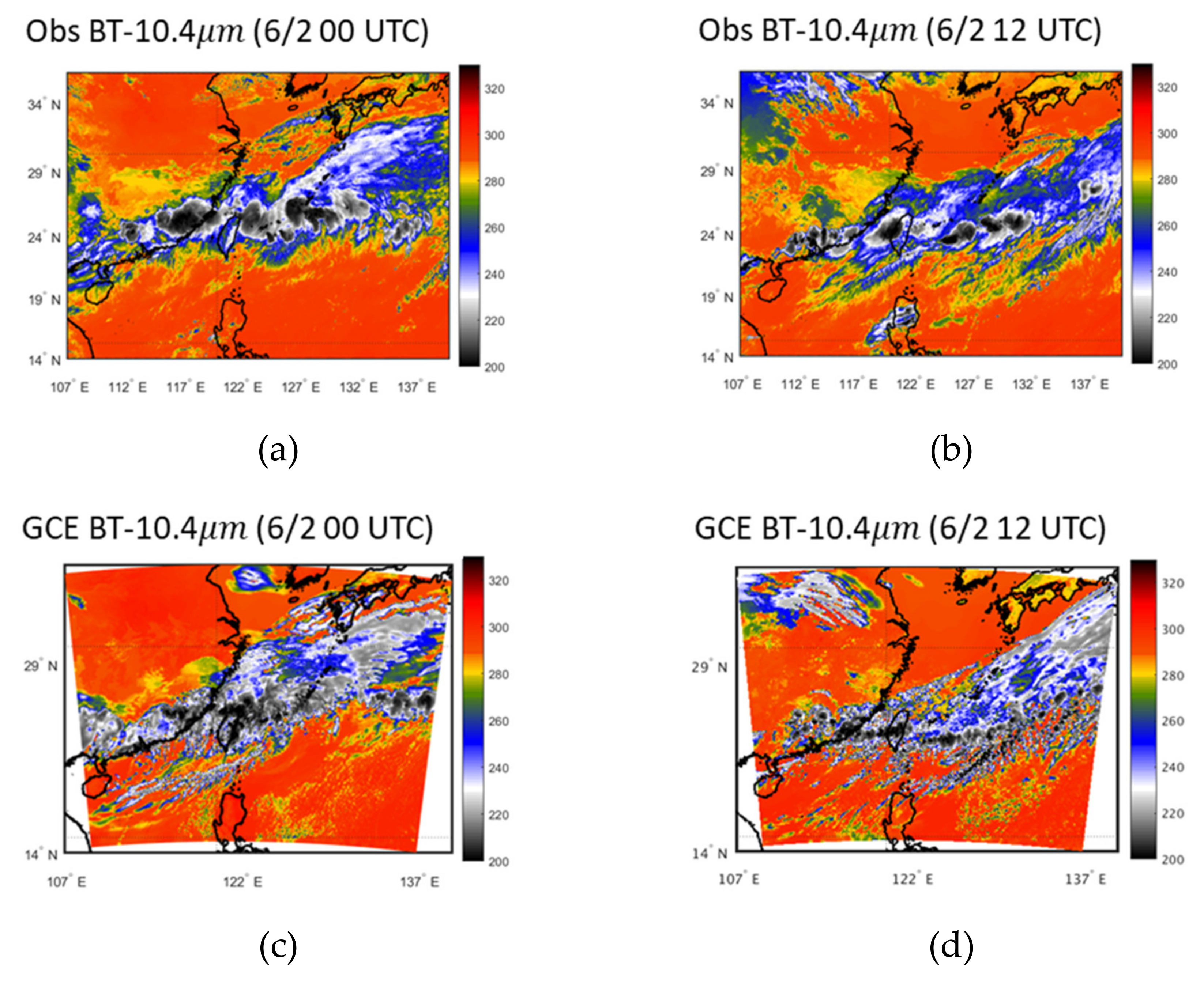
4.2.1. Atmospheric Window Channel (10.4 µm) BT

Figure 6 displays images of observed and simulated Himawari-8 10.4 µm BTs in domain 2 on June 2 at 0000 and 1200 UTC. Himawari-8 10.4 µm channel is a window channel that can be used to detect cloud and surface features. The position, cloud cover, and temperature at the bottom layer of the numerical model are crucial because the window channels are sensitive to temperature and cloud properties. The simulation run using MOR (Figure 6i,j) resulted in low BT covering with too much high cloud in the domain. The remaining simulations resulted in similar distributions, but some small-scale clouds were displayed in the model run using GCE, which caused the images to be a little grainy. Although the error that is caused by either observation or forward model was not considered in the present study (Figure 6), only the relative differences among the forward model calculations and observation are the main concern but not the absolute values in the simulated BTs from forward calculation.

On June 2 at 0000 UTC (12-h simulation), all four model simulations exhibited a cold bias at the East China Sea, which might be correlated to either a larger frontal system coverage or higher altitude in clouds against to the observed BT. Furthermore, the movement of the cloud bands may be slightly delayed. Since the atmospheric factors may bias BTs, the result indicates that the model cannot completely represent the atmospheric conditions. The 24-h simulation, valid on June 2 at 1200 UTC, using the MOR scheme displayed similar characteristics in the 12-h simulation. Approximately half of the MOR D02 displayed a cold bias because of excess cloud cover in the simulation. The simulations with GCE (Figure 6d), WSM (Figure 6f), and WDM (Figure 6h) displayed improved main cloud patterns. However, a cold bias over the south of Japan and the upper left of the domain revealed that the models may generate an excess of cloudy pixels.

Figure 7 displays the BT histograms of the probability of occurrence using the four microphysical scheme model simulations and the corresponding satellite observations. The BT histogram focuses on the distribution of BTs to enable the suppression of the error caused by the weather system location. The probability of occurrence, valid on June 2, 2017 at 0000 UTC and 1200 UTC is presented in Figure 7a,b, respectively. The observations revealed that the highest probability of occurrence occurred at approximately 292 K. However, the simulations with four microphysical schemes all displayed the highest probability at higher BT. The BT of the window channel was >285 K, which suggests low cloud or clear sky, and thus the maximum probability of occurrence appears at higher BT, which indicates that each scheme underestimated the cloud-top height or that the surface temperature was positively biased. A BT of <235 K suggests a high cloud case. A higher probability of high cloud was observed in all four schemes comparing with the observation, suggesting an overestimation of high cloud, especially in the model run using the MOR scheme comparing among the four model configurations.

Furthermore, results indicated that the performance of WSM and WDM displayed similar BT distributions. When the BT was <270 K, the curve of WSM and WDM were almost overlapping. The design of WSM and WDM are similar in the cold rain processes. The results were valid on June 2, 2017 at 1200 UTC (Figure 7b) which indicates that MOR still has too much high cloud cover over domain 2. The observed primary maximum BT was captured by GCE, WDM, and MOR. However, the model run with MOR underestimates the percentage of the occurrence. The simulated peak of BT with GCE and WDM matches better with observation, compared to WSM. The simulation with WSM and WDM was demonstrated to have a similar distribution of the probability of occurrence when the BT was <270 K.

4.2.2. BTs in Water Vapor Channels

The water vapor channels contain moisture information at various altitudes. Three of the water vapor channels used in this study had distinct vertical weighting functions [60]. The peaks of the weighting functions are at the pressure levels of approximately 340, 440, and 620 hPa, with 6.2, 6.9, and 7.4 µm, respectively. As the weighting at the surface is similar, the verification used the BTD to remove the information close to the surface. Therefore, BTDs between 6.2 and 6.9 and between 6.9 and 7.4 represented the high-level and mid-level water vapor, respectively. The verification was processed when clear pixels were simulated and observed simultaneously.

The high-level water vapor results are illustrated in Figure 8. The results suggest that the numbers of clear pixels are similar in GCE, WSM, and WDM. MAE indicates that the models run using WSM and WDM have very similar performances. The MOR results displayed higher MAE after a 10-h simulation, whereas the GCE results displayed a lower MAE after a 6-h model simulation. The MBE for each simulation revealed a cold bias. The simulation using GCE displayed the lowest MAE and MBE most of the time for both the high-level and mid-level (not shown), which may result in a better water budget.

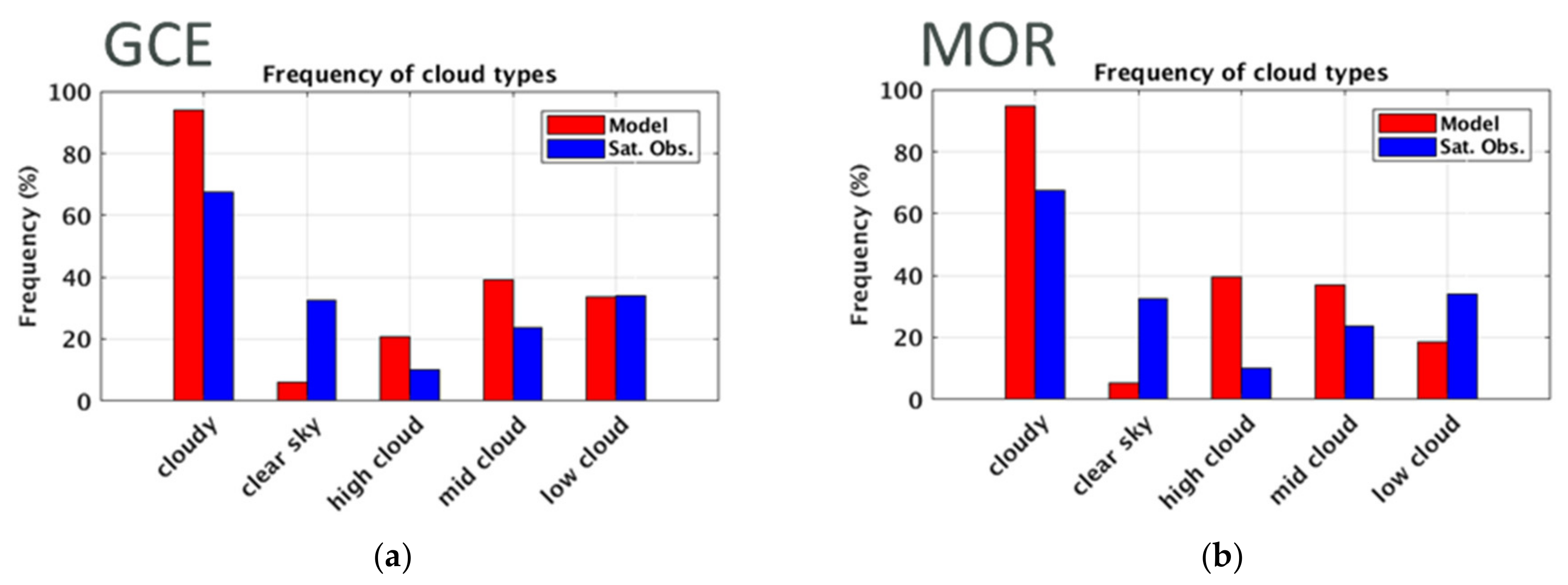
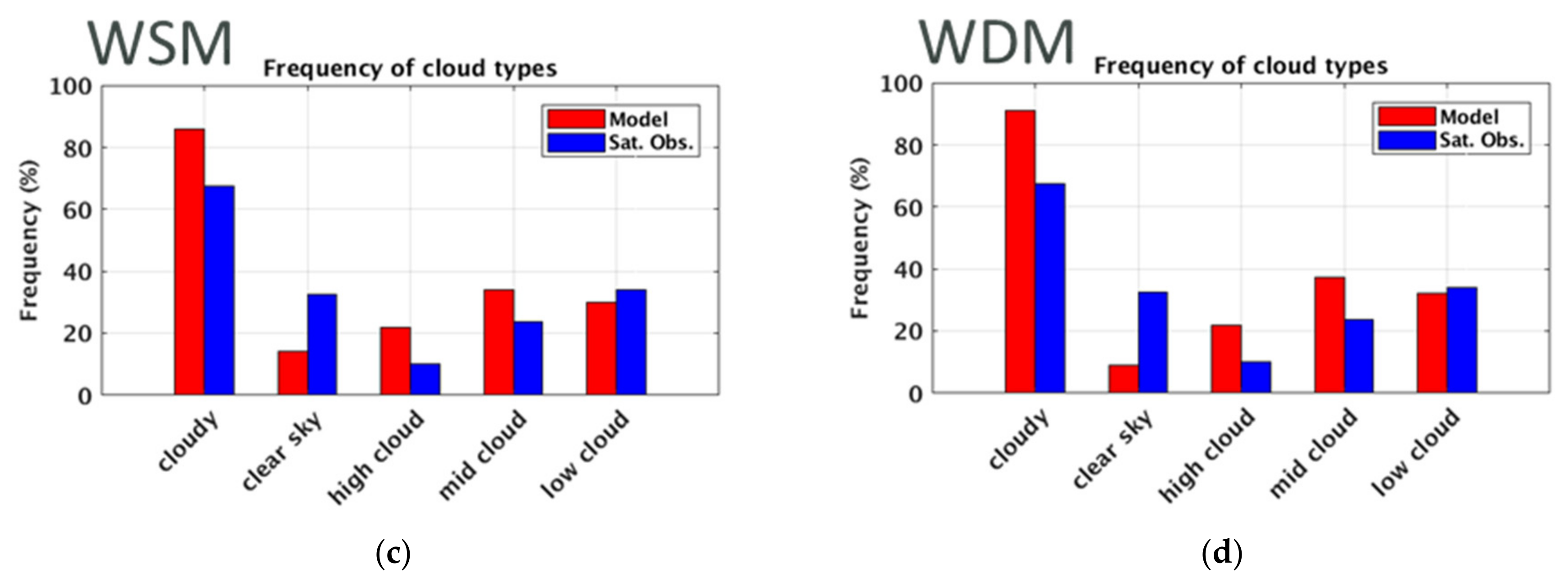
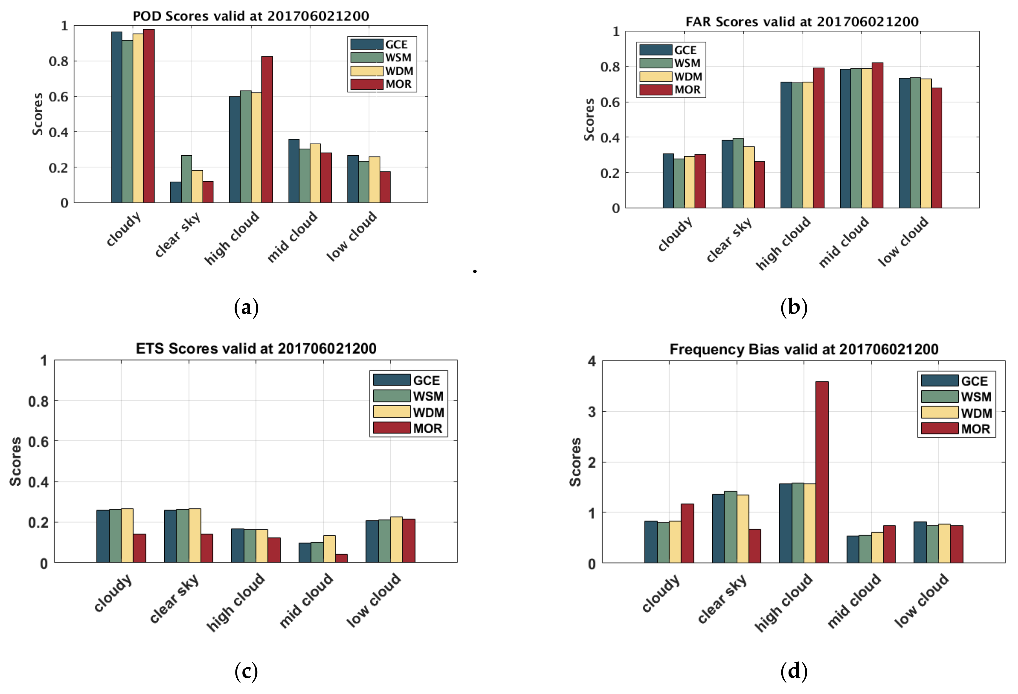
4.2.3. Evaluation of Cloud Types in Model

Figure 9 displays the frequency of each cloud type valid June 2, 2017 at 1200 UTC (24-h simulation). The blue bars represent the results of the observation and the red bars represent the simulations with different microphysical schemes. The results revealed that all four models run overestimated the frequency of cloudy pixels. Excess cloud cover estimates were caused by overestimating high-level and mid-level clouds. An excess of high cloud was produced for the simulation with MOR compared with the observations. GCE, WSM, and WDM adjusted the frequency of low clouds after 24-h simulation compared with the 12-h simulation (not shown).

Figure 10 displays the skill scores of the simulation with different schemes on each cloud type on June 2, 2017 at 1200 UTC. For grid-by-grid evaluation, the results of the POD (Figure 10a) demonstrated that each scheme had a satisfactory performance on cloudy pixels, which indicates that the observed cloudy events were accurately captured by the simulation. When further investigating the cloud types, the high cloud displayed a better performance among the three cloud types. However, overestimation occurred in the cloudy pixel frequency and the POD score ignored false alarms. Therefore, the higher value of POD may not reflect an optimal simulation. The FAR results (Figure 10b) indicated that the value of each cloud type was >0.5, which indicates that at least 50% of simulated events are false alarms. This may be because the exact cloud types were not correct. The ETS score results (Figure 10c) also did not display a high-quality performance on different cloud types. Finally, the FBIASE score (Figure 10d) of the low clouds was near 1, which indicates that the amount of low clouds is closer to the observation at 24-h simulation. Furthermore, the bias of the high cloud for each scheme is >1. In particular, the MOR demonstrated a high cloud bias near 4, which indicated that the presented model estimated approximately four times the cloudy pixels recorded in the corresponding observation.

4.3. Probability Distributions of Hydrometeor Particles

A considerable amount of high clouds was displayed in the simulation with the MOR scheme when verifying the performance of BT. The different hydrometeors were examined because the distribution of hydrometeors may affect the simulation of BT. The probability distributions of cloud ice mixing ratio (Qi) (Figure 11) indicated that the WSM and WDM displayed similar performance. The GCE indicated that the highest mixing ratio of cloud ice was at approximately 8–13 km. However, the distribution of 10.4 µm BT did not perform with the most significant cold bias. On the other hand, the MOR tended to generate more cloud ice at higher altitudes which may contribute to this bias.

4.4. Sensitivity on the Cloud-Top Altitude

In Figure 11, the simulation with GCE had the highest mixing ratio of Qi but did not cover with more cold bias of BT in the model domain compared with other simulations. However, overestimation of the high cloud and a higher Qi at higher altitudes were demonstrated in the simulation with the MOR scheme. Therefore, we assumed that the overestimation of the high cloud with the MOR was affected by the distribution of Qi being too high. To verify this hypothesis, a sensitivity test experiment was designed to examine the influence of the vertical distribution of hydrometeors. To lower the distribution of the hydrometeors by a number of levels, the effective radius and water content of hydrometeors simulated by WRF with MOR was moved directly downwards by removing the bottom layers of the hydrometeors, so that the height on the number concentration (Ni) corresponded to the level of Qi. To maintain the numbers of vertical layers, the uppermost layers were assumed to have no hydrometeors. The reconstructed atmosphere was used as input to the radiative transfer model to compute the BTs. The experiment was designed to compare two parts: Experiment 1 was “Qi only”, in which only the height of the cloud ice effective radius and ice water content was controlled; Experiment 2 was “All”, in which the heights of all hydrometeors were simultaneously controlled.

The MAE and MBE were used to verify the improvements in the high cloud produced by MOR. The results of the MAE and MBE (Figure 12) indicated that lowering the height of all hydrometeors by 4–5 layers led to the largest improvements. However, lowering the height of Qi only resulted in similar improvements as lowering the heights of all hydrometeors. One might notice that the total amount of the hydrometeor might not conserve in the experiment, the results of two sensitivity tests (Figure 12) suggested that Qi was the most crucial factor in the overestimation of the “high cloud” for the MOR scheme.

4.5. Evaluation of the Cloud Pattern Evolution

The synoptic-scale cloud features and the water vapor channel revealed the performance of the simulation using each scheme. In this subsection, the model simulations at domain 3 (3-km horizontal resolution) which focus on the main cloud band for the precipitation system event near the Taiwan are compared with high-resolution satellite observation to verify the performance of each scheme on the main cloud band.

Roebber [61] illustrated an alternative approach to demonstrate multiple verification measures called the “performance diagram” which uses the success ratio (i.e., the value of 1-FAR) as the horizontal axis and the POD score as the vertical axis to illustrate the performance. Moreover, because of the mathematical correspondence, the slope of the dotted line represents FBIAS and the shaded background represents TS.

Figure 13 demonstrates multiple verification measures of simulation accuracy on the performance diagram. Each figure illustrates the simultaneous performance of various cloud classifications and skill scores. The perfect performance will make the dot display in the top-right corner.

The verification results suggest that the improved skill could be identified in the cloudy pixels. In particular, a higher TS and a close to 1 FBIAS value with the simulation using the MOR scheme, indicates that this scheme has less deviation and is closer to the observation. However, this part of the verification only focused on the main cloud area and thus the simulation using the MOR scheme displayed the most favorable performance. The verification of clear pixels revealed that GCE, WSM, and WDM overestimated the clear pixels, whereas MOR underestimated it slightly after the 6-h simulation. Furthermore, the verification results of different cloud types revealed that each model simulation displayed a superior performance on high cloud pixels. The performance of the simulation of low clouds was initially poor, but the verification score rises after 18-h simulation. This might be because the convections in the frontal system were weakening after 18 h from initialization of model. Thus, an improved skill in later stage of low cloud simulation was identified in the bottom row of Figure 13.

5. Conclusions

The main goal of this study was to assess the performance of model simulation objectively using various microphysical schemes. To this end, new-generation multichannel meteorological geostationary satellite observations were used as the reference. The model evaluation using higher spatiotemporal satellite observations could be considered an optimal and comprehensive method. We combined an NWP model (i.e., WRF) and the CRTM to simulate the multichannel BTs from the AHI onboard the Himawari-8 geostationary satellite. Therefore, the entire NWP model domain could be evaluated in an advanced method by comparing the simulated BTs to observations.

A classical stationary front in the Mei-Yu season in Taiwan on June 1–3, 2017, was simulated by WRF using four different microphysical schemes, which includes two single-moment schemes (GCE and WSM) and two double-moment schemes (WDM and MOR). The results of each model simulation using different microphysical schemes revealed that they captured the dynamic and thermodynamic meteorological field (i.e., the 500-hPa geopotential height synoptic-scale trough on the east of Taiwan, and the ridge over China agrees with the reanalysis data). The model also accurately represented the wind shear and strong temperature gradient over the western Pacific, associated with the frontal system. Compared with the observations, the 24-h model simulation of the total accumulated rainfall predicted the local maximum rainfall patterns accurately across the central and southern mountainous regions. Overall, the results of the synoptic conditions and total accumulated rainfall indicated that the WRF simulation with four MP schemes represented this event accurately and similarly qualitatively.

Comparison between simulated and observed BTs provided the following results:

• In the 10.4 μm BT, the results revealed a large cold bias in the simulation using MOR, which was caused by modeling the clouds at higher altitudes. The simulations with GCE, WSM, and WDM captured the distribution of the main cloud band more accurately. The probability of occurrence indicated excessive high cloud occurrences in the simulation with each scheme, and especially in the model run using MOR. The performance of WSM and WDM had similar BTs distributions when the BT was <270 K, which may be because WSM and WDM only differ for warm cloud processes.
• The grid-by-grid evaluation revealed that observed cloudy events were accurately captured by the simulation using four schemes. Furthermore, high cloud pixels displayed a higher accuracy than mid and low clouds.
• The moisture information from clear pixels indicated that the mean bias was positive in the middle layer (approximately 620–420 hPa) and negative in the upper layer (approximately 420–340 hPa). GCE displayed a lower MAE and MBE in most instances, which may result in a better water budget.

Overall, this study demonstrated the potential of WRF coupled with CRTM in producing multichannel satellite imagery as a model performance evaluation tool. The satellite observations provided wide spatial coverage data, which are useful in comprehensively evaluating the NWP models. As only one case was analyzed, some results might be not robust in the present study. The characteristics of these microphysical schemes in different weather systems (e.g., mesoscale typhoon, afternoon thunderstorm, etc.) or the long-term evaluation (e.g., ≥15-day simulation) will be examined in future studies, since the evaluation system has been constructed. Moreover, the effect of other physical parameterization methods in WRF over East Asia can be evaluated from the perspective of radiance. Furthermore, a recent study (e.g., [62]) revealed that the microphysical properties and optical characteristics of the clouds could be estimated from the geostationary orbit. The WRF simulated hydrometers variables may have direct intercomparison against to satellite retrievals, so that the microphysical scheme might be enhanced through the optimal turning from the synergistic analysis between models and satellite data sets.

References

1. Karl, T.R.; Jones, P.D.; Knight, R.W.; Kukla, G.; Plummer, N.; Razuvayev, V.; Gallo, K.P.; Lindseay, J.; Charlson, R.J.; Peterson, T.C. A New Perspective on Recent Global Warming: Asymmetric Trends of Daily Maximum and Minimum Temperature. Bull. Am. Meteorol. Soc. 1993, 74, 1007–1024. [Google Scholar] [CrossRef] [Green Version]
2. Dai, A.; Trenberth, K.E.; Karl, T.R. Effects of Clouds, Soil Moisture, Precipitation, and Water Vapor on Diurnal Temperature Range. J. Clim. 1999, 12, 2451–2473. [Google Scholar] [CrossRef]
3. Ramanathan, V. The role of earth radiation budget studies in climate and general circulation research. J. Geophys. Res. Atmos. 1987, 92, 4075–4095. [Google Scholar] [CrossRef]
4. Arking, A. The Radiative Effects of Clouds and their Impact on Climate. Bull. Am. Meteorol. Soc. 1991, 72, 795–814. [Google Scholar] [CrossRef]
5. Mecikalski, J.R.; Bedka, K.M. Forecasting Convective Initiation by Monitoring the Evolution of Moving Cumulus in Daytime GOES Imagery. Mon. Weather Rev. 2006, 134, 49–78. [Google Scholar] [CrossRef] [Green Version]
6. Sieglaff, J.M.; Cronce, L.M.; Feltz, W.F.; Bedka, K.M.; Pavolonis, M.J.; Heidinger, A.K. Nowcasting Convective Storm Initiation Using Satellite-Based Box-Averaged Cloud-Top Cooling and Cloud-Type Trends. J. Appl. Meteorol. Climatol. 2011, 50, 110–126. [Google Scholar] [CrossRef]
7. Cintineo, J.L.; Pavolonis, M.J.; Sieglaff, J.M.; Heidinger, A.K. Evolution of Severe and Nonsevere Convection Inferred from GOES-Derived Cloud Properties. J. Appl. Meteorol. Climatol. 2013, 52, 2009–2023. [Google Scholar] [CrossRef]
8. Tripoli, G.J.; Cotton, W.R. Numerical Study of an Observed Orogenic Mesoscale Convective System. Part 2: Analysis of Governing Dynamics. Mon. Weather Rev. 1989, 117, 305–328. [Google Scholar] [CrossRef] [Green Version]
9. Tao, W.-K.; Moncrieff, M.W. Multiscale cloud system modeling. Rev. Geophys. 2009, 47. [Google Scholar] [CrossRef] [Green Version]
10. Satoh, M.; Inoue, T.; Miura, H. Evaluations of cloud properties of global and local cloud system resolving models using CALIPSO and CloudSat simulators. J. Geophys. Res. Atmos. 2010, 115. [Google Scholar] [CrossRef]
11. Jankov, I.; Bao, J.-W.; Neiman, P.J.; Schultz, P.J.; Yuan, H.; White, A.B. Evaluation and Comparison of Microphysical Algorithms in ARW-WRF Model Simulations of Atmospheric River Events Affecting the California Coast. J. Hydrometeorol. 2009, 10, 847–870. [Google Scholar] [CrossRef]
12. Jung, Y.; Xue, M.; Zhang, G. Simulations of Polarimetric Radar Signatures of a Supercell Storm Using a Two-Moment Bulk Microphysics Scheme. J. Appl. Meteorol. Climatol. 2010, 49, 146–163. [Google Scholar] [CrossRef]
13. Otkin, J.A.; Greenwald, T.J. Comparison of WRF Model-Simulated and MODIS-Derived Cloud Data. Mon. Weather Rev. 2008, 136, 1957–1970. [Google Scholar] [CrossRef]
14. Cintineo, R.; Otkin, J.A.; Xue, M.; Kong, F. Evaluating the Performance of Planetary Boundary Layer and Cloud Microphysical Parameterization Schemes in Convection-Permitting Ensemble Forecasts Using Synthetic GOES-13 Satellite Observations. Mon. Weather Rev. 2014, 142, 163–182. [Google Scholar] [CrossRef] [Green Version]
15. Randel, D.L.; Haar, T.H.V.; Ringerud, M.A.; Stephens, G.L.; Greenwald, T.J.; Combs, C.L. A New Global Water Vapor Dataset. Bull. Am. Meteorol. Soc. 1996, 77, 1233–1246. [Google Scholar] [CrossRef] [Green Version]
16. Schaaf, C.B.; Gao, F.; Strahler, A.H.; Lucht, W.; Li, X.; Tsang, T.; Strugnell, N.C.; Zhang, X.; Jin, Y.; Muller, J.-P.; et al. Roy, First operational BRDF, albedo nadir reflectance products from MODIS. Remote Sens. Environ. 2002, 83, 135–148. [Google Scholar] [CrossRef] [Green Version]
17. Wiedner, M.; Prigent, C.; Pardo, J.R.; Nuissier, O.; Chaboureau, J.-P.; Pinty, J.-P.; Mascart, P. Modeling of passive microwave responses in convective situations using output from mesoscale models: Comparison with TRMM/TMI satellite observations. J. Geophys. Res. Atmos. 2004, 109. [Google Scholar] [CrossRef]
18. Liu, C.-Y.; Li, J.; Ho, S.; Liu, G.; Lin, T.; Young, C. Retrieval of Atmospheric Thermodynamic State From Synergistic Use of Radio Occultation and Hyperspectral Infrared Radiances Observations. IEEE J. Sel. Top. Appl. Earth Obs. Remote Sens. 2016, 9, 744–756. [Google Scholar] [CrossRef]
19. Morcrette, J.-J. Evaluation of model-generated cloudiness: Satellite-observed and model-generated diurnal variability of brightness temperature. Mon. Weather Rev. 1991, 119, 1205–1224. [Google Scholar] [CrossRef] [Green Version]
20. Chaboureau, J.-P.; Nuissier, O.; Claud, C. Verification of ensemble forecasts of Mediterranean high-impact weather events against satellite observations. Nat. Hazards Earth Syst. Sci. 2012, 12. [Google Scholar] [CrossRef]
21. Greenwald, T.J.; Lee, Y.-K.; Otkin, J.A.; L’Ecuyer, T. Evaluation of midlatitude clouds in a large-scale high-resolution simulation using CloudSat observations. J. Geophys. Res. Atmos. 2010, 115. [Google Scholar] [CrossRef] [Green Version]
22. Yu, W.; Sèze, G.; Le Treut, H.; Desbois, M. Desbois, and Oceans, Comparison of radiance fields observed by satellite and simulated by the LMD general circulation model. Dyn. Atmos. 1991, 16, 147–165. [Google Scholar] [CrossRef]
23. Griffin, S.M.; Otkin, J.A.; Rozoff, C.M.; Sieglaff, J.M.; Cronce, L.M.; Alexander, C.R. Methods for comparing simulated and observed satellite infrared brightness temperatures and what do they tell us? Weather Forecast. 2017, 32, 5–25. [Google Scholar] [CrossRef]
24. Diaz, J.P.; González, A.; Expósito, F.J.; Pérez, J.C.; Fernández, J.; García-Díez, M.; Taima, D. WRF multi-physics simulation of clouds in the African region. Q. J. R. Meteorol. Soc. 2015, 141, 2737–2749. [Google Scholar] [CrossRef]
25. Zhang, Y.; Rockel, B.; Stuhlmann, R.; Hollmann, R.; Karstens, U. REMO Cloud Modeling: Improvements and Validation with ISCCP DX Data. J. Appl. Meteorol. 2001, 40, 389–408. [Google Scholar] [CrossRef]
26. Chaboureau, J.P.; Pinty, J.P. Validation of a cirrus parameterization with Meteosat Second Generation observations. Geophys. Res. Lett. 2006, 33. [Google Scholar] [CrossRef] [Green Version]
27. Pincus, R.; Batstone, C.P.; Hofmann, R.J.P.; Taylor, K.E.; Glecker, P.J. Evaluating the present-day simulation of clouds, precipitation, and radiation in climate models. J. Geophys. Res. Atmos. 2008, 113. [Google Scholar] [CrossRef]
28. Otkin, J.A.; Greenwald, T.J.; Sieglaff, J.; Huang, H.-L. Validation of a Large-Scale Simulated Brightness Temperature Dataset Using SEVIRI Satellite Observations. J. Appl. Meteorol. Climatol. 2009, 48, 1613–1626. [Google Scholar] [CrossRef]
29. Liang, X.-M.; Ignatov, A.; Kihai, Y. Implementation of the Community Radiative Transfer Model in Advanced Clear-Sky Processor for Oceans and validation against nighttime AVHRR radiances. J.Geophys. Res. Atmos. 2009, 114. [Google Scholar] [CrossRef]
30. Bedka, K.; Brunner, J.; Dworak, R.; Feltz, W.; Otkin, J.; Greenwald, T. Objective Satellite-Based Detection of Overshooting Tops Using Infrared Window Channel Brightness Temperature Gradients. J. Appl. Meteorol. Climatol. 2010, 49, 181–202. [Google Scholar] [CrossRef]
31. Roh, W.; Satoh, M.; Nasuno, T. Improvement of a Cloud Microphysics Scheme for a Global Nonhydrostatic Model Using TRMM and a Satellite Simulator. J. Atmos. Sci. 2017, 74, 167–184. [Google Scholar] [CrossRef]
32. Matsui, T.; Chern, J.-D.; Tao, W.-K.; Lang, S.; Satoh, M.; Hashino, T.; Kubota, T. On the Land–Ocean Contrast of Tropical Convection and Microphysics Statistics Derived from TRMM Satellite Signals and Global Storm-Resolving Models. J. Hydrometeorol. 2016, 17, 1425–1445. [Google Scholar] [CrossRef] [PubMed]
33. Li, Y.; Zipser, E.J.; Krueger, S.K.; Zulauf, M.A. Cloud-Resolving Modeling of Deep Convection during KWAJEX. Part I: Comparison to TRMM Satellite and Ground-Based Radar Observations. Mon. Weather Rev. 2008, 136, 2699–2712. [Google Scholar] [CrossRef] [Green Version]
34. Grasso, L.D.; Sengupta, M.; Demaria, M. Comparison between observed and synthetic 6.5 and 10.7 μm GOES-12 imagery of thunderstorms that occurred on 8 May 2003. Int. J. Remote Sens. 2010, 31, 647–663. [Google Scholar] [CrossRef]
35. Jankov, I.; Grasso, L.D.; Sengupta, M.; Neiman, P.J.; Zupanski, D.; Zupanski, M.; Lindsey, D.; Hillger, D.W.; Birkenheuer, D.L.; Brummer, R. An evaluation of five ARW-WRF microphysics schemes using synthetic GOES imagery for an atmospheric river event affecting the California coast. J. Hydrometeorol. 2011, 12, 618–633. [Google Scholar] [CrossRef] [Green Version]
36. Liu, C.-Y.; Lin, M.-Y.; Chen, J.-H.; Chang, M.-Y.; Chang, T.-H. Objective Evaluation of Numerical Weather Model Forecasts by Using Satellite-Observed Radiances. IEEE Tgrs. 2020. (under review). [Google Scholar]
37. Yao, B.; Liu, C.; Yin, Y.; Zhang, P.; Min, M.; Han, W. Radiance-based evaluation of WRF cloud properties over East Asia: Direct comparison with FY-2E observations. J. Geophys. Res. Atmos. 2018, 123, 4613–4629. [Google Scholar] [CrossRef]
38. Chung, K.-S.; Chang, W.; Fillion, L.; Tanguay, M. Examination of Situation-Dependent Background Error Covariances at the Convective Scale in the Context of the Ensemble Kalman Filter. Mon. Weather Rev. 2013, 141, 3369–3387. [Google Scholar] [CrossRef]
39. Tu, C.-C.; Chen, Y.-L.; Lin, P.-L.; Lin, P.-H. The relationship between the boundary layer moisture transport from the South China Sea and heavy rainfall over Taiwan. Terr. Atmos. Ocean. Sci. 2020, 31, 159–176. [Google Scholar] [CrossRef]
40. Lupo, K.M.; Torn, R.D.; Yang, S.-C. Evaluation of Stochastic Perturbed Parameterization Tendencies on Convective-Permitting Ensemble Forecasts of Heavy Rainfall Events in New York and Taiwan. Weather Forecast. 2019, 35, 5–24. [Google Scholar] [CrossRef]
41. Yeh, H.-C.; Chen, G.T.-J. Case study of an unusually heavy rain event over eastern Taiwan during the Mei-yu season. Mon. Weather Rev. 2004, 132, 320–337. [Google Scholar] [CrossRef]
42. Geng, B. Case study of a split front and associated precipitation during the mei-yu season. Weather Forecast. 2014, 29, 996–1002. [Google Scholar] [CrossRef]
43. Ke, C.-Y.; Chung, K.-S.; Wang, T.-C.C.; Liou, Y.-C. Analysis of heavy rainfall and barrier-jet evolution during Mei-Yu season using multiple Doppler radar retrievals: A case study on 11 June 2012. Tellus A Dyn. Meteorol. Oceanogr. 2019, 71, 1571369. [Google Scholar] [CrossRef] [Green Version]
44. Morel, C.; Senesi, S. A climatology of mesoscale convective systems over Europe using satellite infrared imagery. II: Characteristics of European mesoscale convective systems. Q. J. R. Meteorol. Soc. J. Atmos. Sci. Appl. Meteorol. Phys. Oceanogr. 2002, 128, 1973–1995. [Google Scholar] [CrossRef]
45. Parker, M.D.; Johnson, R.H. Organizational modes of midlatitude mesoscale convective systems. Mon. Weather Rev. 2000, 128, 3413–3436. [Google Scholar] [CrossRef]
46. Mlawer, E.J.; Taubman, S.J.; Brown, P.D.; Iacono, M.J.; Clough, S.A. Radiative transfer for inhomogeneous atmospheres: RRTM, a validated correlated-k model for the longwave. J. Geophys. Res. Atmos. 1997, 102, 16663–16682. [Google Scholar] [CrossRef] [Green Version]
47. Dudhia, J. Numerical study of convection observed during the winter monsoon experiment using a mesoscale two-dimensional model. J. Atmos. Sci. 1989, 46, 3077–3107. [Google Scholar] [CrossRef]
48. Hong, S.-Y.; Noh, Y.; Dudhia, J. A new vertical diffusion package with an explicit treatment of entrainment processes. Mon. Weather Rev. 2006, 134, 2318–2341. [Google Scholar] [CrossRef] [Green Version]
49. Kain, J.S. The Kain–Fritsch Convective Parameterization: An Update. J. Appl. Meteorol. 2004, 43, 170–181. [Google Scholar] [CrossRef] [Green Version]
50. Tao, W.-K.; Simpson, J.; Baker, D.; Braun, S.; Chou, M.-D.; Ferrier, B.; Johnson, D.; Khain, A.; Lang, S.; Lynn, B.; et al. Microphysics, radiation and surface processes in the Goddard Cumulus Ensemble (GCE) model. Theor. Appl. Clim. 2003, 82, 97–137. [Google Scholar] [CrossRef]
51. Hong, S.-Y.; Lim, J.-O.J. The WRF single-moment 6-class microphysics scheme (WSM6). Asia Pac. J. Atmos. Sci. 2006, 42, 129–151. [Google Scholar]
52. Lim, K.-S.S.; Hong, S.-Y. Development of an effective double-moment cloud microphysics scheme with prognostic cloud condensation nuclei (CCN) for weather and climate models. Mon. Weather Rev. 2010, 138, 1587–1612. [Google Scholar] [CrossRef] [Green Version]
53. Morrison, H.; Curry, J.; Khvorostyanov, V. A new double-moment microphysics parameterization for application in cloud and climate models. Part I: Description. J. Atmos. Sci. 2005, 62, 1665–1677. [Google Scholar] [CrossRef]
54. Bessho, K.; Date, K.; Hayashi, M.; Ikeda, A.; Imai, T.; Inoue, H.; Kumagai, Y.; Miyakawa, T.; Murata, H.; Ohno, T.; et al. An Introduction to Himawari-8/9— Japan’s New-Generation Geostationary Meteorological Satellites. J. Meteorol. Soc. Japan. Ser. Ii 2016, 94, 151–183. [Google Scholar] [CrossRef] [Green Version]
55. Murata, H.; Takahashi, M.; Kosaka, Y. VIS and IR bands of Himawari-8/AHI compatible with those of MTSAT-2/Imager. Msc Tech. Note 2015, 60, 1–18. [Google Scholar]
56. Ding, S.; Yang, P.; Weng, F.; Liu, Q.; Han, Y.; van Delst, P.; Li, J.; Baum, B. Validation of the community radiative transfer model. J. Quant. Spectrosc. Radiat. Transf. 2011, 112, 1050–1064. [Google Scholar] [CrossRef]
57. Martin, G.M.; Johnson, D.W.; Spice, A. The Measurement and Parameterization of Effective Radius of Droplets in Warm Stratocumulus Clouds. J. Atmos. Sci. 1994, 51, 1823–1842. [Google Scholar] [CrossRef]
58. Hong, S.-Y.; Dudhia, J.; Chen, S.-H. A Revised Approach to Ice Microphysical Processes for the Bulk Parameterization of Clouds and Precipitation. Mon. Weather Rev. 2004, 132, 103–120. [Google Scholar] [CrossRef]
59. Wilks, D.S. Statistical Methods in the Atmospheric Sciences, 2nd ed.; Academic Press: Cambridge, MA, USA, 2006; p. 627. [Google Scholar]
60. Wu, Y.; Zhang, F.; Wu, K.; Min, M.; Li, W.; Liu, R. Best Water Vapor Information Layer of Himawari-8-Based Water Vapor Bands over East Asia. Sensors 2020, 20, 2394. [Google Scholar] [CrossRef] [Green Version]
61. Roebber, P.J. Visualizing multiple measures of forecast quality. Weather Forecast. 2009, 24, 601–608. [Google Scholar] [CrossRef] [Green Version]
62. Liu, C.-Y.; Chiu, C.-H.; Lin, P.-H.; Min, M. Comparison of Cloud-Top Property Retrievals from Advanced Himawari Imager, MODIS, CloudSat/CPR, CALIPSO/CALIOP, and radiosonde. J. Geophys. Res. Atmos. 2020, 125, e2020JD032683. [Google Scholar] [CrossRef]
Figure 1. The composited radar reflectivity. Valid on (a) June 1, 2017 at 1800 UTC; (b) June 1, 2017 at 2100 UTC; (c) June 2, 2017 at 0000 UTC; (d) June 2, 2017 at 0300 UTC.
Remotesensing 12 03060 g001
Figure 2. Illustration of domain coverage in D01, D02, and D03. The horizontal resolution was 27, 9, and 3 km in D01 to D03, respectively.
Remotesensing 12 03060 g002
Figure 3. Illustration of the cloud classification process.
Remotesensing 12 03060 g003
Figure 4. Weather chart of the reanalysis (a,c,e) and GCE (b,d,f) at 500 and 850 hPa and at the surface. Valid on 02 June 2017at 1200 UTC.
Remotesensing 12 03060 g004aRemotesensing 12 03060 g004b
Figure 5. Total rainfall accumulation (mm) from June 1 at 1200 UTC to June 2 at 1200 UTC from (a) observation and (b) simulation with GCE in domain 3.
Remotesensing 12 03060 g005
Figure 6. The observed (a,b) and simulated (cj) BT on 2 June 2017 at 0000 and 1200 UTC.
Remotesensing 12 03060 g006aRemotesensing 12 03060 g006b
Figure 7. Domain 02 BT 10.4 µm probability of occurrence valid on 2 June 2017 at (a) 0000 and (b) 1200 UTC.
Remotesensing 12 03060 g007
Figure 8. Number of clear pixels (a) in MAE (b) and MBE (c) of high-level water vapor. The horizontal axis is the valid time.
Remotesensing 12 03060 g008aRemotesensing 12 03060 g008b
Figure 9. Frequency of cloud type. Valid on June 2 at 1200 UTC and simulated with (a) GCE, (b) MOR, (c) WSM, and (d) WDM.
Remotesensing 12 03060 g009aRemotesensing 12 03060 g009b
Figure 10. Skill score of each cloud type. Valid on June 2 at 1200 UTC. (a) POD, (b) FAR, (c) ETS, and (d) FBIAS.
Remotesensing 12 03060 g010
Figure 11. Probability distributions of Qi simulated with (a) GCE, (b) MOR, (c) WSM, and (d) WDM. The shaded color displays the probability at each altitude. The simulation is initial at 060112 UTC and valid at 06021200 UTC.
Remotesensing 12 03060 g011
Figure 12. MAE and MBE for 10.4 µm BT of high cloud. Valid on June 2, 2017 at 1200 UTC. (a) Qi only and (b) All.
Remotesensing 12 03060 g012
Figure 13. Performance diagram of 24-h simulation. The color of dots indicates the simulation time steps starting from 1 June 2017 at 1300 UTC to 2 June 2017 at 1200 UTC at 1-h intervals. Each row illustrates the performance of different cloud top types and each column indicates the simulation using each MP scheme.
Remotesensing 12 03060 g013