Evaluating the Performance of a Convection-Permitting Model by Using Dual-Polarimetric Radar Parameters: Case Study of SoWMEX IOP8


Abstract
1. Introduction
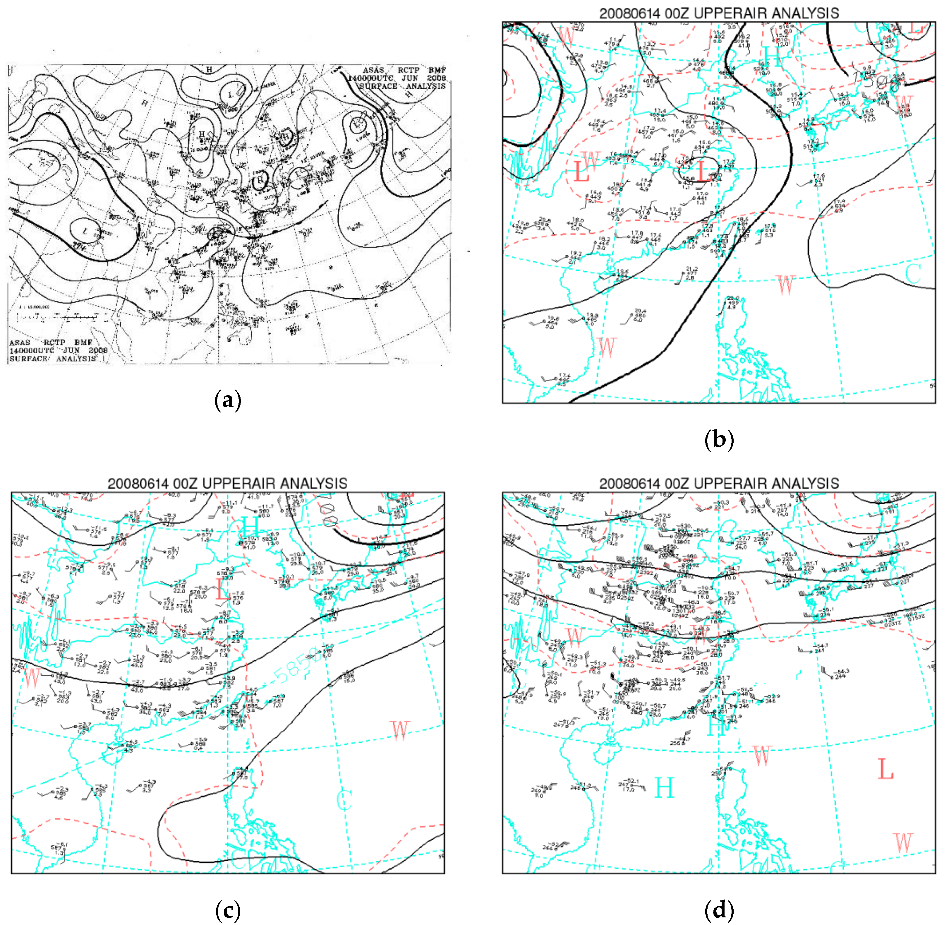
2. Case Overview
3. Methodology and Experiment Design
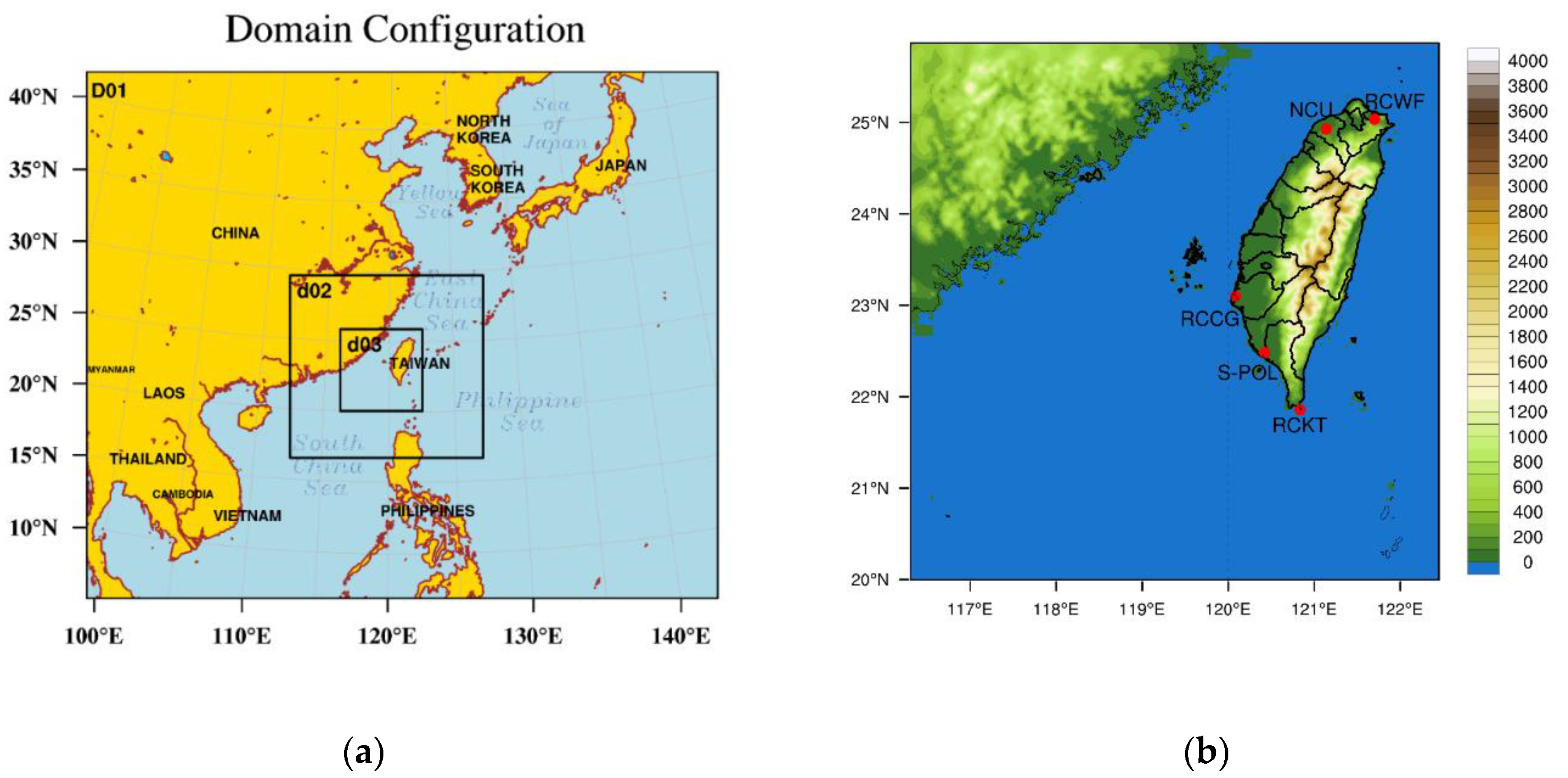
3.1. Model Configuration
3.2. WRF Local Ensemble Transform Kalman Filter Radar Assimilation System (WLRAS)
3.3. Radar Data QC and Process
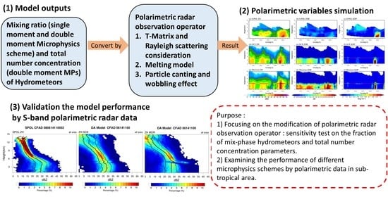
3.4. Observation Operator
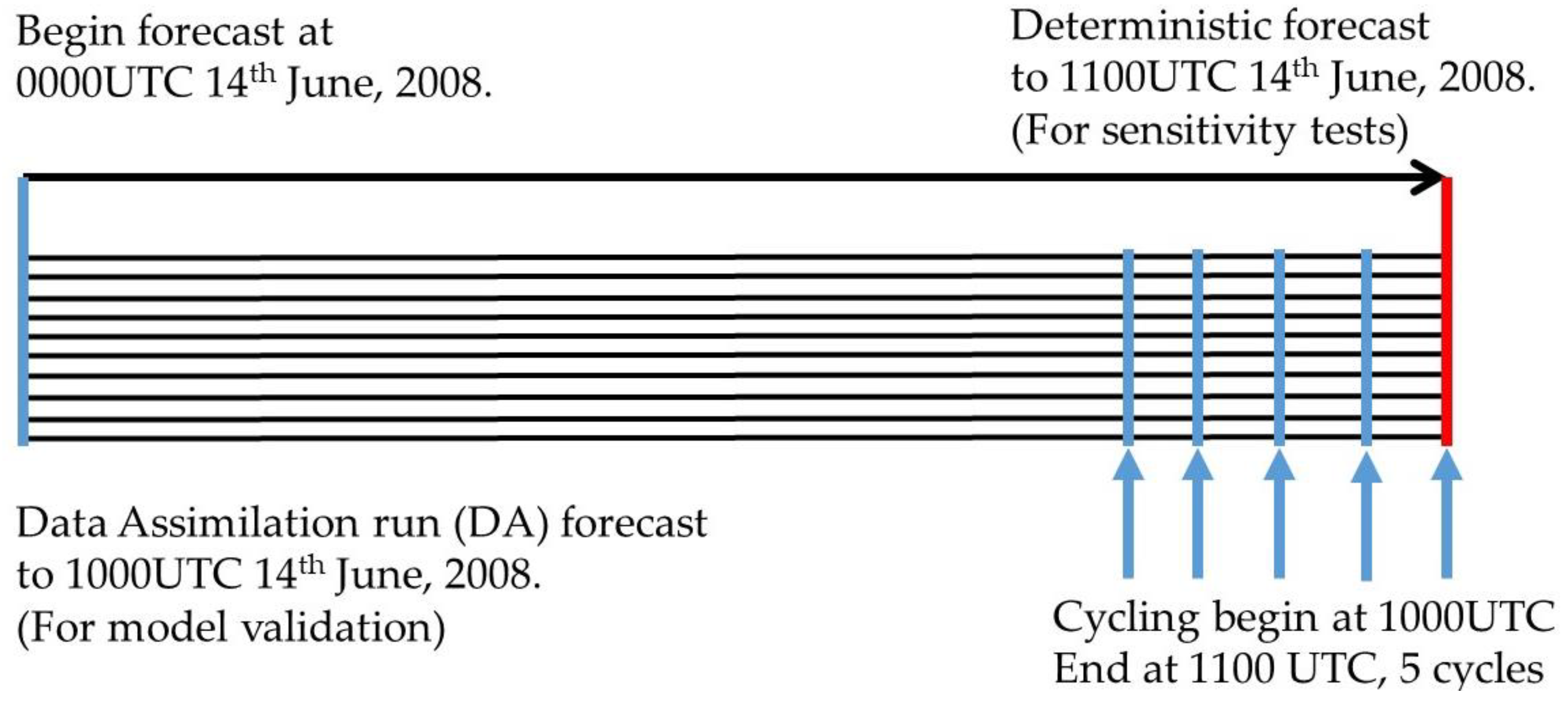
3.5. Experimental Design
4. Results
4.1. Sensitivity Tests of the Operator
4.2. Performance of the Analysis Against the S-POL
4.3. Statistical Verification of System Structure Using the CFAD
4.4. Inspection of the Differences in Microphysics
4.5. Histograms
5. Discussion
6. Conclusions
Author Contributions
Funding
Acknowledgments
Conflicts of Interest
References
- Houze, R.A.; Rutledge, S.A., Jr.; Biggerstaff, M.I.; Smull, B.F. Interpretation of Doppler weather-radar displays in midlatitude mesoscale convective systems. Bull. Am. Meteorol. Soc. 1989, 70, 608–619. [Google Scholar] [CrossRef]
- Germann, U.; Zawadzki, I. Scale dependence of the predictability of precipitation from continental radar images. Part I: Description of the methodology. Mon. Weather Rev. 2002, 130, 2859–2873. [Google Scholar] [CrossRef]
- Germann, U.; Zawadzki, I. Scale dependence of the predictability of precipitation from continental radar images. Part II: Probability forecasts. J. Appl. Meteorol. 2004, 43, 74–89. [Google Scholar] [CrossRef]
- Lee, J.-W.; Min, K.-H.; Lee, Y.-H.; Lee, G. X-Net-Based Radar Data Assimilation Study over the Seoul Metropolitan Area. Remote Sens. 2020, 12, 893. [Google Scholar] [CrossRef]
- Sun, J.; Crook, N.A. Dynamical and microphysical retrieval from Doppler radar observations using a cloud model and its adjoint. Part I: Model development and simulated data experiments. J. Atmos. Sci. 1997, 54, 1642–1661. [Google Scholar] [CrossRef]
- Snyder, C.; Zhang, F. Assimilation of simulated Doppler radar observations with an ensemble Kalman filter. Mon. Weather Rev. 2003, 131, 1663–1677. [Google Scholar] [CrossRef]
- Seliga, T.A.; Bringi, V.N. Differential reflectivity and differential phase shift: Applications in radar meteorology. Radio Sci. 1978, 13, 271–275. [Google Scholar] [CrossRef]
- Sachidananda, M.; Zrnić, D.S. Rain rate estimates from differential polarization measurements. J. Atmos. Ocean. Technol. 1987, 4, 588–598. [Google Scholar] [CrossRef]
- Vivekanandan, J.; Zrnic, D.S.; Ellis, S.M.; Oye, R.; Ryzhkov, A.V.; Straka, J. Cloud microphysics retrieval using S-band dual-polarization radar measurements. Bull. Am. Meteorol. Soc. 1999, 80, 381–388. [Google Scholar] [CrossRef]
- Lakshmanan, V.; Karstens, C.; Krause, J.; Tang, L. Quality control of weather radar data using polarimetric variables. J. Atmos. Ocean. Technol. 2014, 31, 1234–1249. [Google Scholar] [CrossRef]
- Kumjian, M.R.; Ryzhkov, A.V. Polarimetric signatures in supercell thunderstorms. J. Appl. Meteorol. Climatol. 2008, 47, 1940–1961. [Google Scholar] [CrossRef]
- Ke, C.-Y.; Chung, K.-S.; Wang, T.-C.C.; Liou, Y.-C. Analysis of heavy rainfall and barrier-jet evolution during Mei-Yu season using multiple doppler radar retrievals: A case study on 11 June 2012. Tellus A Dyn. Meteorol. Oceanogr. 2019, 71, 1571369. [Google Scholar] [CrossRef]
- Morrison, H.; Thompson, G.; Tatarskii, V. Impact of cloud microphysics on the development of trailing stratiform precipitation in a simulated squall line: Comparison of one- and two-moment schemes. Mon. Weather Rev. 2009, 137, 991–1007. [Google Scholar] [CrossRef]
- Hong, S.; Dudhia, J.; Chen, S. A revised approach to ice microphysical processes for the bulk parameterization of clouds and precipitation. Mon. Weather Rev. 2004, 132, 103–120. [Google Scholar] [CrossRef]
- Lin, Y.; Farley, R.D.; Orville, H.D. Bulk parameterization of the snow field in a cloud model. J. Clim. Appl. Meteorol. 1983, 22, 1065–1092. [Google Scholar] [CrossRef]
- Tao, W.K.; Simpson, J.; Baker, D.; Braun, S.; Chou, M.D.; Ferrier, B.; Johnson, D.; Khain, A.; Lang, S.; Lynn, B.; et al. Microphysics, radiation and surface processes in the Goddard Cumulus Ensemble (GCE) model. Meteorol. Atmos. Phys. 2003, 82, 97–137. [Google Scholar] [CrossRef]
- Milbrandt, J.A.; Yau, M.K. A multimoment bulk microphysics parameterization. Part I: Analysis of the role of the spectral shape parameter. J. Atmos. Sci. 2005, 62, 3051–3064. [Google Scholar] [CrossRef]
- Milbrandt, J.A.; Yau, M.K. A multimoment bulk microphysics parameterization. Part II: A proposed three-moment closure and scheme description. J. Atmos. Sci. 2005, 62, 3065–3081. [Google Scholar] [CrossRef]
- Khain, A.; Pokrovsky, A.; Pinsky, M.; Seifert, A.; Phillips, V. 2004 Simulation of effects of atmospheric aerosols on deep turbulent convective clouds using a spectral microphysics mixed-phase cumulus cloud model. Part I: Model description and possible applications. J. Atmos. Sci. 2004, 61, 2963–2982. [Google Scholar] [CrossRef]
- Ulbrich, C.W. Natural variations in the analytical form of the raindrop size distribution. J. Clim. Appl. Meteorol. 1983, 22, 1764–1775. [Google Scholar] [CrossRef]
- Marshall, J.S.; Palmer, W.M.K. The distribution of raindrops with size. J. Meteorol. 1948, 5, 165–166. [Google Scholar] [CrossRef]
- Tokay, A.; Short, D.A. Evidence from tropical raindrop spectra of the origin of rain from stratiform versus convective clouds. J. Appl. Meteorol. 1996, 35, 355–371. [Google Scholar] [CrossRef]
- Bringi, V.N.; Chandrasekar, V.; Hubbert, J.; Gorgucci, E.; Randeu, W.L.; Schoenhuber, M. Raindrop size distribution in different climatic regimes from disdrometer and dual-polarized radar analysis. J. Atmos. Sci. 2003, 60, 354–365. [Google Scholar] [CrossRef]
- Dawson, D.T.; Xue, M.; Milbrandt, J.A.; Yau, M.K. Comparison of evaporation and cold pool development between single-moment and multi-moment bulk microphysics schemes in idealized simulations of tornadic thunderstorms. Mon. Weather Rev. 2010, 138, 1152–1171. [Google Scholar] [CrossRef]
- Putnam, B.J.; Xue, M.; Jung, Y.; Snook, N.; Zhang, G. The analysis and prediction of microphysical states and polarimetric radar variables in a mesoscale convective system using double-moment microphysics, multinetwork radar data, and the ensemble Kalman filter. Mon. Weather Rev. 2014, 142, 141–162. [Google Scholar] [CrossRef]
- Jung, Y.; Zhang, G.; Xue, M. Assimilation of simulated polarimetric radar data for a convective storm using ensemble Kalman filter. Part I: Observation operators for reflectivity and polarimetric variables. Mon. Weather Rev. 2008, 136, 2228–2245. [Google Scholar] [CrossRef]
- Pfeifer, M.; Craig, G.C.; Hagen, M.; Keil, C. A polarimetric radar forward operator for model evaluation. J. Appl. Meteorol. Climatol. 2008, 47, 3202–3220. [Google Scholar] [CrossRef]
- Ryzhkov, A.V.; Pinsky, M.; Pokrovsky, A.; Khain, A.P. Polarimetric radar observation operator for a cloud model with spectral microphysics. J. Appl. Meteorol. Climatol. 2011, 50, 873–894. [Google Scholar] [CrossRef]
- Kumjian, M.R.; Martinkus, C.P.; Prat, O.P.; Collis, S.; van Lier-Walqui, M.; Morrison, H.C. A moment-based polarimetric radar forward operator for rain microphysics. J. Appl. Meteorol. Climatol. 2019, 58, 113–130. [Google Scholar] [CrossRef]
- Jung, Y.; Xue, M.; Zhang, G. Simulations of polarimetric radar signatures of a supercell storm using a two-moment bulk microphysics scheme. J. Appl. Meteorol. Climatol. 2010, 49, 146–163. [Google Scholar] [CrossRef]
- Jung, Y.; Xue, M.; Tong, M. Ensemble Kalman filter analyses of the 29–30 May 2004 Oklahoma tornadic thunderstorm using one- and two-moment bulk microphysics schemes, with verification against polarimetric radar data. Mon. Weather Rev. 2012, 140, 1457–1475. [Google Scholar] [CrossRef]
- Johnson, M.; Jung, Y.; Dawson, D.; Xue, M. Comparison of simulated polarimetric signatures in idealized supercell storms using two-moment bulk microphysics schemes in WRF. Mon. Weather Rev. 2016, 144, 971–996. [Google Scholar] [CrossRef]
- Putnam, B.J.; Xue, M.; Jung, Y.; Snook, N.; Zhang, G.; Kong, F. Simulation of polarimetric radar variables from 2013 CAPS Spring experiment storm-scale ensemble forecasts and evaluation of microphysics schemes. Mon. Weather Rev. 2017, 145, 49–73. [Google Scholar] [CrossRef]
- Jung, Y.; Xue, M.; Zhang, G.; Straka, J.M. Assimilation of simulated polarimetric radar data for a convective storm using the ensemble Kalman filter. Part II: Impact of polarimetric data on storm analysis. Mon. Weather Rev. 2008, 136, 2246–2260. [Google Scholar] [CrossRef]
- Putnam, B.; Xue, M.; Jung, Y.; Snook, N.; Zhang, G. Ensemble Kalman filter assimilation of polarimetric radar observations for the 20 May 2013 Oklahoma tornadic supercell case. Mon. Weather Rev. 2019, 147, 2511–2533. [Google Scholar] [CrossRef]
- Zhu, K.; Xue, M.; Ouyang, K.; Jung, Y. Assimilating polarimetric radar data with an ensemble Kalman filter: OSSEs with a tornadic supercell storm simulated with a two-moment microphysics scheme. Q. J. R. Meteorol. Soc. 2020, 146, 1880–1900. [Google Scholar] [CrossRef]
- Zhang, J.; Howard, K.; Chang, P.-L.; Chiu, P.T.-K.; Chen, C.-R.; Langston, C.; Xia, W.; Kaney, B.; Lin, P.-F. High-resolution QPE system for Taiwan. In Data Assimilation for Atmospheric, Oceanic and Hydrological Applications; Park, S.K., Xu, L., Eds.; Springer: Berlin/Heidelberg, Germany, 2009; pp. 147–162. [Google Scholar]
- Tsai, C.-C.; Yang, S.-C.; Liou, Y.-C. Improving quantitative precipitation nowcasting with a local ensemble transform Kalman filter radar data assimilation system: Observing system simulation experiments. Tellus A 2014, 66, 21804. [Google Scholar] [CrossRef]
- Chang, S.-F.; Sun, J.; Liou, Y.-C.; Tai, S.-L.; Yang, C.-Y. The influence of erroneous background, beam-blocking and microphysical nonlinearity on the application of a four-dimensional variational Doppler radar data assimilation system for quantitative precipitation forecasts. Meteorol. Appl. 2014, 21, 444–458. [Google Scholar] [CrossRef]
- Chen, J.-Y.; Chang, W.Y.; Wang, T.-C.C. Comparison of quantitative precipitation estimation in northern Taiwan using S- and C-band dual-polarimetric radars. Atmos. Sci. 2017, 45, 57–82. (In Chinese) [Google Scholar]
- Chang, W.-Y.; Lee, W.-C.; Liou, Y.-C. The kinematic and microphysical characteristics and associated precipitation efficiency of subtropical convection during SoWMEX/TiMREX. Mon. Weather Rev. 2015, 143, 317–340. [Google Scholar] [CrossRef]
- Chang, W.-Y.; Wang, T.-C.C.; Lin, P.-L. Characteristics of the raindrop size distribution and drop shape relation in typhoon systems in the western Pacific from the 2D video disdrometer and NCU C-band polarimetric radar. J. Atmos. Ocean. Technol. 2009, 26, 1973–1993. [Google Scholar] [CrossRef]
- Feng, Y.-C.; Bell, M. Microphysical characteristics of an asymmetric eyewall in major Hurricane Harvey (2017). Geophys. Res. Lett. 2019, 46, 461–471. [Google Scholar] [CrossRef]
- Tsai, C.-C. Sensitivities of quantitative precipitation forecast for Typhoon Soudelor (2015) near Landfall to polarimetric radar data assimilation. Remote Sens. under review.
- Xu, W.; Zipser, E.J.; Chen, Y.; Liu, C.; Liou, Y.; Lee, W.; Jou, B.J.-D. An orography-associated extreme rainfall event during TiMREX: Initiation, storm evolution, and maintenance. Mon. Weather Rev. 2012, 140, 2555–2574. [Google Scholar] [CrossRef]
- Liao, H.H.; Wang, T.-C.C. The quantitative precipitation estimation research using the X-band radar data during a SoWMEX/TiMREX IOP8 Case. Atmos. Sci. 2013, 41, 65–89. (In Chinese) [Google Scholar]
- Tai, S.-L.; Liou, Y.-C.; Sun, J.; Chang, S.-F.; Kuo, M.C. Precipitation forecast using Doppler radar data, a cloud model with adjoint, and the weather research and forecasting model—Real case studies during SoWMEX in Taiwan. Weather Forecast. 2011, 26, 975–992. [Google Scholar] [CrossRef]
- Yang, S.; Chen, S.; Chen, S.; Huang, C.; Chen, C. Evaluating the impact of the COSMIC RO bending angle data on predicting the heavy precipitation episode on 16 June 2008 during SoWMEX-IOP8. Mon. Weather Rev. 2014, 142, 4139–4163. [Google Scholar] [CrossRef]
- Skamarock, W.C.; Klemp, J.B.; Dudhia, J.; Gill, D.O.; Barker, D.M.; Duda, M.G.; Huang, X.-Y.; Wang, W.; Powers, J.G. A Description of the Advanced Research WRF Version 3; NCAR Tech. Note NCAR/TN4751STR; UCAR Communications: Boulder, CO, USA, 2008; 113p. [Google Scholar]
- Powers, J.G.; Klemp, J.B.; Skamarock, W.C.; Davis, C.A.; Dudhia, J.; Gill, D.O.; Coen, J.L.; Gochis, D.J.; Ahmadov, R.; Peckham, S.E.; et al. The Weather Research and Forecasting Model: Overview, system efforts, and future directions. Bull. Am. Meteorol. Soc. 2017, 98, 1717–1737. [Google Scholar] [CrossRef]
- Mlawer, E.J.; Taubman, S.J.; Brown, P.D.; Iacono, M.J.; Clough, S.A. Radiative transfer for inhomogeneous atmospheres: RRTM, a validated correlated-k model for the longwave. J. Geophys. Res. 1997, 102, 16663–16682. [Google Scholar] [CrossRef]
- Dudhia, J. Numerical study of convection observed during the Winter Monsoon Experiment using a mesoscale two dimensional model. J. Atmos. Sci. 1989, 46, 3077–3107. [Google Scholar] [CrossRef]
- Hong, S.-Y.; Noh, Y.; Dudhia, J. A new vertical diffusion package with an explicit treatment of entrainment processes. Mon. Weather Rev. 2006, 134, 2318–2341. [Google Scholar] [CrossRef]
- Grell, G.A.; Dévényi, D. A generalized approach to parameterizing convection combining ensemble and data assimilation techniques. Geophys. Res. Lett. 2002, 29, 1693. [Google Scholar] [CrossRef]
- Hunt, B.R.; Kostelich, E.J.; Szunyogh, I. Efficient data assimilation for spatiotemporal chaos: A local ensemble transform Kalman filter. Physica D 2007, 230, 112–126. [Google Scholar] [CrossRef]
- Chang, P.-L.; Lin, P.-F.; Jou, B.J.-D.; Zhang, J. An application of reflectivity climatology in constructing radar hybrid scans over complex terrain. J. Atmos. Ocean. Technol. 2009, 26, 1315–1327. [Google Scholar] [CrossRef]
- Lindskog, M.; Salonen, K.; Järvinen, H.; Michelson, D.B. Doppler radar wind data assimilation with HIRLAM 3DVAR. Mon. Weather Rev. 2004, 132, 1081–1092. [Google Scholar] [CrossRef]
- Zhang, F.; Wang, Y.; Sippel, J.A.; Meng, Z.; Bishop, C.H. Cloud-resolving hurricane initialization and prediction through assimilation of Doppler radar observations with an ensemble Kalman filter. Mon. Weather Rev. 2009, 137, 2105–2125. [Google Scholar] [CrossRef]
- Barker, D.M.; Huang, W.; Guo, Y.-R.; Bourgeois, A.J.; Xiao, Q.-N. A three-dimensional (3DVAR) data assimilation system for use with MM5: Implementation and initial results. Mon. Weather Rev. 2004, 132, 897–914. [Google Scholar] [CrossRef]
- Barker, D.; Huang, X.Y.; Liu, Z.; Auligné, T.; Zhang, X.; Rugg, S.; Ajjaji, R.; Bourgeois, A.; Bray, J.; Chen, Y.; et al. The Weather Research and Forecasting model’s community variational/ensemble data assimilation system. Bull. Am. Meteorol. Soc. 2012, 93, 831–843. [Google Scholar] [CrossRef]
- Huang, X.Y.; Xiao, Q.; Barker, D.M.; Zhang, X.; Michalakes, J.; Huang, W.; Henderson, T.; Bray, J.; Chen, Y.; Ma, Z.; et al. Four-dimensional variational data assimilation for WRF: Formulation and preliminary results. Mon. Weather Rev. 2009, 137, 299–314. [Google Scholar] [CrossRef]
- Fan, J.; Han, B.; Varble, A.; Morrison, H.; North, K.; Kollias, P.; Chen, B.; Dong, X.; Giangrande, S.E.; Khain, A.; et al. Cloud-resolving model intercomparison of an MC3E squall line case: Part I—Convective updrafts. J. Geophys. Res. Atmos. 2017, 122, 9351–9378. [Google Scholar] [CrossRef]
- Han, B.; Fan, J.; Varble, A.; Morrison, H.; Williams, C.R.; Chen, B.; Dong, X.; Giangrande, S.E.; Khain, A.; Milbrandt, J.A.; et al. Cloud-resolving model intercomparison of an MC3E squall line case: Part II. Stratiform precipitation properties. J. Geophys. Res. Atmos. 2019, 124, 1090–1117. [Google Scholar] [CrossRef]
- Yuter, S.E.; Houze, R.A., Jr. Three-dimensional kinematic and microphysical evolution of Florida cumulonimbus. Part II: Frequency distributions of vertical velocity, reflectivity, and differential reflectivity. Mon. Weather Rev. 1995, 123, 1941–1963. [Google Scholar] [CrossRef]
- Min, K.; Choo, S.; Lee, D.; Lee, G. Evaluation of WRF cloud microphysics schemes using radar observations. Weather Forecast. 2015, 30, 1571–1589. [Google Scholar] [CrossRef]
- Bringi, V.N.; Huang, G.; Chandrasekar, V. A Methodology for estimating the parameters of a gamma raindrop size distribution model from polarimetric radar data: Application to a squall-line event from the TRMM/Brazil Campaign. J. Atmos. Ocean. Technol. 2002, 19, 633–645. [Google Scholar] [CrossRef]
- Steiner, M.; Houze, R.A.; Yuter, S.E. Climatological characterization of three-dimensional storm structure from operational radar and rain gauge data. J. Appl. Meteorol. 1995, 34, 1978–2007. [Google Scholar] [CrossRef]
- Lee, M.T.; Lin, P.L.; Chang, W.Y.; Seela, B.K.; Janapati, J. Microphysical characteristics and types of precipitation for different seasons over North Taiwan. J. Meteorol. Soc. Jpn. Ser. II 2019, 97, 841–865. [Google Scholar] [CrossRef]


| Prognostic Variables | U & V | W\PH\T | ||
|---|---|---|---|---|
| horizontal localization radius (km) | 36 | 12 | 24 | 12 |
| vertical localization radius (km) | 4 | |||
| inflation | 1.08 | |||
| Radar Variables | Reflectivity | Differential Reflectivity | Specific Differential Phase |
|---|---|---|---|
| data selection range | −1~66 dBZ | −0.6~4.6 dB | −0.01~1.01 |
| interval for groups | 1 dBZ | 0.05 dB | 0.01 |
© 2020 by the authors. Licensee MDPI, Basel, Switzerland. This article is an open access article distributed under the terms and conditions of the Creative Commons Attribution (CC BY) license (http://creativecommons.org/licenses/by/4.0/).
Share and Cite
You, C.-R.; Chung, K.-S.; Tsai, C.-C. Evaluating the Performance of a Convection-Permitting Model by Using Dual-Polarimetric Radar Parameters: Case Study of SoWMEX IOP8. Remote Sens. 2020, 12, 3004. https://doi.org/10.3390/rs12183004
You C-R, Chung K-S, Tsai C-C. Evaluating the Performance of a Convection-Permitting Model by Using Dual-Polarimetric Radar Parameters: Case Study of SoWMEX IOP8. Remote Sensing. 2020; 12(18):3004. https://doi.org/10.3390/rs12183004
Chicago/Turabian StyleYou, Cheng-Rong, Kao-Shen Chung, and Chih-Chien Tsai. 2020. "Evaluating the Performance of a Convection-Permitting Model by Using Dual-Polarimetric Radar Parameters: Case Study of SoWMEX IOP8" Remote Sensing 12, no. 18: 3004. https://doi.org/10.3390/rs12183004
APA StyleYou, C.-R., Chung, K.-S., & Tsai, C.-C. (2020). Evaluating the Performance of a Convection-Permitting Model by Using Dual-Polarimetric Radar Parameters: Case Study of SoWMEX IOP8. Remote Sensing, 12(18), 3004. https://doi.org/10.3390/rs12183004