On the Importance of Train–Test Split Ratio of Datasets in Automatic Landslide Detection by Supervised Classification

Abstract

Many automatic landslide detection algorithms are based on supervised classification of various remote sensing (RS) data, particularly satellite images and digital elevation models (DEMs) delivered by Light Detection and Ranging (LiDAR). Machine learning methods require the collection of both training and testing data to produce and evaluate the classification results. The collection of good quality landslide ground truths to train classifiers and detect landslides in other regions is a challenge, with a significant impact on classification accuracy. Taking this into account, the following research question arises: What is the appropriate training–testing dataset split ratio in supervised classification to effectively detect landslides in a testing area based on DEMs? We investigated this issue for both the pixel-based approach (PBA) and object-based image analysis (OBIA). In both approaches, the random forest (RF) classification was implemented. The experiments were performed in the most landslide-affected area in Poland in the Outer Carpathians-Rożnów Lake vicinity. Based on the accuracy assessment, we found that the training area should be of a similar size to the testing area. We also found that the OBIA approach performs slightly better than PBA when the quantity of training samples is significantly lower than the testing samples. To increase detection performance, the intersection of the OBIA and PBA results together with median filtering and the removal of small elongated objects were performed. This allowed an overall accuracy (OA) = 80% and F1 Score = 0.50 to be achieved. The achieved results are compared and discussed with other landslide detection-related studies.

1. Introduction

The limitations of landslide field mapping are widely reported in the literature [1,2,3,4,5,6,7,8]. In certain conditions, such as densely vegetated terrain, field-based investigation is ineffective or even impossible [9]. Benefiting from an abundant collection of remote sensing (RS) data, automatic approaches have been introduced to landslide studies by various scientists [1,3,4,5,6,7,8,10,11,12,13,14,15,16,17,18,19,20,21,22,23,24,25,26,27,28]. Among the automatic methods, pixel-based (PBA) [4,5,14,16,19] and object-based (OBIA) [7,8,10,11,12,13,15,20] classification methods can be distinguished. Different studies have compared the performance of OBIA and PBA in various RS applications [29,30,31], including landslide detection [20,32,33].

Various supervised classification methods can be applied in PBA and OBIA to detect landslides. Supervised classification requires the collection of both training and testing data to produce classification results and assess the classification accuracy. The collection of good quality landslide ground truth data to train the classifier is a challenge due to the time, access, and interpretability constraints, in addition to the need for expert knowledge [34]. Many scientists emphasize that training samples have a significant impact on classification accuracy [35,36,37]. In particular, the number/quantity of training samples, which can also be interpreted as the training–testing area ratio, has a crucial impact on classification results.

In the RS literature, many works present the problem of training samples in classification and report that a reduction of the training sample quantity results in a decrease in accuracy [35,36,37]. However, there is a lack of studies that investigate the influence of the training–testing split ratio on the accuracy of landslide detection.

Considering this research gap, the objective of this study was to assess the influence of the training–testing split ratio of the study area on the accuracy of automatic landslide detection using supervised classification and based on DEM-derived features.

Reading the literature related to automatic landslide detection can lead to confusion because there is ambiguity in terms of basic concepts. For this reason, we adopted the predominant terminology used in the machine learning (ML) community [38,39]. According to this, the initial dataset is split into training and testing datasets. A small portion separated from the training samples is called the validation dataset. Training and validation samples are used to construct and fine tune the classifier. We used the so-called cross-validation approach for this purpose. The performance of the trained classifier was than verified and assessed using the testing dataset.

We divided our study area into training and testing sites according to two strategies. In the first strategy, testing areas were divided using the so-called region growing approach. In the second strategy, we divided our study area into training and testing areas based on the boundary determined by the water reservoirs of Rożnów Lake and Dunajec River. These various classification schemes were implemented for PBA and OBIA. The classification was performed using the random forest (RF) classification algorithm. Numerical investigations were carried out in the area highly prone to land sliding located close to Rożnów Lake in Poland.

2. Related Studies

Automatic methods for landslide mapping include analyses of RS data, such as optical images [8,10,40,41], synthetic aperture radar (SAR) data [42,43], and Light Detection and Ranging (LiDAR) delivered digital elevation models (DEMs) [14,15,17,18,44,45]. The diversity of data and their resolution provide opportunities for various types of investigations. Since SAR data processing allows for estimating ground deformation, these data are usually applied for monitoring purposes and indirectly for landslide detection [43,46,47,48,49]. Optical RS data and LiDAR data allow landslides to be directly detected. Some researchers have attempted to utilize low-resolution optical images, such as Landsat [50,51,52,53]. However, these data appear to be not detailed enough for the detection of some small landslides [53]. The launch of SPOT as the first medium-resolution satellite captured significant attention of the scientific community. The first applications of SPOT data for landslide detection were presented by [54] and [55]. Subsequently, numerous other scientists have applied medium-resolution optical images for landslide detection [56,57,58] also integrated with SAR data [59]. A completely new research dimension has been provided by very-high-resolution optical images [41,60,61]. The application of optical images is effective for the detection of recent landslide catastrophic events that generate explicit and visible land cover changes (before and after the event), for example, the loss of vegetation, presence of fresh soil, and exposure of debris [12]. For old and/or slow-moving landslides where the changes in land cover/land use cannot be clearly observed, it is often impossible to distinguish landslide-affected areas from the image background; however, this issue also depends on the image resolution [8,12,15]. Thus, LiDAR is used due to its multi-return laser pulse, which has the ability to penetrate through plant cover. This allows for the filtering of vegetation and other non-ground objects and provides very detailed bare-earth terrain [62]. Therefore, LiDAR-delivered DEM is commonly used solely [4,5,14,15,17,18,63] or integrated with other data [12,64] for landslide detection in such areas.

Among the automatic approaches related to this study that utilized DEM data, McKean and Roering [4] were probably the first researchers who attempted automatic extraction of landslide features from a 1-m LiDAR-DEM in a 0.5-km² landslide complex near Christchurch, New Zealand. Surface roughness allowed for separating the landslide complex into four kinematic units. Subsequently, Glenn et al. [63] carried out a numerical analysis of LiDAR elevation data collected for two canyon-rim landslides covering an area of 17 km² in southern Idaho, USA. They separated landslides into various morphological domains based on morphometric data, topographic measurements, and field observations. One year later, Sato et al. [65] captured topographic information from an airborne LiDAR survey, such as the terrain gradient, topographic texture, and local convexity, and classified landform types into 17 domains over a 3.8-km² landslide area in the Shirakami Mountains, Japan. Noteworthy research was presented by Booth et al. [5], who applied two-dimensional discrete Fourier transform and continuous wavelet transform for two LiDAR-DEMs to characterize the spatial frequencies of morphological features characteristic of deep-seated landslides in the Puget Sound lowlands, Washington, and the Tualatin Mountains, Oregon, USA. In the same year, a similar work was presented by Kasai et al. [66]. They applied a 1-m LiDAR DEM to identify geomorphic features within deep-seated landslides in a 5-km² mountainous terrain area in the Kii mountain range, Japan. Chen et al. [19] used DEM-derived features and the RF algorithm for landslide mapping. Aspect, DEM, and slope images and their texture and window moving standard deviation filtering were applied for landslide detection in the region of Three Gorges, China. Pawluszek et al. [14] applied an extended set of DEM derivatives to assess the sensitivity of automatic landslide mapping using various supervised classification methods in the area of Carpathians in Poland. For semi-automatic extraction of landslide features, Passalacqua et al. [67] and Tarolli et al. [44] proposed two different approaches. However, both found a problem related to PBA, which does not consider or only marginally considers the local geomorphological setting and “context”, such as the size, shape, and position in the landscape of the extracted features. Therefore, new needs appeared for the exploration of contextual information.

Around the year 2000, the Geographic Information System (GIS) and image processing community began to pay special attention to OBIA [68]. OBIA, in contrast to PBA, utilizes a full range of spectral, spatial, textural, and contextual parameters to delineate regions of interest [7,10,11,68]. In OBIA, individual landslides are considered an ensemble of pixels, rather than individual pixels that are spatially unrelated [13,68,69]. In our study area, because landslides did not generate explicit and visible land cover changes, the application of optical data solely would be ineffective; thus, we integrated these data with a DEM. Nevertheless, previous research based on optical RS presented leading developments in OBIA methodologies. For instance, Lahousse et al. [70] developed a multi-scale OBIA to map shallow landslides in the Baichi watershed in Taiwan after the 2004 Typhoon Aere event. Furthermore, the ML classification method has also been applied for landslide detection. Sumpf and Kerle [10] took advantage of OBIA and ML and proposed a supervised workflow for landslide detection to reduce manual labor and objectify the choice of significant object features and classification thresholds. They utilized very-high-resolution RS images (Quickbird, IKONOS, Geoeye-1, and aerial photographs). In addition, Stumpf et al. [8] introduced a semi-automatic approach based on object-oriented change detection for landslide rapid mapping and the use of very-high-resolution optical images. The algorithm was first developed in a training area of Altolia and subsequently tested without modifications in an independent area of Italy.

Due to the limitation of optical RS, OBIA has also captured the interest of scientists utilizing DEM for landslide detection [71]. The first example of an OBIA and DEM application for landslide detection is the study of Van Den Eeckhaut et al. [7]. The authors utilized support vector machine classification and DEM derivatives, such as the slope gradient, roughness, and curvature, in the Flemish Ardennes in Belgium for mapping slow-moving landslides in densely vegetated terrain, in which optical and spectral data could not be applied. Then, Li et al. [20] identified forested landslides using OBIA, DEM, and RF algorithms in the area of Three Gorges, China. Pawluszek et al. [15] performed multi-aspect analysis of OBIA for landslide detection in Polish Flysch Carpathians by utilizing only DEM data. They found that OBIA is very sensitive to scale and DEM resolution, and texture-related variables (grey level co-occurrence measures) were not helpful in landslide detection. Moreover, at present, geomorphological mapping is also integrated with OBIA. Knevels et al. [13] implemented OBIA combined with geomorphological mapping to identify landslides in Oberpullendorf, Austria [7,13]. Prakash et al. [12] integrated DEM and Sentinel-2 images with ML and deep learning methods for landslide detection in Daglas county, Oregon, USA.

Most of the aforementioned landslide approaches utilized supervised classification for landslide detection, but none have investigated the effect of the train–test split ratio of the study area on the accuracy of landslide detection. This problem is widely recognized and discussed in RS, for instance, in the literature related to land cover mapping [35,36,37]. Thus, this motivated us to investigate this research issue in applications for landslide detection.

In addition to supervised-based methods, other types of automatic algorithms exist that are based on DEM analysis and are worth mentioning. For instance, Leshchinsky et al. [18] presented a new approach for the automatic and consistent mapping of landslide deposits called the contour connection method (CCN) based on DEM. In CCM, contours and nodes are applied to mapping and vectors are used to connect the nodes to evaluate gradients and associated landslide features based on criteria defined by the users. Another study that continued the application of this method was presented by Gaidzik et al. [72]. The authors mapped landslides based on two approaches: (1) manual mapping using satellite images and (2) automatic landslide morphology detection by employing the CCM. The automated inventory provided by the CCM with LiDAR DEMs effectively minimizes the time and subjectivity required. A continuation of this method was presented by Bunn et al. [17], who utilized a semi-automated method called the scarp identification and contour connection method (SICCM), which utilizes various geologic conditions automatically or semi-automatically introduced by simple inputs and interpretation from an expert. The application of the presented approach was demonstrated for three various study areas: the Oso landslide in Snohomish County, Washington, and Dixie and Pittsburg in Oregon Coast Ranges.

3. Study Area and Data

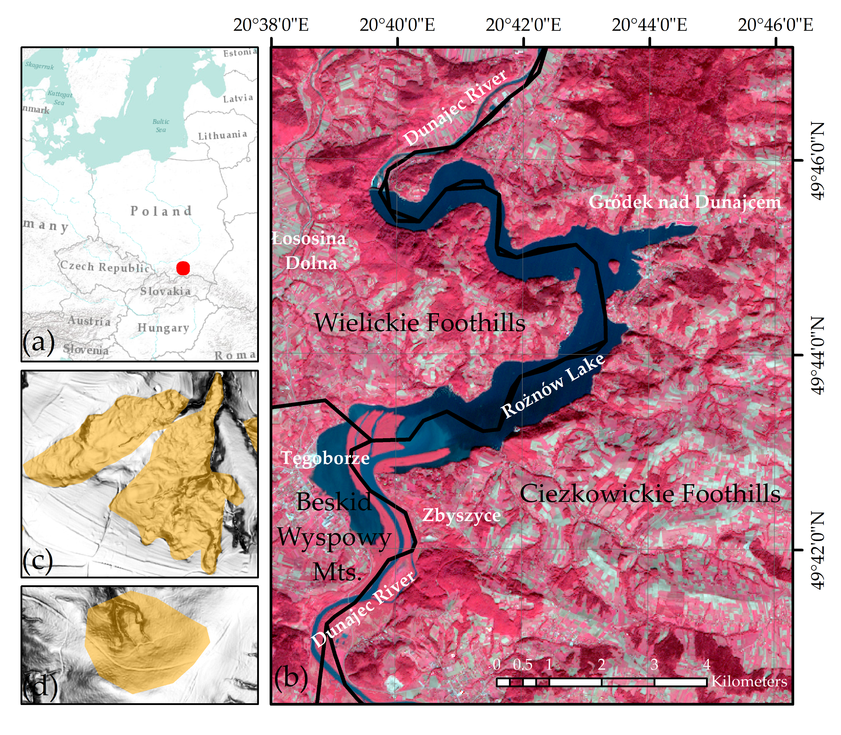
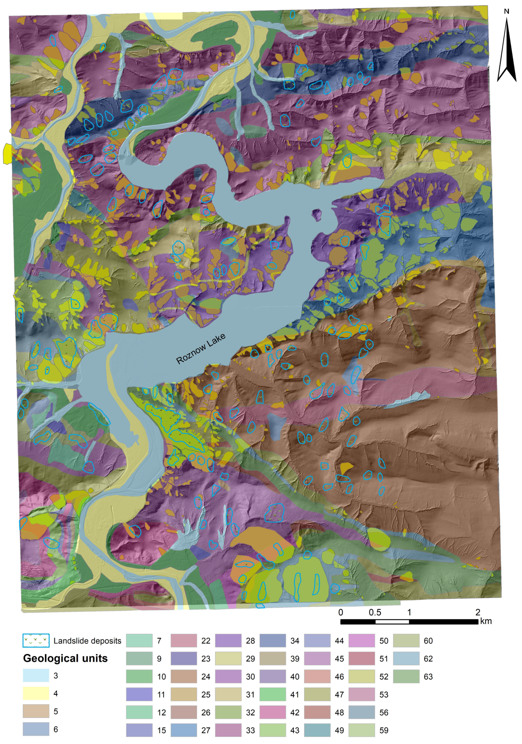
3.1. Study Area and Geological Conditions

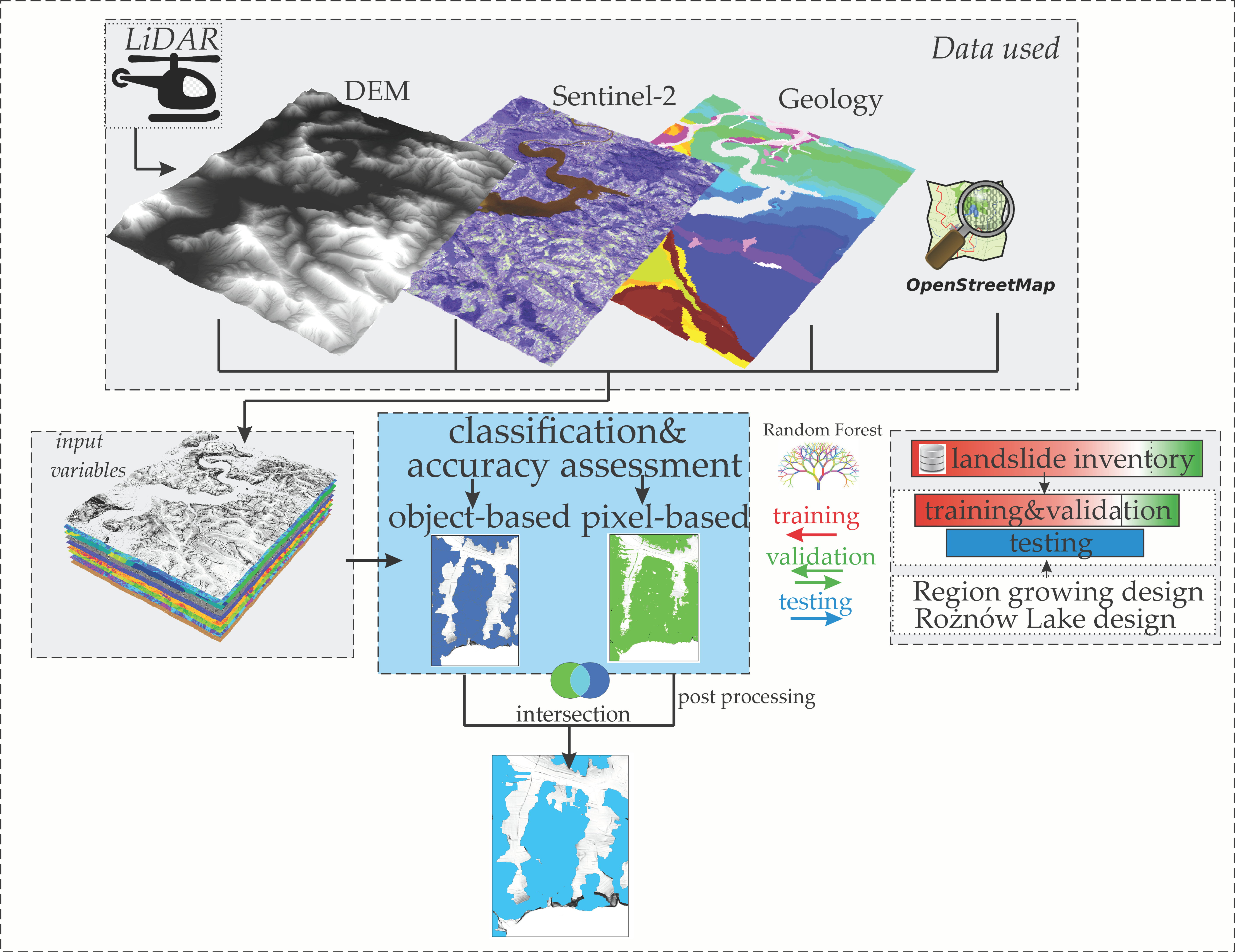
The study area is located in the vicinity of Rożnów Lake, in the central part of the Outer Carpathians, in the Małopolskie municipality, Poland (Figure 1). The study area covers from 49°40′N to 49°46′N latitude and from 20°38′E to 20°48′E longitude. Within the study area of 157 km², around 21 km² is affected by landslides. This means that landslides occupy 13% of the entire study area. Within the study area, there are translational, rotational, or combined rock-debris slides and typical debris slides [73,74,75,76]. Based on Vernes’ classification, updated by Hungr et al. [74], landslides within the study are slow- to very slow-moving landslides. The landslide activity is significantly connected with hydro-geological factors, such as rock stratification and precipitation. Activation of deep rockslides requires long continuous precipitation of 100 to 500 mm per month while cumulative rainfall of 50–400 mm over the course of 2–5 days can induce mudslides and debris slides [75]. Usually, north-facing landslides are found to be complex, while south-facing landslides tend to be insequent or subsequent [75]. Figure 1c,d presents the various landslide morphologies within the study area. Unfortunately, there are many landslides with smoothed morphology (Figure 1d), which makes them difficult to detect.

Appendix A Figure A1a presents the normalized difference vegetation index (NDVI), Corine Land Cover (CLC), and NDVI index (A-b) for the study area. According to CLC, the study area is mostly covered by non-irrigated arable land (26%), mixed forest (20%), and lands principally occupied by agriculture with significant natural vegetation (18%). The remaining parts are covered by various types of forest (coniferous forest, broad-leaved forest), plantations, pastures, and water bodies (8%). Appendix AFigure A1b presents the NDVI index calculated for Sentinel-2A data acquired at 25/03/2020. As can be observed, 53.7% and 31.8% of the whole area have values greater than 0.6 and 0.3, respectively. This indicates that most of the study area is covered by vegetation (forest and agricultural areas), which is in agreement with CLC.

The terrain of the Beskid Mountain Range area mainly has features of low- and medium-high mountains and medium-high foothills [77]. The slope length ranges from 0.6 to 1 km [75]. Predominant slope gradients are in the range of 0–68° and the relative elevations range from 266 to 613 m in the montane area. In sub-montane areas, slope gradients are in the range of 0–72° and 0–82° for Wielickie and Ciężkowickie Foothills, respectively. Correspondingly, the relative elevation within Wielickie and Ciężkowickie Foothills is from 232 to 486 m and 234 to 581 m, respectively. In Ciężkowickie Foothills, landslides range in size from 537 m² to 92 ha. In Wielickie Foothills, landslides range from 584 m² to 26 ha. In Beskid Mountains, landslides range from 925 m² to 37 ha. The mean size of the landslides within the study area is 3 ha. Large inactive landslides can be generally observed in Beskid Wyspowy in woodland areas, on upper slope segments, and in cones of depression [73]. The most susceptible area to land sliding is that directly adjacent to Rożnów Lake.

In Appendix B, the geological map for the study area, with explanation, is presented. The study site mainly comprises Eocene–Oligocene sandstones and shales and Upper Cretaceous sandstone and conglomerate–Lower Stebna layers. Additionally, many different geological subunits are interconnected with each other (see Appendix B). Based on Appendix B, it can be observed that the landslide bodies are mainly located in the boundaries/contacts of the units and steep slope areas along Rożnów Lake, where the slope stability is poor. These areas are mainly covered by sandstones and shales. For example, in the boundaries of the Eocene sandstone and shale in the Śląska series, Oligocene-aged shale of the Krosno layers is found in high slope areas along the lake and Paleocene–Eocene-aged spotted shale is found in the Magura Series. In contrast, landslides are less observed in medium-thick Oligocene sandstones and shales of the Śląska Series. Other geological units have a low susceptibility for landslides [73,75].

3.2. Data

Various data were utilized for this analysis. LiDAR data were acquired using a Riegl LiteMapper 6800i system based on the Q680i laser scanner. The point cloud planimetric density is equal to 4–6 points/m², and the estimated root mean square error for the height component is about 0.15 m [78]. The ability of LiDAR to capture topographic information is highly advantageous in forested areas [7,19,20]. The landslide inventory database (SOPO) from the Polish National Geological Institute was utilized to capture the training and testing datasets. The SOPO database consists of geological data, in addition to information on landslide locations and their type, and on areas prone to mass movements.

The location of existing landslides was collected in the SOPO database by the method approved by Polish National Geological Institute [79]. This method included conventional techniques, mostly comprising field reconnaissance, the visual interpretation of aerial photographs, the analysis of historical data, and detailed geomorphological/geological analysis [75]. Landslides within the study area stored in the SOPO database were mapped during field work in the years 2010, 2011, 2012, 2013, 2014, and 2015 [76,80,81]. Additional mapping work was also performed on the basis of topographic maps at a 1:10,000 scale supported by stereoscopic analyses of aerial photographs and LiDAR data [82]. In addition to LiDAR and landslide inventory maps, geological maps over the study area were acquired in raster format from the Polish National Geological Institute. Furthermore, Sentinel-2A images acquired on 25/03/2020 and road network maps from Open Street Map were utilized.

Table 1. Data used, their types, and their sources.

Data Used	Data Type	Source
DEM	Point cloud	LiDAR [78,83]
Landslide inventory map	Raster	http://geoportal.pgi.gov.pl/portal/page/portal/SOPO
Geology map	Raster	Polish National Geological Institute
Sentinel-2A	Raster	https://scihub.copernicus.eu/
Road network	Shapefile	Open Street Map

summarizes the data used, and their types and sources.

4. Methods

An overview of the methodology applied is presented in Figure 2. The 2-m DEM generated from the LiDAR point cloud was used for the extraction of topographic variables. Other data, such as Open Street Map (OSM) or Sentinel-2A data, were used for additional non-topographical layer extraction. Moreover, we utilized the DEM to extract the streams’ networks and Sentinel-2A to extract the extent of Rożnów Lake. A detailed description of the extracted variables is presented in Section 4.1. The extracted variables were used for supervised classification using pixel- (PBA) and object-based (OBIA) approaches. Despite the various classification approaches used, we classified the study area using the two training and testing strategies presented in Section 4.4. The accuracy parameters were computed for each classification approach and for the various training and testing strategies.

Additionally, taking advantage of various processing approaches (pixels vs. object), the final detection map was generated for overlapped results from PBA and OBIA. Then, additional refinement was carried out (see Section 4.6). Furthermore, by utilizing the RF algorithm, we were able to indirectly assess the feature relevance in automatic landslide mapping.

4.1. DEM Generation and Feature Extraction

The classified LiDAR point cloud was acquired within the IT System of the Country Protection (ISOK) project [78,83]. LiDAR point cloud filtration within this project was performed using different software, mainly TerraScan based on Axellson’s filtering method [84,85,86]. A filtered point cloud was corrected manually based on a visual inspection of the point cloud and aerial photographs. A classified LiDAR point cloud with a mean density of 4–6 /m² was used to generate the base DEM. The natural neighbor interpolation method was used to avoid smoothing of possible terrain breaklines represented in the original point cloud. However, according to the recommendations provided in [14], we resampled the base 0.5-m DEM into a 2-m resolution. This allowed us to preserve all landslide surface features while significantly decreasing the data volume and removing the artifacts present in the data at the original resolution. The issues connected with the suitable DEM resolution have been investigated by various scientists, many of whom reported that the finest DEM resolution is not the best choice [12,14,15,26,87]. Then, DEM derivatives (also called topographic variables or land-surface variables and DEM variables) were calculated from the DEM. Based on a literature review, the DEM variables presented in

Table 2. Variables used for landslide detection with the setting, software, and methods utilized to calculate them.

Variable	Kernel Size/Setting	Implementation	PBA (ArcGIS)	OBIA (eCognition)	Examples of Application
DEM-related variables
DEM	-	-	√	√	[7,12,13,14,15,19,20]
aspect	-	[97]	√	√	[12,19]
side exposure index (SEI)	-	[97]	√	√	[16]
flow direction	-	ArcGIS	√	√	[7,13]
roughness	7 × 7	[14,98]	√	√	[4,7,12,13]
slope	15 × 15	[97]	√	√	[7,12,13,19]
curvature	15 × 15	[97]	√	√	[7,12,13,27]
topographic position index (TPI)	15 × 15	[99]	√	√	[90]
openness	25 × 25 (interpolated DEM)	[14] ${\mathrm{DEM}}_{25\mathrm{m}}-{\mathrm{DEM}}_{2\mathrm{m}}$	√	√	[7,13]
hillshade	8 various sun angles	ArcGIS	√	√	[10,12,15,34,45]
compound topographic index (CTI)	-	[97]	√	√	[26,87,90]
elevation relief ration (ERR)	10 × 10	[87]	√	√	[87]
integral relief (IR)	10 × 10	[87]	√	√	[87]
integrated moisture index (IMI)	-	[97]	√	√
Other variables
geology	-	-	√	√	[90]
NDVI	-	(NIR − RED)/ (NIR + RED)	√	√	[12]
roads proximity	-	Euclidean distance buffering	√	√	[90]
streams proximity	-	Euclidean distance buffering	√	√	[7,12]
lake proximity	-	Euclidean distance buffering	√	√	-
Geometry variables
count	-	eCognition		√	-
compactness	-	eCognition		√	[13]
rectangularity	-	eCognition		√	-
shape index	-	eCognition		√	[10,13]
roundness	-	eCognition		√	-
asymmetry	-	eCognition		√	-
length/width	-	eCognition		√	[13]
border length	-	eCognition		√	-

were utilized. However, for OBIA, the mean pixels’ value of DEM variables inside the object was used. We applied 14 DEM variables, which are widely used and recommended in the literature [7,10,13,14,15,19,20,87]. Roughness, curvature, mean slope, topographic position index (TPI), and openness were calculated using various kernel sizes according to the recommendations provided by Pawluszek et al. [14]. To take advantage of the hillshade, which is calculated by illuminating the DEM with sunlight coming from a specific direction, we calculated the hillshade layers using eight sun angles (Figure 3) and then summed these layers into one hillshade layer. This allowed us to simulate the sunlight coming from various directions [34].

In contrast to PBA, OBIA takes advantage of various geometrical variables (compactness, rectangularity, etc.). These variables were applied in the OBIA approach. In addition to the topographical variables calculated from the DEM, the geology, normalized difference vegetation index (NDVI), and proximity to roads, lake, and streams were also implemented in the classification. A large amount of previous research [11,12] has utilized the NDVI for landslide identification. NDVI application is only effective in the detection of recent catastrophic events that generate explicit and visible land cover changes (before and after the event), including loss of vegetation, the presence of fresh soil, and the exposure of debris. Nevertheless, we also utilized NDVI as an additional layer for better segmentation and possible landslide boundary extraction. Landslide boundaries usually appear along various land use classes (rivers, streams, forest boundaries, etc.). Additionally, the NDVI layer was used for the Rożnów Lake extraction (NDVI < 0), which afterwards allowed for the extraction of the lake proximity variable.

Geology is one of the most important aspects that influences the occurrence of landslide identification and has been applied in many studies [30,88,89,90,91,92,93,94,95,96]. However, the proximity of roads and water reservoirs (lake/streams) are also reported as critical factors that influence landslide occurrence [89,90,91,92,94,95,96]. Information on the settings, methods, and software used are specified in Table 2, while the interrelationships of data used, and the extraction of various landslide classification variables are shown in Figure 3. Table 2 also provides the literature sources where particular variables are explained in detail.

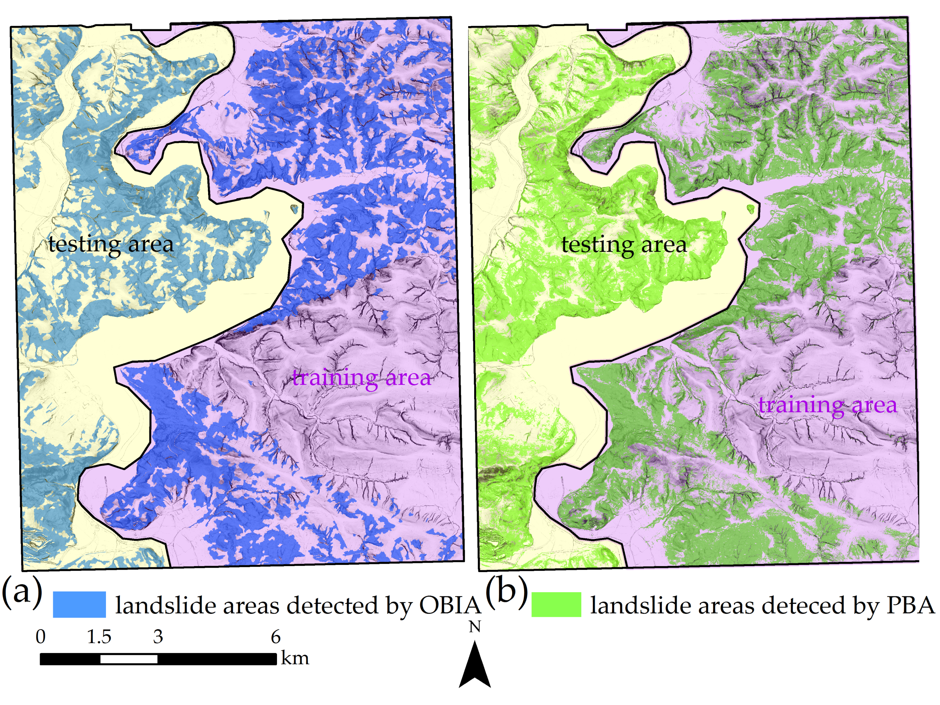
4.2. Pixel-Based and Object-Based Classification

An overview of the implemented PBA and OBIA classification is depicted in Figure 4. In the pixel-based approach, all used features are treated as a raster that is co-registered and resampled into the common resolution of 2 m. This makes a per-pixel analysis computationally effective [12]. As can be seen in Table 2, PBA, unlike OBIA, does not consider geometrical and contextual information [12,19,33,68]. In object-based classification, also known as geographic object-based image analysis (GEOBIA) or an object-oriented approach (OOA), the study area is segmented into groups of meaningful homogeneous objects [12,68]. This approach assumes that the neighboring pixels likely belong to the same class or object. A segmented object in OBIA can then be classified using spectral, geometric textural, or spatial variables and relationships. Based on [7,8,10,11,12,13,15,68], landslides are better represented by heterogeneous objects (collection of pixels) rather than single pixels. The first and the most important step in OBIA is the segmentation of the study area into objects that are candidates for landslides. Methods like multiresolution image segmentation and simple linear iterative clustering are predominantly used for the segmentation of objects. Some segmentation algorithms require scale parameters that influence the shapes and sizes of the resulting objects. These scale parameters vary depending on the applied segmentation algorithm. Moreover, the selection of appropriate scale parameters is not a straightforward task. In addition, landslides have a multiscale character. This means that in the real world, landslides come in a wide range of shapes and sizes, thus tuning segmentation scale is challenging. For this reason, various algorithms for scale tuning have been proposed in the literature (e.g., plateau objective function), which combined with expert knowledge allows for more effective landslide detection; however, the problem remains when landslides with significantly different sizes exist [11,28]. Because our research goal was to investigate the influence of the ratio between the training area and testing area, we utilized a trial-and-error procedure, which is also applied in the literature, to estimate the scale value [100]. We set each of the shape and compactness parameters equal to 0.5. This segmentation was performed for all extracted variables using multiresolution segmentation in eCognition.

4.3. Random Forest Classifier and Variable Importance

For the numerical investigations within this research, a mature ML classifier, random forest, was used in both approaches (PBA and OBIA). This is a nonparametric classifier developed by Breiman [101]. The RF classifier allows reliable classification results to be achieved using predictions derived from an ensemble of decision trees [101]. This is a crucial advantage that allows for a dimensionality reduction of the RS data. In the literature, this classifier is widely applied to various RS applications, such as land cover mapping [102,103] and landslide detection [12,19,20]. Detailed information on RF classification can be found in [101,104]. Moreover, this classifier can be effectively applied to select and rank variables with the greatest ability to discriminate between the target classes based on the impurity function of the Gini index, which is known as the mean decrease or Gini importance [101,104,105]. In Section 4.2, we provide an evaluation of the variable importance within PBA and OBIA classification. Additionally, a large feature set can cause problems, such as: (1) A long time needed to train the algorithm, (2) a long time and many resources needed to generate the variables, and (3) overfitting when too many irrelevant features are utilized [19]. Hence, the feature relevance assessment is a highly important aspect of the classification task. Nevertheless, we did not reduce our input variables because they did not decrease the classification time. However, if a larger study area is analyzed and more input layers are used, this variable reduction would be beneficial. During the training process, cross-validation was performed (Figure 4). This means that 10% of the training samples was removed from the training dataset and used to perform cross-validation. This allowed the evaluation of the accuracy of the predictive model applied and to fine tune this model. After the training process, formal classification was performed for the whole investigated area using various training and testing strategies, which are presented in the next subsection. The RF classification for both approaches (PBA/OBIA) was performed for 500 trees, with the tree depth equal to 30.

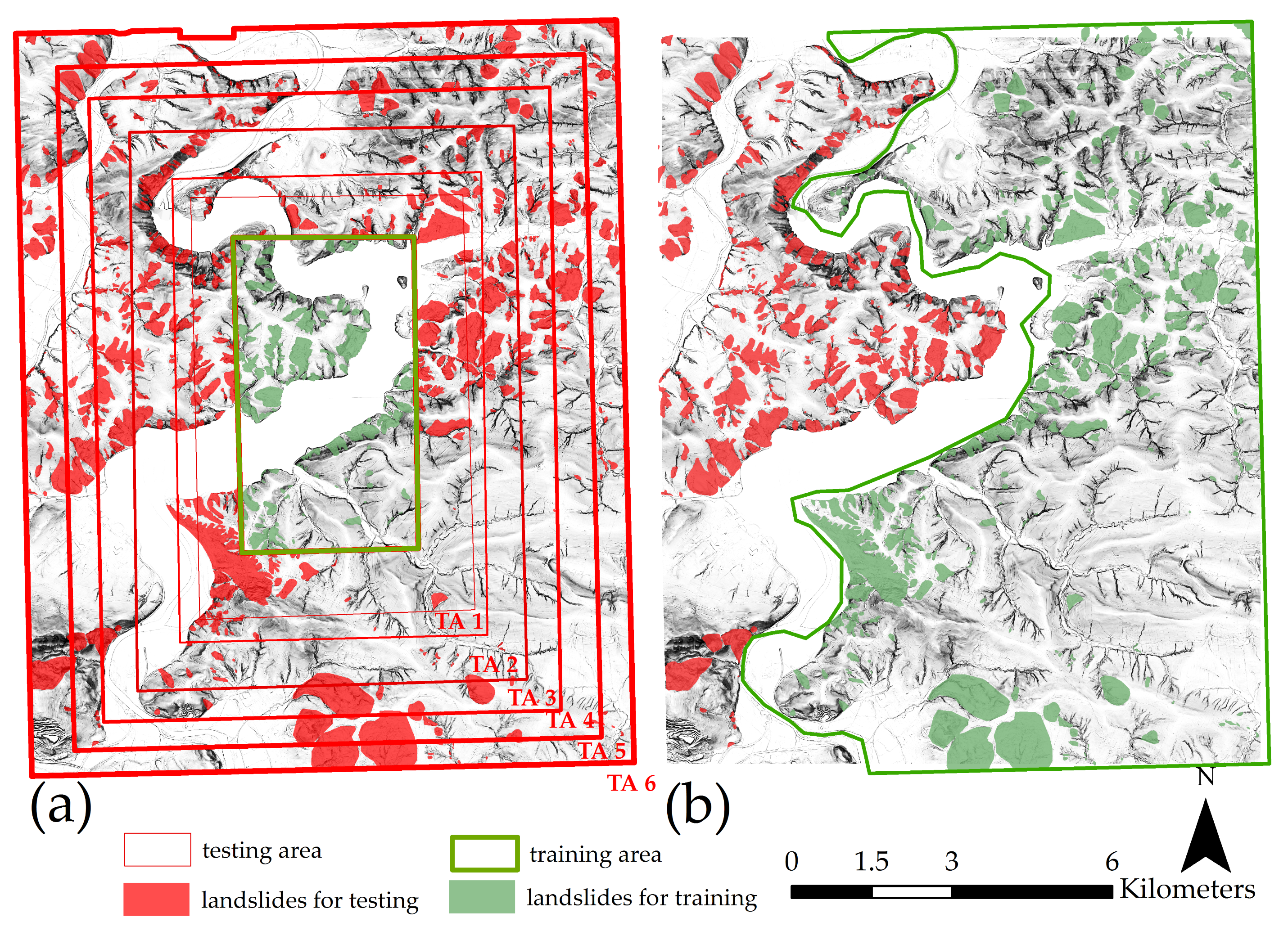
4.4. Training and Testing Strategies

Selection of the training samples is a critical step in supervised classification and the focal point of our study. According to [36,106], the training sample size has a larger impact on the classification accuracy than the algorithm itself. This conclusion was made based on an evaluation of the impact of training data size on various classifiers in land cover mapping. This issue is especially important in deep learning methods, where a large amount of well-labelled training samples is needed to prevent the classifier from overfitting [107]. Using various training sample sizes, Huang et al. [24] achieved an OA between 69% and 75%. However, OA is not the best estimator of the classification results, particularly for imbalanced classes. Nevertheless, this result shows that the training sample quantity influences the accuracy of the classification. Therefore, the acquisition of ground truth samples is a key factor when planning feature detection based on supervised classification methods. In addition to the quantity of training samples, the strategy for training sample selection is also important. Based on the literature, there are generally two sample selection strategies: manual and random sampling design [102,103,108]. Random sampling design is based on the identification and labeling of small random patches of homogeneous pixels/objects in an image [108]. Chen et al. [19] reported that random sampling design introduces the effect of spatial autocorrelation, which affects the classification accuracy. In manual sampling design, the study area is split into two datasets (training and testing) based on administrative or environmental boundaries. Training samples are spatially compact with no autocorrelation effect, unlike random sampling design. Manual sampling design is thus more reasonable from a practical point of view. Collecting landslide ground truth data is time-consuming. Consequently, these ground truths come from landslide inventory maps generated for specific regions. Landslide inventories are usually performed systematically on a part-by-part basis. Therefore, areas that have already been investigated and mapped can be used for training the algorithm and predicting landslide locations in areas where landslide inventory maps have not yet been generated (especially in poorly accessible areas).

We used a manual sampling design in our study and utilized landslide polygons and corresponding landslide pixels delivered from the SOPO inventory to train OBIA and PBA variants of classifiers, respectively. However, we implemented the training–testing split ratio (TTR) (compare Figure 4) according to two various strategies. In the first strategy, training samples were selected in the center of the investigated area and covered 13% of the entire study area. The remaining portion of the study area consisted of six testing areas (TAs), which were split using the region growing approach (Figure 5a). These six various TAs (

Table 3. Overview of the applied training sample size in the region growing testing design. TSQ—training samples quantity of the entire study area; TTR—training-testing split ratio; LTSQ—landslide training samples quantity of the entire classified area; and NLTSQ—non-landslide training samples quantity of the entire classified area.

Areas	No. Landslides	Domain [km2]	Landslide Areas [km2]	Non-Landslide Areas [km2]	TSQ [%]	TTR	LTSQ [%]	NLTSQ [%]
Training area	156	20	4.3	15.7	-
TA 1	149	20	5.4	14.6	50	1	10.7	39.3
TA 2	197	50	6.4	23.6	28.5	0.4	6.1	22.4
TA 3	335	56	9.8	46.2	26	0.35	5.6	20.4
TA 4	455	81	13.9	67.4	19.8	0.25	4.3	15.5
TA 5	563	106	17.2	88.8	15.9	0.19	3.4	12.5
TA 6	646	137	18.8	118.2	13	0.15	2.7	10.3

) were used for region growing testing. For instance, this means that the training quantity for TA 1 covers 50% of the total investigated area and for TA 6 covers 13% of the total investigated area (Figure 5a). This also corresponds to a training-split ratio of 1 and 0.15 for TA 1 and TA 2, respectively. In the second strategy (natural boundary splitting design), the study area was split into a testing and testing area along the boundary designated by Rożnów Lake and Dunajec River (Figure 5b). In this variant, the training area covers 54% of the entire study area. The quantitative values of the training samples in various testing strategies are presented in Table 3 and

Table 4. Overview of the used training sample size in the natural boundary splitting design. For the explanation of the abbreviations, see Table 3.

Area	No. Landslides	Total Area [km2]	Landslide Areas [km2]	Non-Landslide Area [km2]	TSQ [%]	TTR	LTSQ [%]	NLTSQ [%]
Training area	398	85	13.1	71.9	-
Testing area	404	72	8.3	63.7	54	1.2	8.3	45.7

for the region growing and the natural boundary splitting designs.

4.5. Classification Accuracy Parameters

To directly compare the accuracy of OBIA and PBA for various testing areas, we carried out an accuracy assessment at the pixel level. For this process, landslide shapefiles from the landslide inventory database were rasterized with a 2-m resolution and overlaid with the achieved PBA classification results. For OBIA, additional rasterization of the classification results was needed to overlay the OBIA results with the reference data acquired in the framework of the SOPO database. To compare the classification accuracy and evaluate the landslide detection skills of the tested variants, the confusion matrix for a particular variant was calculated. This matrix includes the true positive (TP), true negative (TN), false positive (FP), and false negative (FN) values. Based on these values, the overall accuracy (OA) of the model is calculated as follows:

$$\mathrm{OA}=\frac{\mathrm{TP}+\mathrm{TN}}{\mathrm{TP}+\mathrm{FP}+\mathrm{TN}+\mathrm{FN}}.$$

(1)

When comparing the classification results, we followed the recommendation in [103] to investigate more than just the OA. The F1 score, probability of detection (POD), and probability of false detection (POFD) are additional measures for the accuracy parameter:

$$\mathrm{F}1 \mathrm{Score}=\frac{2\times \mathrm{recall}\times \mathrm{precision}}{\mathrm{recall}+\mathrm{precision}}=\frac{2\times \mathrm{TP}}{2\times \mathrm{TP}+\mathrm{FP}+\mathrm{FN}},$$

(2)

$$\mathrm{POD} \left(\mathrm{recall}\right)=\frac{\mathrm{TP}}{\mathrm{TP}+\mathrm{FN}},$$

(3)

$$\mathrm{POFD} \left(\mathrm{fallout}\right)=\frac{\mathrm{FP}}{\mathrm{FP}+\mathrm{TN}}.$$

(4)

These parameters are especially important when imbalanced data are the subject of classification. POD provides a view of correctly classified landslide data, while POFD portrays how many non-landslide areas have been classified as landslides. The preferred value of the POD is 1, while that of POFD is zero. The F1 score defines the harmonic average of precision and recall. These additional accuracy assessment parameters are specifically important if the mapping focuses on small classes (i.e., classes of a limited extent in the image data). Small classes will have little influence on the OA, although they may be key in determining the usefulness of the classification [103]. This situation appears when dealing with landslide mapping. It is relatively rare for landslides to cover 50% of the whole study area; therefore, their influence on the OA is lower than that of the non-landslide class. For our study area, the landslide density is 14.7% of the whole study area (23.1 km² of landslide areas and 157 km² of non-landslide areas). Thus, the influence of the landslide class on the OA is small. It thus makes sense to also investigate the F1 score, POD, and POFD indexes to obtain a better overview of the classification accuracy and landslide detection skills.

4.6. Post-Processing and Final Landslide Map Generation

Because landslide extents detected by the OBIA approach are represented by multiple objects or multiple pixels, we performed a post-processing refinement of the results. We determined the most probable landslide extent by extracting the regions detected by PBA, as well as by OBIA. The intersection of both results provided the most likely results. Additionally, when observing the final results, we noticed many small and elongated objects that do not represent landslide areas. Since the minimum landslide size within our study area is equal to 537 m² (estimated based on SOPO inventory), we consequently removed objects smaller than 500 m² from the intersected results. A shape/perimeter index lower than 5 was another threshold parameter. Finally, filtering of the result using a median filter with a 6 × 6 window size was performed to fill the small holes within the landslide bodies.

5. Results

5.1. Accuracy Assessment of Various Training and Testing Strategies

The cross-validation rate achieved during RF training was higher than 0.98, which means that the models were correctly trained, and data could be classified using RF. As previously mentioned, in the region growing sample design, we performed classification of the total study area using training samples located in the center of the study area. Then, an evaluation of the results was performed for the growing testing areas.

Table 5. Accuracy assessment for training and testing strategy 1 (region growing testing). Testing areas 1–6 abbreviated as TA 1–6.

Testing Area	Method	TTR	F1 Score	POD	POFD	OA [%]
TA 1	PBA-RF	1	0.57	0.83	0.29	74
	OBIA-RF		0.58	0.88	0.31	73
TA 2	PBA-RF	0.4	0.53	0.85	0.31	72
	OBIA-RF		0.53	0.88	0.33	71
TA 3	PBA-RF	0.35	0.44	0.83	0.34	69
	OBIA-RF		0.46	0.87	0.34	69
TA 4	PBA-RF	0.25	0.42	0.80	0.34	68
	OBIA-RF		0.46	0.86	0.33	70
TA 5	PBA-RF	0.19	0.42	0.79	0.33	68
	OBIA-RF		0.45	0.85	0.32	70
TA 6	PBA-RF	0.15	0.40	0.78	0.33	68
	OBIA-RF		0.43	0.84	0.32	70

presents the accuracy assessment parameters (F1 score, POD, POFD, and OA) for particular testing areas. These results could be refined using post-processing to increase their accuracy. However, to directly compare PBA and OBIA and the influence of the TTR on the detection results, refinement was not performed at this stage. Analyzing the achieved results, we can notice that the F1 score of both approaches (PBA vs. OBIA) is comparable; however, OBIA performed slightly better (completeness and precision) (Figure 6). This can be especially observed for TA 3–6. Notably, the same algorithm and parameters were utilized in both classification approaches. The classification accuracy changes only under various training sample sizes. This important finding is shown in Table 5. The detection landslide skills decrease subsequently with a decrease in the contribution of training samples in the total study area. Notably, the OA does not change significantly, and the other accuracy parameters, such as the F1 score and POD, consequently decrease. This fact is more obviously presented in Figure 6 for the F1 score accuracy measure. The region growing testing shows that the landslide detection skills decrease proportionally to decreases in the TTR. However, a substantial decrease is observed when the training sample quantity decreases from 50% to 26%. After this, we can observe a small decrease in accuracy. This proves the previously discussed issue when the OA index is used alone to evaluate landslide detection accuracy.

Based on the achieved results, it can be concluded that the best result was achieved with 50% of the training samples (F1 Score = 0.58). These results are limited, likely due to the imbalance in landslide and non-landslides classes. In the tested scenario, only 10% were landslide areas, while 40% were non-landslide areas.

To verify if accuracy above 70% and an F1 score at the level of 0.5 can truly be achieved when the training and testing areas are similarly large, we performed training and testing according to the natural boundary splitting design. The study area was split along the natural Rożnów Lake and Dunajec River boundary. Although, in this variant, the testing and training areas were similarly large (TTR = 1.2), we achieved slightly worse results. For instance, the OBIA approach provided an OA, F1 score, POD, and POFD equal to 72%, 0.48, 0.87, and 0.30, respectively (for comparison, for TTR = 1, the OA, F1 score, POD, and POFD were equal to 73%, 0.58, 0.88, and 0.31, respectively, in the region growing strategy).

Table 6. Accuracy assessment for training and testing strategy 2 (Rożnów Lake splitting).

Testing Area	ML Method	F1 Score	POD	PODF	Accuracy [%]
Łososina-testing area	PBA-RF	0.46	0.86	0.33	70
	OBIA-RF	0.48	0.87	0.30	72

presents the accuracy parameters for both classification approaches, while Figure 7 shows a graphical representation of the classification results.

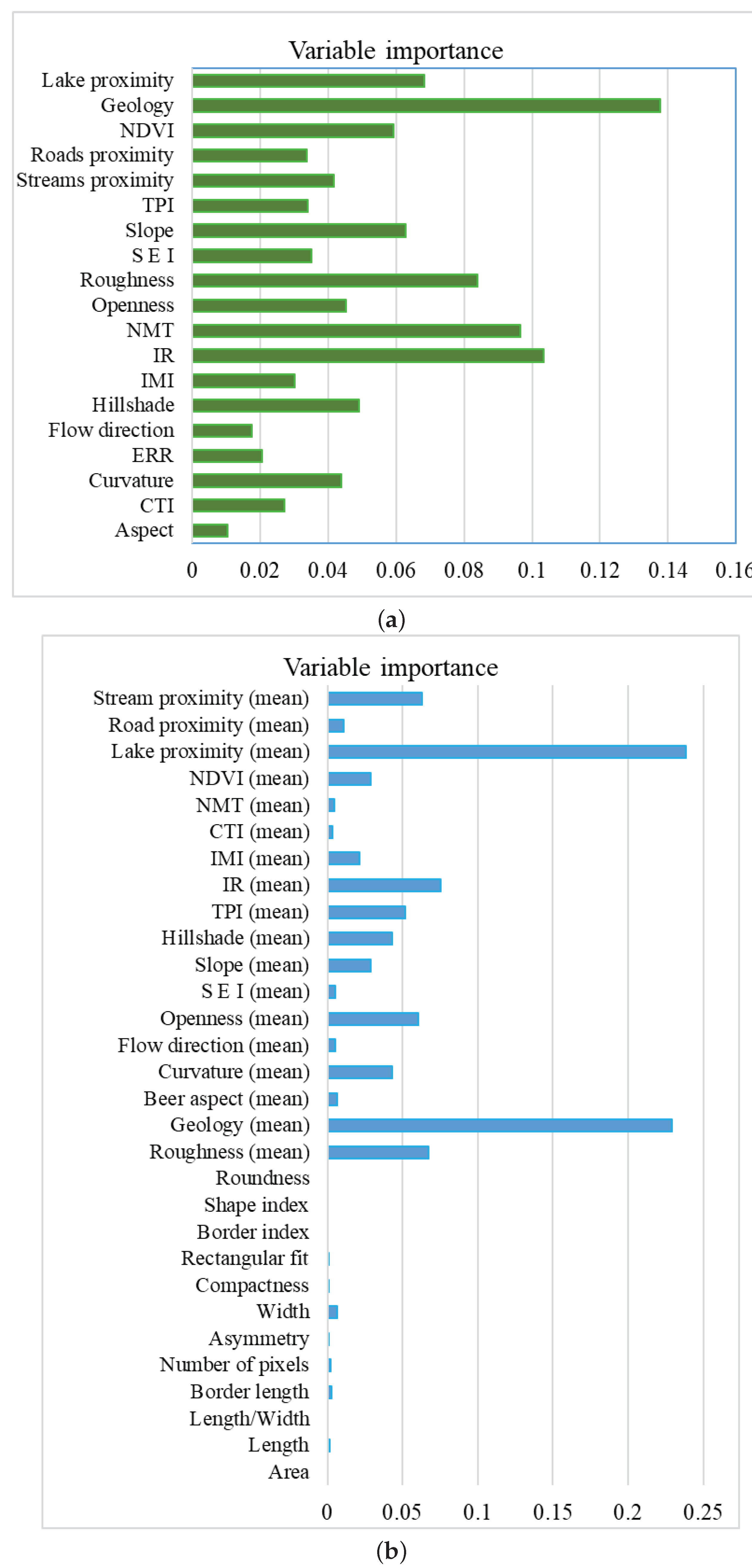
5.2. Feature Relevance

The feature relevance for classification can be assessed as an output from the RF algorithm training according to the Gini impurity reduction [101]. Figure 8 presents the variable importance for both classification approaches. As can be observed in both the PBA and OBIA classification approaches, the geology, DEM, and roughness are the most important variables. The geometric variables were found to be relatively unimportant in landslide detection using OBIA. The reason for this could be the segmentation settings, which lead to objects that did not result in significant geometric values. In this scenario, over-segmentation results in many small objects that represent the extent of one landslide body. Thus, the geometric parameters of segmented objects do not correspond directly to the landslide extent and therefore landslide object geometric parameters. Thus, to extract the boundary of one landslide body, several segmented objects of this landslide should be merged together.

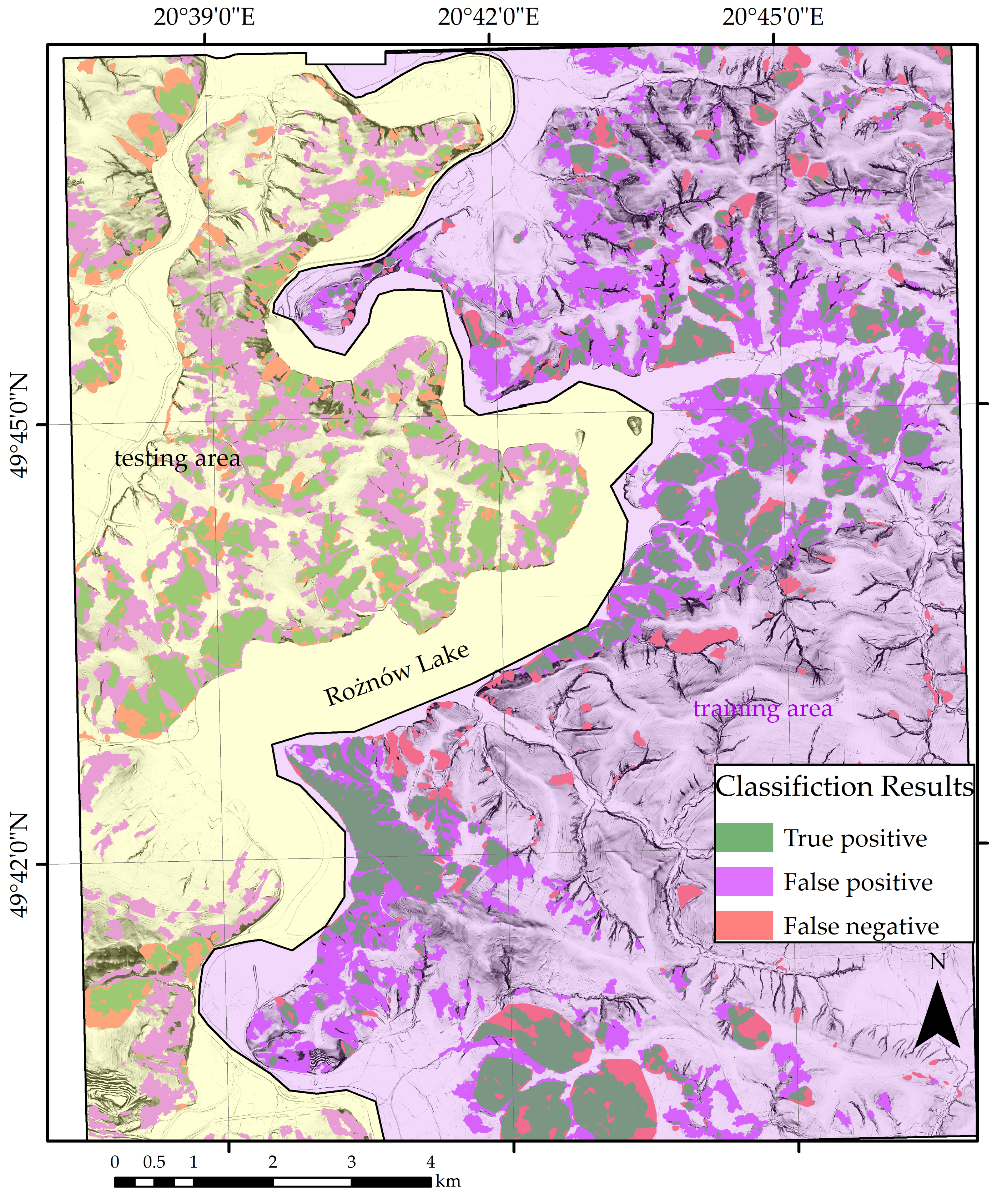
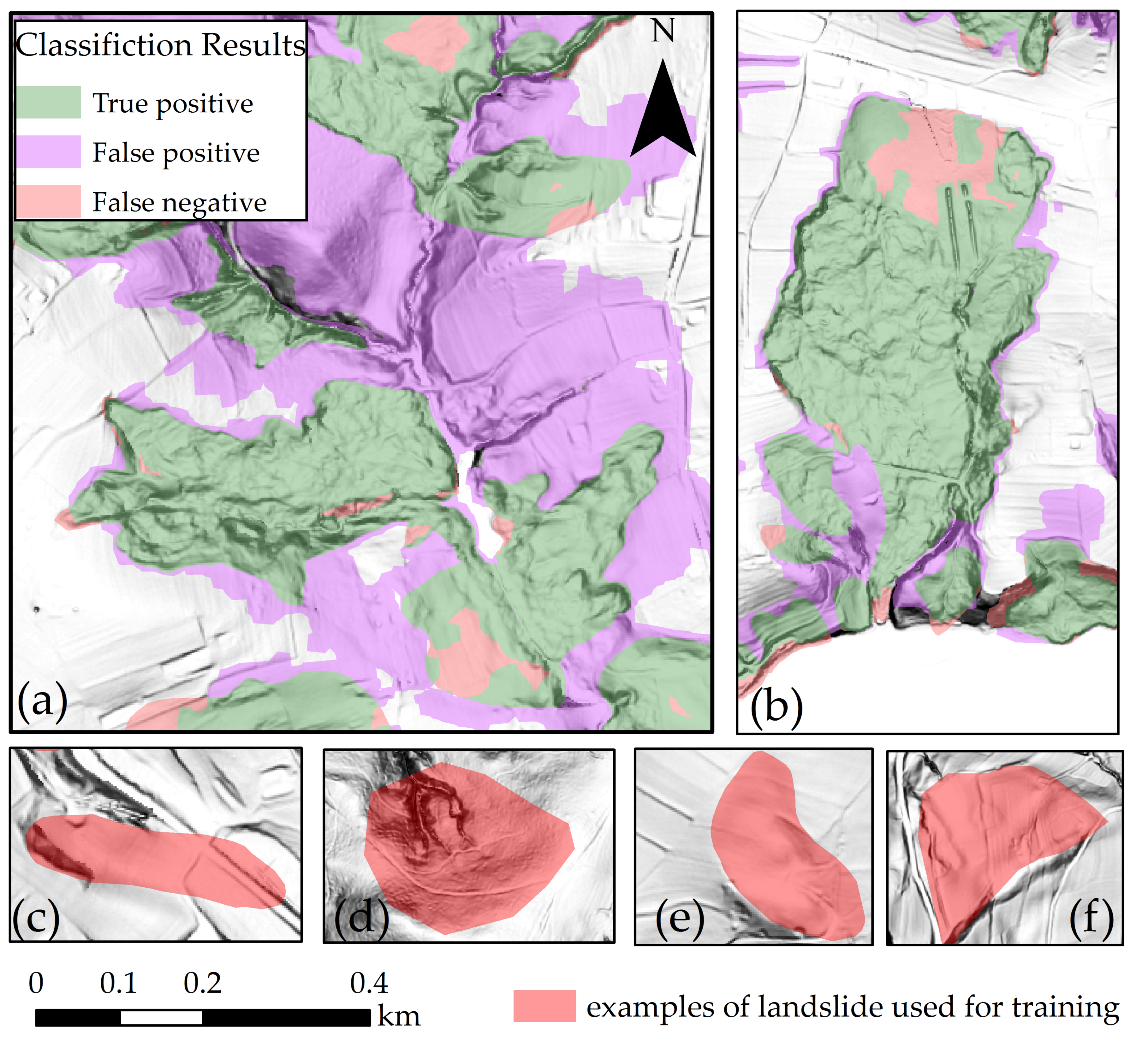
5.3. Final Landside Map Generation

The common elements of the OBIA and PBA results from the second strategy (natural boundary splitting design) were then refined. This refinement was performed via the post-processing step described in Section 4.6. The final map of the detected landslides with TP, TN, and FN is presented in Figure 9. The accuracy indexes after the subsequent post-processing steps are presented in

Table 7. Accuracy assessment for training and testing strategy 2 with the accuracies acquired after post processing steps (Rożnów Lake splitting).

Classification Results	Post-Processing Step	F1 Score	POD	POFD	OA [%]
PBA-RF	-	0.46	0.86	0.33	70
OBIA-RF	-	0.48	0.87	0.30	72
PBA&OBIA	intersection of PBA and OBIA	0.48	0.73	0.23	76
PBA&OBIA refinement 1	small elongated objects removed	0.50	0.62	0.15	81
PBA&OBIA refinement 2	median filtering	0.50	0.71	0.19	80

. Based on these, we can observe that the intersection of the PBA and OBIA approach, in addition to the removal of small and elongated objects, helped to decrease the POFD index. This means the minimization of over-classification or over-mapping (a high false positive rate). Medial filtering slightly increased POFD but also increased POD, which is desirable. From another point of view, these post-processing steps also decreased the POD, which reflects the probability of correctly detected landslides. However, the OA and F1 scores subsequently increased in the following post-processing steps. Increasing the F1 score indicates the performance of classification by taking into account true positives (correctly classified landslides), as well as false positives (wrongly detected landslides).

6. Discussion

6.1. Landslide Classification Accuracy with Respect to the Training Samples

Based on the results presented in Section 4.1, it can be observed that the F1 score and OA with respect to the TTR decreases proportionally to the decreased training sample contributions in the whole investigated study area. However, when comparing the OBIA and PBA results, OBIA performed better for testing areas 3–6 when the TTR decreased. Thus, it can be concluded that OBIA performs better than PBA when the quantity of training samples is smaller. Additionally, based on the region growing testing design, it can be assessed that to achieve an F1 score at the level of 0.5, the training area should be as large as the testing area. Therefore, this should be considered when performing landslide detection using supervised classification.

Additionally, when comparing the results from the region growing design and natural neighbor splitting design, it can be seen that the landslide detection skills are smaller in the second strategy. The term “landslide detection skills” refers to how well the algorithm detected both classes: landslide and non-landslide areas. This can be represented by the F1 score. Comparing results from the first and second strategy where a TTR around 1 (training and testing area are similarly large) was applied, higher landslide detection skills of the second strategy should be expected. The explanation for this could be a smaller landslide class or landslide sample contribution in the training samples. In the region growing design for similarly large areas for training and testing, landslide samples covered an area of 10.7 km², while in the natural splitting design, they covered 8.3 km². Another issue could be related to the landslide morphology, because in both strategies, various landslides were used for classification. The terrain roughness, value of curvature, and other variables can differ between landslides.

Furthermore, study area conditions could be the reason for slightly smaller landslide detection skills in the second strategy. These could be geological changes, various elements of landslide training samples due to the many types of land used (agricultural vs. forests), etc. Specifically, this relates to how the classification accuracy changes under various geological and environmental conditions, also taking into account the local morphometry of a particular landslide (e.g., training the algorithm on a study area in a hilly or mountainous terrain covered by forest and evaluating it using a study area that is extensively cultivated, and vice versa). In addition to this aspect, the training sample number and training sample size are also noteworthy aspects to investigate. In this research, we investigated the training–testing split ratio. However, the training sample number can also influence the classification results. Thus, the topic of selecting training samples is not exhausted and various aspects were not covered in this paper but should be investigated in future works.

It is worth mentioning that the achieved accuracy of landslide detection from the natural splitting design is affected by the different characteristics of the training and testing areas. More specifically, landslides located on the one side of Rożnów Lake (training area) can have other characteristics than this located on the other side of the lake (testing area). In a perfect scenario, landslides used, or the training, that are randomly and evenly distributed across the investigated study can better capture a variety of the characteristics and can more effectively detect landslides. However, as was mentioned before, the collection of ground truth data across the study area is very challenging and time-consuming from a practical point of view. Usually, such ground truth data (landslide inventory) is generated on the part by part basis. In Poland, landslide inventory is performed commune after commune. In the case of the study area, Rożnów Lake and Dunajec River are also the border between two communes, namely Łososina Dolna commune (testing area) and Gródek nad Dunajcem (training area). Landslide inventory for Łososina was created in 2011 while for Dunajec around 2015. Thus, from the practical point of view, it is desirable to utilize existing landslide inventory for training and detecting landslides in the area where such an inventory is not available.

6.2. Comparison with Other Related Studies

Our final results for landslide automatic detection were achieved via integration of the PBA and OBIA results and the post processing refinement described in Section 4.6. Considering the classification accuracy measures (Section 4.5), we achieved moderate agreement with the ground truth data (F1 score = 0.5). Thus, there is still space for improvement in automatic landslide mapping. In addition to various data, approaches, and classification accuracy measures, we attempted to compare our results to those of other studies related to landslide detection based on DEM. However, it should be mentioned that direct comparison is not possible due to the various study areas used in various works or also different accuracy measures. Anyway, to somehow relate our study with some existing in the literature and to summarize our achievement and limitations, we made this comparison. To compare these results with those in [13] and those in our previous studies [14,15], we additionally calculated the Kappa index, which is also a frequently used classification accuracy measure in the RS community. Some scientists discussed the limitation connected with the Kappa index in accuracy evaluation [109,110]. Since some papers present Kappa and OA and/or recall only [13,14,15], we decided to not omit the Kappa index due to the limited number of presented accuracy measures, which can be used for comparison.

Comparing the accuracy measures of the other studies presented in

Table 8. Comparison with other works and accuracy assessment indexes.

Authors	Method	Study Area	F1 Score	POD (Recall)	POFD (Fallout)	K	Accuracy (OA)
	Presented research	Łososina, Poland	0.50	0.71	0.19	0.4	0.80
[12]	Deep learning	Oregon, USA	0.56	0.72	0.13	-	0.85
[12]	RF-PBA	Oregon, USA	0.51	0.66	0.14	-	0.83
[12]	ANN-OBIA	Oregon, USA	0.55	0.48	0.06		0.86
[13]	SVM-OBIA	Oberpullendorf, Austria	-	0.69	-	0.48	-
[17]	SICCM	Dixie Mountain	-	0.39	-	-	0.74
[17]	SICCM	Gales Creek	-	0.43	-	-	0.85
[17]	SICCM	Big Elk Creek	-	0.65	-	-	0.73
[19]	RF-PBA	Three Gorges, China	-	0.65			0.64
[20]	RF-OBIA	Three Gorges, China	-	0.71	-	-	0.77
[15]	SVM-OBIA	Łososina, Poland	-	0.71	-	0.6	0.85
[14]	SVM-PBA	Łososina, Poland	-	0.65	-	0.55	0.81

, the results achieved in this study are consistent with those of previous studies using similar methods [12,14,15,19,20], especially ML-based or deep learning classification methods [12] (compare Table 8). Nevertheless, these accuracy indexes still show only moderate landslide detection skills. The authors in [12] achieved a smaller POFD, which indicates a smaller amount of false positives when using similar OBIA and ML classification approaches. This is probably due to the specificity of the study area (Oregon, USA). From Google Earth satellite images, it is apparent that the majority of Oregon is covered by dense forest. There is only one city (Elkton), one main road (No. 38), and a lack of agricultural areas. Thus, the explanation for the higher false positive rate could be the forest coverage, which maintains the characteristic landslide topography. Additionally, when comparing our results with the work in [20] conducted on the Three Georges in China, similar results were obtained. When comparing OA with the work of [17], it can be stated that a similar accuracy was achieved; however, the POD (recall) presented in [17] was significantly smaller, especially for the study area of Dixie Mountain. Based on the results in Table 8, landslide detection in Dixie Mountain was the worst. This proved again that accuracy measures other than OA are needed (e.g., F1 score, POD, POFD, K) to reliably compare classification results between various areas with different landslide densities and different conditions. Additionally, the authors in [17] observed that the scarp identification and contour connection method (SICCM) mapped various study areas differently, either under-mapping or over-mapping in various study areas. Thus, there is no clear indication that SICCM mapped one study area better than another.

Based on the Kappa and POD, slightly better results were provided by Knevels [13]. The reason for the higher Kappa value could be the methodology applied in this study. Specifically, landslide detection in the area of Oberpullendorf in Austria was performed by OBIA and support vector machine (SVM) classification, but the authors in [13] integrated geomorphological mapping with the OBIA approach. Specifically, the authors focused first on landslide scarp detection and then on the detection of neighboring landslide bodies. The relationships between these features likely increase the algorithm’s detection skills. This strategy would be beneficial for landslide detection but is computationally more demanding and needs additional parameters to be tuned.

Additionally, by comparing the accuracy measures with the works of Pawluszek et al. [14,15], it can be concluded that previous approaches offer better detection skills. However, Pawluszek et al. [14,15] utilized a significantly smaller study area (26.3 km² compared to the 157 km² analyzed in this paper). An additional issue is the training sample designs that they utilized in their previous investigations. In [14], they utilized stratified random sampling to train the algorithm, while in [15], the authors manually selected random samples across the image. The authors of [19,111] also reported that random samples taken across an area affected by landslides are more beneficial for landslide detection rather than small coherent clusters used as training samples. However, this is the effect of a spatial auto-correlation, which contributed to the final accuracy of landslide detection. There is no clear indication whether this is an advantage or drawback of these specific training sample designs. Nevertheless, from a practical point of view, when the landslide ground truth data need to be collected during field investigations, a manual sample design is more pragmatic than a random sampling design. This is mostly due to the time needed to collect samples across the investigated area during field work. Therefore, based on the observations of our current and previous studies, the selection of the training samples is a significant aspect that influences the final results and should be undeniably considered when planning ground truth data collection during field work.

6.3. Opportunities and Limitations of the Presented Approach

A detailed analysis of the final landslide detection map reveals some opportunities and limitations of the proposed approach. A section of the landslide detection map is presented in Figure 10a,b as an example of these limitations and opportunities. For a better understanding of the classification performance, the classification results were superimposed on the hillshade map (Figure 10a,b). We selected these specific parts of the map to discuss various issues affecting landslide detection. In Figure 10a, the presence of many false positive results can be observed. This means that the landslides were over-mapped. In Figure 10b, we can observe very appropriate landslide mapping in the middle part of the landslide in the areas with clear and fresh topographical characteristics (rough surface, etc.). In the upper part of the landslide (Figure 10b), we can observe false negatives, which means that this area was not properly mapped by the algorithm as a landslide but rather as a non-landslide area. This is due to the smoothed morphology, which is changed by agricultural treatments. However, in the lower part of the landslide, where the topography is again smoother, we can observe significantly more false positives, similar to the situation in Figure 10a. To explain this issue, we investigated our training samples used for training the RF algorithm.

Figure 10c–f presents the landslides located in the training area in the second classification strategy. These landslides were mapped by geologists in the field and are included in the official national landslide database. The morphology of the landslides used for training (Figure 10c–f) clearly suggests that the characteristic landslide features were smoothed and altered. The reasons for this are probably denudation and/or agricultural treatments. In such cases, it is highly challenging to evaluate if a false positive is truly a false positive or if it is also a landslide body where the typical landslide morphology has been smoothed. Based on visual interpretation, some areas with rough terrain have been correctly classified by the algorithm and clearly show the landslide extent (green color). Additionally, here we can observe the problem of landslide feature visibility, which makes OBIA integration with geomorphological mapping (division into some characteristic landslide parts) more challenging or impossible. The problems are mostly connected with an appropriate landslide scarp definition, because in Figure 10c–f, these characteristic landslide features are invisible. Having considered these aspects, it is our opinion that to minimize landslide over-mapping (reflected by a high POFD index), altered and smoothed landslides should be removed from the training process. This will probably help in more effective landslide boundary extraction and will minimize the false positive rate. Additionally, another aspect is related to the quality of the reference data because the delineation of landslide polygons can be too sparse and generalized. This would influence the accuracy of landslide detection [106,112]. Therefore, the quality of landslide shapefiles located within the training site should be investigated and discussed in future works.

7. Conclusions

Training samples are essential for supervised classification. In the case of automatic landslide mapping, it is especially important to determine how much representative data is required to achieve the specified level of accuracy in landslide detection based on supervised classification methods.

The region growing testing performed in this study shows that landslide detection skills decrease proportionally to a ratio decrease of the training–testing area. However, a substantial decrease is observed when the training sample quantity decreases from 50% to 26%. The application of region growing testing allowed us to assume that the training areas should be as large as the testing area. To verify this assumption, training sample selection according to the natural splitting design, which covers almost half of the entire study area, was used as the second strategy. In this strategy, the OA and F1 score were 72% and 0.42, respectively, and proved our assumption that the appropriate ratio of the training–testing area would be around 1. Slightly lower landslide detection skills when compared to the region growing design (an OA and F1 score of 73% and 0.58, respectively) can be related to other aspects of training sample selection (training sample number, quality of landslide inventory, etc.) or the environmental condition of the study area, which should also be investigated in future works.

In addition to, the training–testing ratio, which was the main focus of this study, the final landslide detection map was also generated by the intersection of the OBIA and PBA approaches and refinement of the results. Refinement included median filtering and the removal of small elongated objects, which allowed us to remove false positives from the final results. However, we inferred that the smoothed and vanished morphology of the landslides used for training and/or the quality of the landslide inventory have a direct influence on the rate of false positives. Nevertheless, the achieved results (OA = 80% and F1 score = 0.5) are consistent with those presented in the literature.

The RF algorithm also allowed us to identify the most relevant variables for landslide detection. In both cases (PBA and OBIA), the geology and terrain roughness were the most important variables and should undeniably be used in landslide detection. Furthermore, geometry-related variables were insignificant in the OBIA approach, probably due to the undersegmentation strategy used for the OBIA classification in this study.

In summary, this study, supported by the comprehensive literature review, allows us to draw a few conclusions for further research on landslide detection approaches. Firstly, from a practical point of view, manual sampling design should be selected to evaluate the landslide detection skills of algorithms based on supervised classifications. Secondly, the OA measure alone should not be used to evaluate the classification results, especially for imbalanced classes. Further, the train–test ratio should be around 1 (the training area should be as large as the testing area). The quality of the landslide ground truth sample is also an important issue. Additionally, the removal of old and denudated landslides whose characteristic topography is not visible in the terrain’s morphology should be removed from the training samples. Moreover, the environmental conditions of various study areas and the influence of landslide detection skills should be tested in the future to assess the transferability of the algorithms. Finally, the landslide phenomenon, due to its complexity, is highly challenging to detect; thus, the integration of the OBIA approach with geomorphological mapping, also taking into account morphometry, would be preferable.

References

1. Dou, J.; Chang, K.T.; Chen, S.; Yunus, A.P.; Liu, J.K.; Xia, H.; Zhu, Z. Automatic case-based reasoning approach for landslide detection: Integration of object-oriented image analysis and a genetic algorithm. Remote Sens. 2015, 7, 4318–4342. [Google Scholar] [CrossRef] [Green Version]
2. Dramis, F.; Guida, D.; Cestari, A. Chapter three–nature and aims of geomorphological mapping. In Developments in Earth Surface Processes; Elsevier: Amsterdam, The Netherlands, 2011; Volume 15, pp. 39–73. [Google Scholar]
3. Tien Bui, D.; Shahabi, H.; Shirzadi, A.; Chapi, K.; Alizadeh, M.; Chen, W.; Tian, Y. Landslide detection and susceptibility mapping by airsar data using support vector machine and index of entropy models in cameron highlands, Malaysia. Remote Sens. 2018, 10, 1527. [Google Scholar] [CrossRef] [Green Version]
4. McKean, J.; Roering, J. Objective landslide detection and surface morphology mapping using high-resolution airborne laser altimetry. Geomorphology 2004, 57, 331–351. [Google Scholar] [CrossRef]
5. Booth, A.M.; Roering, J.J.; Perron, J.T. Automated landslide mapping using spectral analysis and high-resolution topographic data: Puget Sound lowlands, Washington, and Portland Hills, Oregon. Geomorphology 2009, 109, 132–147. [Google Scholar] [CrossRef]
6. Saba, S.B.; van der Meijde, M.; van der Werff, H. Spatiotemporal landslide detection for the 2005 Kashmir earthquake region. Geomorphology 2010, 124, 17–25. [Google Scholar] [CrossRef]
7. Van Den Eeckhaut, M.; Kerle, N.; Poesen, J.; Hervás, J. Object-oriented identification of forested landslides with derivatives of single pulse LiDAR data. Geomorphology 2012, 173, 30–42. [Google Scholar] [CrossRef]
8. Lu, P.; Stumpf, A.; Kerle, N.; Casagli, N. Object-oriented change detection for landslide rapid mapping. IEEE Geosci. Remote Sens. Lett. 2011, 8, 701–705. [Google Scholar] [CrossRef]
9. Wojciechowski, T.; Borkowski, A.; Perski, Z.; Wójcik, A. Airborne laser scanning data in landslide studies at the example of the Zbyszyce landslide (Outer Carpathians). Przegląd Geol. 2012, 60, 95–102. (In Polish) [Google Scholar]
10. Stumpf, A.; Kerle, N. Object-oriented mapping of landslides using Random Forests. Remote Sens. Environ. 2011, 115, 2564–2577. [Google Scholar] [CrossRef]
11. Martha, T.R.; Kerle, N.; van Westen, C.J.; Jetten, V.; Kumar, K.V. Segment optimization and data-driven thresholding for knowledge-based landslide detection by object-based image analysis. IEEE Trans. Geosci. Remote Sens. 2011, 49, 4928–4943. [Google Scholar] [CrossRef]
12. Prakash, N.; Manconi, A.; Loew, S. Mapping landslides on EO data: Performance of deep learning models vs. traditional machine learning models. Remote Sens. 2020, 12, 346. [Google Scholar] [CrossRef] [Green Version]
13. Knevels, R.; Petschko, H.; Leopold, P.; Brenning, A. Geographic Object-Based Image Analysis for Automated Landslide Detection Using Open Source GIS Software. ISPRS Int. J. Geo-Inf. 2019, 8, 551. [Google Scholar] [CrossRef] [Green Version]
14. Pawluszek, K.; Borkowski, A.; Tarolli, P. Sensitivity analysis of automatic landslide mapping: Numerical experiments towards the best solution. Landslides 2018, 15, 1851–1865. [Google Scholar] [CrossRef] [Green Version]
15. Pawłuszek, K.; Marczak, S.; Borkowski, A.; Tarolli, P. Multi-Aspect Analysis of Object-Oriented Landslide Detection Based on an Extended Set of LiDAR-Derived Terrain Features. ISPRS Int. J. Geo-Inf. 2019, 8, 321. [Google Scholar] [CrossRef] [Green Version]
16. Pawłuszek, K.; Borkowski, A.; Tarolli, P. Towards the optimal pixel size of DEM for automatic mapping of landslide areas. Int. Arch. Photogramm. Remote Sens. Spat. Inf. Sci. 2017, 42, 83–90. [Google Scholar] [CrossRef] [Green Version]
17. Bunn, M.D.; Leshchinsky, B.A.; Olsen, M.J.; Booth, A. A simplified, object-based framework for efficient landslide inventorying using LIDAR digital elevation model derivatives. Remote Sens. 2019, 11, 303. [Google Scholar] [CrossRef] [Green Version]
18. Leshchinsky, B.A.; Olsen, M.J.; Tanyu, B.F. Contour Connection Method for automated identification and classification of landslide deposits. Comput. Geosci. 2015, 74, 27–38. [Google Scholar] [CrossRef]
19. Chen, W.; Li, X.; Wang, Y.; Chen, G.; Liu, S. Forested landslide detection using LiDAR data and the random forest algorithm: A case study of the Three Gorges, China. Remote Sens. Environ. 2014, 152, 291–301. [Google Scholar] [CrossRef]
20. Li, X.; Cheng, X.; Chen, W.; Chen, G.; Liu, S. Identification of forested landslides using LiDAR data, object-based image analysis, and machine learning algorithms. Remote Sens. 2015, 7, 9705–9726. [Google Scholar] [CrossRef] [Green Version]
21. Cheng, G.; Guo, L.; Zhao, T.; Han, J.; Li, H.; Fang, J. Automatic landslide detection from remote-sensing imagery using a scene classification method based on BoVW and pLSA. Int. J. Remote Sens. 2013, 34, 45–59. [Google Scholar] [CrossRef]
22. Mezaal, M.R.; Pradhan, B.; Rizeei, H.M. Improving Landslide Detection from Airborne Laser Scanning Data Using Optimized Dempster–Shafer. Remote Sens. 2018, 10, 1029. [Google Scholar] [CrossRef] [Green Version]
23. Mezaal, M.R.; Pradhan, B.; Sameen, M.I.; Mohd Shafri, H.Z.; Yusoff, Z.M. Optimized neural architecture for automatic landslide detection from high-resolution airborne laser scanning. Appl. Sci. 2017, 7, 730. [Google Scholar] [CrossRef] [Green Version]
24. Sameen, M.I.; Pradhan, B. Landslide detection using residual networks and the fusion of spectral and topographic information. IEEE Access 2019, 7, 114363–114373. [Google Scholar] [CrossRef]
25. Pradhan, B.; Mezaal, M.R. Data mining-aided automatic landslide detection using airborne laser scanning data in densely forested tropical areas. Korean J. Remote Sens. 2018, 34, 45–74. [Google Scholar]
26. Sîrbu, F.; Drăguț, L.; Oguchi, T.; Hayakawa, Y.; Micu, M. Scaling land-surface variables for landslide detection. Prog. Earth Planet. Sci. 2019, 6, 44. [Google Scholar] [CrossRef]
27. Syzdykbayev, M.; Karimi, B.; Karimi, H.A. Persistent homology on LiDAR data to detect landslides. Remote Sens. Environ. 2020, 246. [Google Scholar] [CrossRef]
28. Tavakkoli Piralilou, S.; Shahabi, H.; Jarihani, B.; Ghorbanzadeh, O.; Blaschke, T.; Gholamnia, K.; Aryal, J. Landslide detection using multi-scale image segmentation and different machine learning models in the higher himalayas. Remote Sens. 2019, 11, 2575. [Google Scholar] [CrossRef] [Green Version]
29. Bialas, J.; Oommen, T.; Rebbapragada, U.; Levin, E. Object-based classification of earthquake damage from high-resolution optical imagery using machine learning. J. Appl. Remote Sens. 2016, 10, 036025. [Google Scholar] [CrossRef] [Green Version]
30. Gudiyangada Nachappa, T.; Kienberger, S.; Meena, S.R.; Hölbling, D.; Blaschke, T. Comparison and validation of per-pixel and object-based approaches for landslide susceptibility mapping. Geomat. Nat. Hazards Risk 2020, 11, 572–600. [Google Scholar]
31. Fu, B.; Wang, Y.; Campbell, A.; Li, Y.; Zhang, B.; Yin, S.; Jin, X. Comparison of object-based and pixel-based Random Forest algorithm for wetland vegetation mapping using high spatial resolution GF-1 and SAR data. Ecol. Indic. 2017, 73, 105–117. [Google Scholar] [CrossRef]
32. Keyport, R.N.; Oommen, T.; Martha, T.R.; Sajinkumar, K.S.; Gierke, J.S. A comparative analysis of pixel-and object-based detection of landslides from very high-resolution images. Int. J. Appl. Earth Obs. Geoinf. 2018, 64, 1–11. [Google Scholar] [CrossRef]
33. Moosavi, V.; Talebi, A.; Shirmohammadi, B. Producing a landslide inventory map using pixel-based and object-oriented approaches optimized by Taguchi method. Geomorphology 2014, 204, 646–656. [Google Scholar] [CrossRef]
34. Van Den Eeckhaut, M.; Poesen, J.; Verstraeten, G.; Vanacker, V.; Moeyersons, J.; Nyssen, J.; Van Beek, L.P. H The effectiveness of hillshade maps and expert knowledge in mapping old deep-seated landslides. Geomorphology 2005, 67, 351–363. [Google Scholar] [CrossRef]
35. Rogan, J.; Franklin, J.; Stow, D.; Miller, J.; Woodcock, C.; Roberts, D. Mapping Land-Cover Modifications over Large Areas: A Comparison of Machine Learning Algorithms. Remote Sens. Environ. 2008, 112, 2272–2283. [Google Scholar] [CrossRef]
36. Huang, C.; Davis, L.S.; Townshend, J.R.G. An assessment of support vector machines for land cover classification. Int. J. Remote Sens. 2002, 23, 725–749. [Google Scholar] [CrossRef]
37. Rodriguez-Galiano, V.F.; Ghimire, B.; Rogan, J.; Chica-Olmo, M.; Rigol-Sanchez, J.P. An assessment of the effectiveness of a random forest classifier for land-cover classification. ISPRS J. Photogramm. Remote Sens. 2012, 67, 93–104. [Google Scholar] [CrossRef]
38. Russell, S.; Norvig, P. Artificial Intelligence: A Modern Approach; Pearson: London, UK, 2002. [Google Scholar]
39. Kuhn, M.; Johnson, K. Applied Predictive Modeling; Springer: New York, NY, USA, 2012; Volume 26. [Google Scholar]
40. Chen, T.; Trinder, J.C.; Niu, R. Object-oriented landslide mapping using ZY-3 satellite imagery, random forest and mathematical morphology, for the Three-Gorges Reservoir, China. Remote Sens. 2017, 9, 333. [Google Scholar] [CrossRef] [Green Version]
41. Mondini, A.C.; Guzzetti, F.; Reichenbach, P.; Rossi, M.; Cardinali, M.; Ardizzone, F. Semi-automatic recognition and mapping of rainfall induced shallow landslides using optical satellite images. Remote Sens. Environ. 2011, 115, 1743–1757. [Google Scholar] [CrossRef]
42. Del Ventisette, C.; Righini, G.; Moretti, S.; Casagli, N. Multitemporal landslides inventory map updating using spaceborne SAR analysis. Int. J. Appl. Earth Obs. Geoinf. 2014, 20, 238–246. [Google Scholar] [CrossRef] [Green Version]
43. Wasowski, I.; Bovenga, F. Investigating landslides and unstable slopes with satellite multi temporal interferometry: Current issue and future porspectives. Eng. Geol. 2014, 174, 103–138. [Google Scholar] [CrossRef]
44. Tarolli, P.; Sofia, G.; Dalla Fontana, G. Geomorphic features extraction from high-resolution topography: Landslide crowns and bank erosion. Nat. Hazards 2012, 61, 65–83. [Google Scholar] [CrossRef]
45. Pawluszek, K. Landslide features identification and morphology investigation using high-resolution DEM derivatives. Nat. Hazards 2019, 96, 311–330. [Google Scholar] [CrossRef] [Green Version]
46. Solari, L.; Del Soldato, M.; Montalti, R.; Bianchini, S.; Raspini, F.; Thuegaz, P.; Casagli, N. A Sentinel-1 based hot-spot analysis: Landslide mapping in north-western Italy. Int. J. Remote Sens. 2019, 40, 7898–7921. [Google Scholar] [CrossRef]
47. Raspini, F.; Moretti, S.; Casagli, N. Landslide mapping using SqueeSAR data: Giampilieri (Italy) case study. In Landslide Science and Practice; Springer: Berlin/Heidelberg, Germany, 2013; pp. 147–154. [Google Scholar]
48. Bianchini, S.; Cigna, F.; Righini, G.; Proietti, C.; Casagli, N. Landslide hotspot mapping by means of persistent scatterer interferometry. Environ. Earth Sci. 2012, 67, 1155–1172. [Google Scholar] [CrossRef]
49. Lu, P.; Bai, S.; Tofani, V.; Casagli, N. Landslides detection through optimized hot spot analysis on persistent scatterers and distributed scatterers. ISPRS J. Photogramm. Remote Sens. 2019, 156, 147–159. [Google Scholar] [CrossRef]
50. Chen, T.H.K.; Prishchepov, A.V.; Fensholt, R.; Sabel, C.E. Detecting and monitoring long-term landslides in urbanized areas with nighttime light data and multi-seasonal Landsat imagery across Taiwan from 1998 to 2017. Remote Sens. Environ. 2019, 225, 317–327. [Google Scholar] [CrossRef]
51. Barlow, J.; Martin, Y.; Franklin, S.E. Detecting translational landslide scars using segmentation of Landsat ETM+ and DEM data in the northern Cascade Mountains, British Columbia. Can. J. Remote Sens. 2003, 29, 510–517. [Google Scholar] [CrossRef]
52. Martin, Y.E.; Franklin, S.E. Classification of soil-and bedrock-dominated landslides in British Columbia using segmentation of satellite imagery and DEM data. Int. J. Remote Sens. 2005, 26, 1505–1509. [Google Scholar] [CrossRef]
53. Mantovani, F.; Soeters, R.; Van Westen, C.J. Remote sensing techniques for landslide studies and hazard zonation in Europe. Geomorphology 1996, 15, 213–225. [Google Scholar] [CrossRef]
54. Haeberlin, Y.; Turberg, P.; Retière, A.; Senegas, O.; Parriaux, A. Validation of Spot-5 satellite imagery for geological hazard identification and risk assessment for landslides, mud and debris flows in Matagalpa, Nicaragua. Int. Arch. Photogramm. Remote Sens. Spat. Inf. Sci. 2004, 35, 16–21. [Google Scholar]
55. Cheng, K.S.; Wei, C.; Chang, S.C. Locating landslides using multi-temporal satellite images. Adv. Space Res. 2004, 33, 296–301. [Google Scholar] [CrossRef]
56. Borghuis, A.M.; Chang, K.; Lee, H.Y. Comparison between automated and manual mapping of typhoon-triggered landslides from SPOT-5 imagery. Int. J. Remote Sens. 2008, 28, 1843–1856. [Google Scholar] [CrossRef]
57. Nichol, J.; Wong, M.S. Satellite remote sensing for detailed landslide inventories using change detection and image fusion. Int. J. Remote Sens. 2005, 26, 1913–1926. [Google Scholar] [CrossRef]
58. Nichol, J.; Wong, M.S. Detection and interpretation of landslides using satellite images. Land Degrad. Dev. 2005, 16, 243–255. [Google Scholar] [CrossRef]
59. Hölbling, D.; Füreder, P.; Antolini, F.; Cigna, F.; Casagli, N.; Lang, S. A semi-automated object-based approach for landslide detection validated by persistent scatterer interferometry measures and landslide inventories. Remote Sens. 2012, 4, 1310–1336. [Google Scholar] [CrossRef] [Green Version]
60. Tsutsui, K.; Rokugawa, S.; Nakagawa, H.; Miyazaki, S.; Cheng, C.T.; Shiraishi, T.; Yang, S.D. Detection and volume estimation of large-scale landslides based on elevation-change analysis using DEMs extracted from high-resolution satellite stereo imagery. IEEE Trans. Geosci. Remote Sens. 2007, 45, 1681–1696. [Google Scholar] [CrossRef]
61. Othman, A.A.; Gloaguen, R. Automatic extraction and size distribution of landslides in Kurdistan Region, NE Iraq. Remote Sens. 2013, 5, 2389–2410. [Google Scholar] [CrossRef] [Green Version]
62. Tarolli, P. High-resolution topography for understanding Earth surface processes: Opportunities and challenges. Geomorphology 2012, 216, 295–312. [Google Scholar] [CrossRef]
63. Glenn, N.F.; Streutker, D.R.; Chadwick, D.J.; Thackray, G.D.; Dorsch, S.J. Analysis of LiDAR-derived topographic information for characterizing and differentiating landslide morphology and activity. Geomorphology 2006, 73, 131–148. [Google Scholar] [CrossRef]
64. Mezaal, M.R.; Pradhan, B.; Shafri, H.Z.M.; Yusoff, Z.M. Automatic landslide detection using Dempster–Shafer theory from LiDAR-derived data and orthophotos. Geomat. Nat. Hazards Risk 2017, 8, 1935–1954. [Google Scholar] [CrossRef] [Green Version]
65. Sato, H.P.; Yagi, H.; Koarai, M.; Iwahashi, J.; Sekiguchi, T. Airborne LIDAR data measurement and landform classification mapping in Tomari-no-tai landslide area, Shirakami Mountains, Japan. In Progress in Landslide Science; Springer: Berlin/Heidelberg, Germany, 2007; pp. 237–249. [Google Scholar]
66. Kasai, M.; Ikeda, M.; Asahina, T.; Fujisawa, K. LiDAR-derived DEM evaluation of deep-seated landslides in a steep and rocky region of Japan. Geomorphology 2009, 113, 57–69. [Google Scholar] [CrossRef]
67. Passalacqua, P.; Tarolli, P.; Foufoula-Georgiou, E. Testing space-scale methodologies for automatic geomorphic feature extraction from lidar in a complex mountainous landscape. Water Resour. Res. 2010, 46. [Google Scholar] [CrossRef] [Green Version]
68. Blaschke, T. Object based image analysis for remote sensing. ISPRS J. Photogramm. Remote Sens. 2010, 65, 2–16. [Google Scholar] [CrossRef] [Green Version]
69. Guzzetti, F.; Mondini, A.C.; Cardinali, M.; Fiorucci, F.; Santangelo, M.; Chang, K.T. Landslide inventory maps: New tools for an old problem. Earth-Sci. Rev. 2012, 112, 42–66. [Google Scholar] [CrossRef] [Green Version]
70. Lahousse, T.; Chang, K.T.; Lin, Y.H.; Günther, A. Landslide mapping with multi-scale object-based image analysis—A case study in the Baichi watershed, Taiwan. Nat. Hazards Earth Syst. Sci. 2011, 11. [Google Scholar] [CrossRef]
71. Franklin, S.E. Interpretation and use of geomorphometry in remote sensing: A guide and review of integrated applications. Int. J. Remote Sens. 2020, 41, 7700–7733. [Google Scholar] [CrossRef]
72. Gaidzik, K.; Ramírez-Herrera, M.T.; Bunn, M.; Leshchinsky, B.A.; Olsen, M.; Regmi, N.R. Landslide manual and automated inventories, and susceptibility mapping using LIDAR in the forested mountains of Guerrero, Mexico. Geomat. Nat. Hazards Risk 2017, 8, 1054–1079. [Google Scholar] [CrossRef] [Green Version]
73. Kroh, P. Analysis of land use in landslide affected areas along the Łososina Dolna Commune, the Outer Carpathians, Poland. Geomat. Nat. Hazards Risk 2017, 8, 863–875. [Google Scholar] [CrossRef]
74. Hungr, O.; Leroueil, S.; Picarelli, L. The Varnes classification of landslide types, an update. Landslides 2014, 11, 167–194. [Google Scholar] [CrossRef]
75. Gorczyca, E.; Wrońska-Wałach, D.; Długosz, M. Landslide Hazards in the Polish Flysch Carpathians: Example of Łososina Dolna Commune. In Geomorphological Impacts of Extreme Weather; Springer: Dordrecht, The Netherlands, 2013; pp. 237–250. [Google Scholar] [CrossRef]
76. Bąk, M.; Długosz, M.; Gorczyca, E.; Kasina Kozioł, T.; Wrońska-Wałach, D.; Wyderski, P. Map of Landslides and Areas Threatened by Mass Movements on a Scale of 1:10,000 Łososina Dolna Commune, Nowosądeckie County, Małpolskie Municipality; Ministerstwo Środowiska: Warszawa, Poland, 2011. (In Polish)
77. Starkel, L. An outline of the relief of the Polish Carpathians and its importance for human management. Probl. Zagospod. Ziem Górskich 1971, 10, 75–150. (In Polish) [Google Scholar]
78. Pawłuszek, K.; Ziaja, M.; Borkowski, A. Accuracy assessment of the height component of the airborne laser scanning data collected in the ISOK system for the Widawa river valley. Acta Sci. Polonorum. Geod. Descr. Terrarum 2014, 13, 27–37. [Google Scholar]
79. Grabowski, D.; Marciniec, P.; Mrozek, T.; Neścieruk, P.; Rączkowski, W.; Wójcik, A.; Zimnal, Z. Manual for Mapping Landslides and Areas Threatened by Mass Movements; Ministerstwo Środowiska: Warszawa, Poland, 2008. (In Polish)
80. Koluch, Z.; Nowicka, D. Map of Landslides and Areas Threatened by Mass Movements on a Scale of 1:10,000 Chełmiec Commune, Nowosądeckie County, Małpolskie Municipality; Ministerstwo Środowiska: Warszawa, Poland, 2012. (In Polish)
81. Wójcik, A.; Wojciechowski, T.; Wódka, M.; Krzysiek, U. Explanations for the Map of Landslides and Areas Threatened by Mass Movements on a Scale of 1: 10000 Gródek nad Dunajcem Commune, Nowosądeckie County, Małpolskie Manucipality; Ministerstwo Środowiska: Warszawa, Poland, 2015. (In Polish)
82. Wojciechowski, T.; Borkowski, A.; Perski, Z.; Wojcik, A. The use of satellite radar interferometry for the study of landslides in the Polish part of Karpaty. Przegląd Geol. 2008, 56, 1088–1091. [Google Scholar]
83. Kowalski, M. Zastosowanie technologii lotniczego skaningu laserowego na przykładzie projektu Informatyczny System Osłony Kraju przed nadzwyczajnymi zagrożeniami (ISOK). Przegląd Geod. 2013, 85, 9–12. [Google Scholar]
84. Axelsson, P. Processing of laser scanner data—Algorithms and applications. ISPRS J. Photogramm. Remote Sens. 1999, 54, 138–147. [Google Scholar] [CrossRef]
85. Axelsson, P. DEM Generation from Laser Scanner Data Using Adaptive TIN Models. Int. Arch. Photogramm. Remote Sens. 2000, 33, 110–117. [Google Scholar]
86. Axelsson, P. Ground estimation of laser data using adaptive TIN-models. In Proceedings of the OEEPE Workshop on Airborne Laserscanning and Interferometric SAR for Detailed Digital Elevation Models, Stockholm, Sweden, 1–3 March 2001; pp. 1–3. [Google Scholar]
87. Paudel, U.; Oguchi, T.; Hayakawa, Y. Multi-resolution landslide susceptibility analysis using a DEM and random forest. Int. J. Geosci. 2016, 7, 726–743. [Google Scholar] [CrossRef] [Green Version]
88. Nadim, F.; Kjekstad, O.; Peduzzi, P.; Herold, C.; Jaedicke, C. Global landslide and avalanche hotspots. Landslides 2006, 3, 159–173. [Google Scholar] [CrossRef]
89. Aditian, A.; Kubota, T.; Shinohara, Y. Comparison of GIS-based landslide susceptibility models using frequency ratio, logistic regression, and artificial neural network in a tertiary region of Ambon, Indonesia. Geomorphology 2018, 318, 101–111. [Google Scholar] [CrossRef]
90. Arabameri, A.; Pradhan, B.; Rezaei, K.; Sohrabi, M.; Kalantari, Z. GIS-based landslide susceptibility mapping using numerical risk factor bivariate model and its ensemble with linear multivariate regression and boosted regression tree algorithms. J. Mt. Sci. 2019, 16, 595–618. [Google Scholar] [CrossRef]
91. Arabameri, A.; Saha, S.; Roy, J.; Chen, W.; Blaschke, T.; Tien Bui, D. Landslide susceptibility evaluation and management using different machine learning methods in the Gallicash River Watershed, Iran. Remote Sens. 2020, 12, 475. [Google Scholar] [CrossRef] [Green Version]
92. Pawluszek, K.; Borkowski, A. Impact of DEM-derived factors and analytical hierarchy process on landslide susceptibility mapping in the region of Rożnów Lake, Poland. Nat. Hazards 2017, 86, 919–952. [Google Scholar] [CrossRef] [Green Version]
93. Razavizadeh, S.; Solaimani, K.; Massironi, M.; Kavian, A. Mapping landslide susceptibility with frequency ratio, statistical index, and weights of evidence models: A case study in northern Iran. Environ. Earth Sci. 2017, 76, 499. [Google Scholar] [CrossRef]
94. Shirani, K.; Pasandi, M.; Arabameri, A. Landslide susceptibility assessment by dempster–shafer and index of entropy models, Sarkhoun basin, southwestern Iran. Nat. Hazards 2018, 93, 1379–1418. [Google Scholar] [CrossRef]
95. Saadatkhah, N.; Kassim, A.; Lee, L.M. Qualitative and quantitative landslide susceptibility assessments in Hulu Kelang area, Malaysia. EJGE 2014, 19, 545–563. [Google Scholar]
96. Chen, W.; Xie, X.; Peng, J.; Shahabi, H.; Hong, H.; Bui, D.T.; Zhu, A.X. GIS-based landslide susceptibility evaluation using a novel hybrid integration approach of bivariate statistical based random forest method. Catena 2018, 164, 135–149. [Google Scholar] [CrossRef]
97. Evans, J.S.; Oakleaf, J.; Cushman, S.A.; Theobald, D. An ArcGIS Toolbox for Surface Gradient and Geomorphometric Modeling, Version 2.0-0. Available online: http://evansmurphy.wix.com/evansspatial (accessed on 16 September 2020).
98. Cavalli, M.; Tarolli, P.; Marchi, L.; Dalla Fontana, G. The effectiveness of airborne LiDAR data in the recognition of channel-bed morphology. Catena 2008, 73, 249–260. [Google Scholar] [CrossRef]
99. Jenness, J.; Brost, B.; Beier, P. Land Facet Corridor Designer. Available online: http://www.jennessent.com/arcgis/land_facets.htm (accessed on 16 September 2020).
100. Drǎguţ, L.; Tiede, D.; Levick, S.R. ESP: A tool to estimate scale parameter for multiresolution image segmentation of remotely sensed data. Int. J. Geogr. Inf. Sci. 2010, 24, 859–871. [Google Scholar] [CrossRef]
101. Breiman, L. Random forests. In Machine Learning; Springer: Berlin/Heidelberg, Germany, 2001; Volume 45, pp. 5–32. [Google Scholar]
102. Li, C.; Wang, J.; Wang, L.; Hu, L.; Gong, P. Comparison of classification algorithms and training sample sizes in urban land classification with Landsat thematic mapper imagery. Remote Sens. 2014, 6, 964–983. [Google Scholar] [CrossRef] [Green Version]
103. Maxwell, A.E.; Warner, T.A.; Fang, F. Implementation of machine-learning classification in remote sensing: An applied review. Int. J. Remote Sens. 2018, 39, 2784–2817. [Google Scholar] [CrossRef] [Green Version]
104. Belgiu, M.; Drăguţ, L. Random forest in remote sensing: A review of applications and future directions. ISPRS J. Photogramm. Remote Sens. 2016, 114, 24–31. [Google Scholar] [CrossRef]
105. Pal, M. Random forest classifier for remote sensing classification. Int. J. Remote Sens. 2005, 26, 217–222. [Google Scholar] [CrossRef]
106. Zhong, C.; Liu, Y.; Gao, P.; Chen, W.; Li, H.; Hou, Y.; Ma, H. Landslide mapping with remote sensing: Challenges and opportunities. Int. J. Remote Sens. 2020, 41, 1555–1581. [Google Scholar] [CrossRef]
107. Fang, B.; Li, Y.; Zhang, H.; Chan, J.C.W. Collaborative learning of lightweight convolutional neural network and deep clustering for hyperspectral image semi-supervised classification with limited training samples. ISPRS J. Photogramm. Remote Sens. 2020, 161, 164–178. [Google Scholar] [CrossRef]
108. Campbell, J.B. Introduction to Remote Sensing; The Guilford Press: New York, NY, USA, 1996. [Google Scholar]
109. Delgado, R.; Tibau, X.A. Why Cohen’s Kappa should be avoided as performance measure in classification. PLoS ONE 2019, 14, e0222916. [Google Scholar] [CrossRef] [Green Version]
110. Pontius, R.G., Jr.; Millones, M. Death to Kappa: Birth of quantity disagreement and allocation disagreement for accuracy assessment. Int. J. Remote Sens. 2011, 32, 4407–4429. [Google Scholar] [CrossRef]
111. Robinson, T.R.; Rosser, N.J.; Densmore, A.L.; Williams, J.G.; Kincey, M.E.; Benjamin, J.; Bell, H.J. Rapid post-earthquake modelling of coseismic landslide magnitude and distribution for emergency response decision support. Nat. Hazards Earth Syst. Sci. 2017, 17, 1521–1540. [Google Scholar] [CrossRef] [Green Version]
112. Hölbling, D.; Eisank, C.; Albrecht, F.; Vecchiotti, F.; Friedl, B.; Weinke, E.; Kociu, A. Comparing manual and semi-automated landslide mapping based on optical satellite images from different sensors. Geosciences 2017, 7, 37. [Google Scholar] [CrossRef] [Green Version]
Figure 1. Location of the study area (a) with a false color image (spectral bands: 4-3-2) of a Sentinel-2A image (b) acquired 3/10/2015. Examples of landslide shapefile from the national landslide database (SOPO) for (c) landslide with visible terrain roughness and (d) landslide with smoothed terrain.
Remotesensing 12 03054 g001
Figure 2. Overview of the entire methodology carried out in the present study.
Remotesensing 12 03054 g002
Figure 3. Interrelationships of the used variables. The subscripts by the variable “hillshade” indicate layers illuminated, in particular sun directions.
Remotesensing 12 03054 g003
Figure 4. Steps performed in the pixel-based approach (PBA) and object-based image analysis (OBIA) classification.
Remotesensing 12 03054 g004
Figure 5. Various training and testing strategies used: (a) region growing testing design with various testing areas abbreviated as TA 1–6 and (b) natural boundary splitting design (the right green area used for training and red left area used for testing).
Remotesensing 12 03054 g005
Figure 6. Decrease of the F1 score value for the region growing testing areas (compare with Figure 5).
Remotesensing 12 03054 g006
Figure 7. Training and testing area were superimposed on the random forest (RF) classification results for OBIA (a) and PBA (b) according to strategy 2.
Remotesensing 12 03054 g007
Figure 8. Variable importance assessed based on the random forest algorithm for pixel-based (a) and object-based approaches (b).
Remotesensing 12 03054 g008
Figure 9. Training and testing area superimposed on the results of the PBA and OBIA joint approach for landslide detection.
Remotesensing 12 03054 g009
Figure 10. Landslide prediction in the testing area (a) with a large false positive rate, (b) with small false positive rate and (cf) examples of landslides used for training the RF algorithm superimposed with the hillshade map.
Remotesensing 12 03054 g010