Article

Assessing Reef Island Sensitivity Based on LiDAR-Derived Morphometric Indicators

by
Joshua Louis Bonesso
1,2,3,*,
Michael V.W. Cuttler
3,4,5,
Nicola Browne
6,
Jorg Hacker
7,8 and
Michael O’Leary
1,3
1
School of Earth Sciences, University of Western Australia, Perth 6009, Australia
2
ARC Centre of Excellence for Coral Reef Studies, University of Western Australia, Perth 6009, Australia
3
UWA Oceans Institute, University of Western Australia, Perth 6009, Australia
4
Oceans Graduate School, University of Western Australia, Perth 6009, Australia
5
Wave Energy Research Centre, University of Western Australia, Albany 6330, Australia
6
School of Molecular and Life Sciences, Curtin University, Perth 6102, Australia
7
College of Science and Engineering, Flinders University, Adelaide 5042, Australia
8
Airborne Research Australia (Not for Profit Independent Research Institute), Adelaide 5106, Australia
*
Author to whom correspondence should be addressed.
Remote Sens. 2020, 12(18), 3033; https://doi.org/10.3390/rs12183033
Submission received: 10 August 2020 / Revised: 14 September 2020 / Accepted: 15 September 2020 / Published: 17 September 2020
(This article belongs to the Special Issue Advances in Remote Sensing in Coastal Geomorphology)

Abstract

:
Reef islands are some of the most highly sensitive landforms to the impacts of future environmental change. Previous assessments of island morphodynamics primarily relied on historical aerial and satellite imagery. These approaches limit analysis to two-dimensional parameters, with no ability to assess long-term changes to island volume or elevation. Here, we use high-resolution airborne LiDAR data to assess three-dimensional reef island features for 22 islands along the north-western coast of Australia. Our primary objective was to utilize two regional LiDAR datasets to identify characteristics indicative of island sensitivity and future vulnerability. Results show reef platform area to be an accurate predictor of island area and volume suggesting larger island volumes may reflect (1) increased carbonate production and supply from the reef platform and/or (2) enhanced shoreline protection by larger reef platforms. Locations of foredune scarping (an erosional signature) and island orientations were aligned to the regional wind and wave climate. Reef island characteristics (island area, volume, elevation, scarping, and platform area) were used to rank islands according to sensitivity, using a new Island Sensitivity Characteristics Index (ISCi) where low ISCi indicates stable islands (large areas and volumes, high elevations, and fewer scarped areas) and high ISCi indicates unstable islands (small areas and volumes, low elevations, and more scarped areas). Comparison of two LiDAR surveys from 2016 and 2018 validates the use of 3D morphometrics as important (direct) measurements of island landform change, and can complement the use of 2D parameters (e.g., area) moving forward. Results demonstrate that ongoing use of airborne LiDAR and other 3D technology for monitoring coral reef islands at regional scales will enable more accurate quantification of their sensitivity to future impacts of global environmental change.

Graphical Abstract

1. Introduction

Coral reef islands are low-lying sedimentary structures formed from the accumulation of unconsolidated carbonate sediments deposited onto or adjacent to atoll rims and coral reef platforms [1,2]. They are considered highly vulnerable to variations in environmental conditions due to their low-lying elevations (typically <3 m above mean sea level, amsl), small geographic area (generally <100 ha), and dependency on sediment supply from neighboring coral reef ecosystems [3,4]. The continued longevity of reef islands is currently under threat from rising sea levels and changing wave climate that could erode shorelines and inundate islands; as well as from elevated sea surface temperatures and ocean acidification that may limit reef productivity, growth, and consequentially reef-derived sediment supply and availability [4,5].
Previous studies investigating reef island morphodynamics have largely relied on historical aerial photography, island perimeter GPS surveys, or, more recently, high-resolution (<2 m) satellite imagery [1,2]. Although these methods enable a comprehensive assessment of large numbers of islands, they are limited to analyzing two-dimensional (2D) island parameters (e.g., perimeter, area, and orientation). Thus, there is limited understanding of volumetric or elevation change on reef islands with climate change. Recently, photogrammetric analysis of unmanned aerial vehicle (UAV) imagery has been used to generate high-resolution digital surface models (DSMs) and orthophoto mosaics that provide detailed characterization of landscape topography, elevation, and volumetric change [6,7,8,9]. This allows small, discrete landforms, such as individual islands, to be readily mapped, and changes in island volume to be detected [7]. However, it is difficult to scale up these methods to cover larger regional areas.
Airborne LiDAR offers significant advantages over UAVs and aerial/satellite imagery, providing highly accurate, fast, and reliable results over larger spatial scales [7,10,11]. LiDAR is time efficient for capturing regional scale 3-dimensional spatial data (10′s–100′s km2), generating detailed digital elevation models (DEMs) This creates a continuous ground surface [11] with the ability to measure terrain surfaces to a high accuracy dependent upon the LiDAR system and data acquisition (flight path, height, etc.) [12]. Together, these features of LiDAR data provide the opportunity for a larger variety of analyses compared to other geographic datasets [13,14]. For example, entire island morphologies including depositional, erosional, and accretionary signatures can be identified and quantified to a higher accuracy than data collected from former, two-dimensional methods [13]. Importantly, LiDAR technology is the only method to capture 3-dimensional data at regional scales, but has yet to be readily applied to regional reef island topographic studies.
Here, we flew high-resolution airborne topographic LiDAR (0.5 m resolution) across 22 reef islands along the northwest Western Australia in October 2016 and topo-bathymetric LiDAR (0.1 m resolution) of 4 of these islands in October 2018. We analyzed planform and geomorphic attributes of these islands to assess the contemporary geomorphic state and potential vulnerability to future erosion. Specific objectives were to (1) identify and characterize key geomorphic attributes of contemporary reef-island landforms and (2) use these geomorphic attributes to develop an index for assessing island sensitivity to changing environmental conditions. Our results suggest that wide-spread use of LiDAR or other 3D methodologies will enable better assessments of island sensitivity to future changes in metocean conditions.

2. Materials and Methods

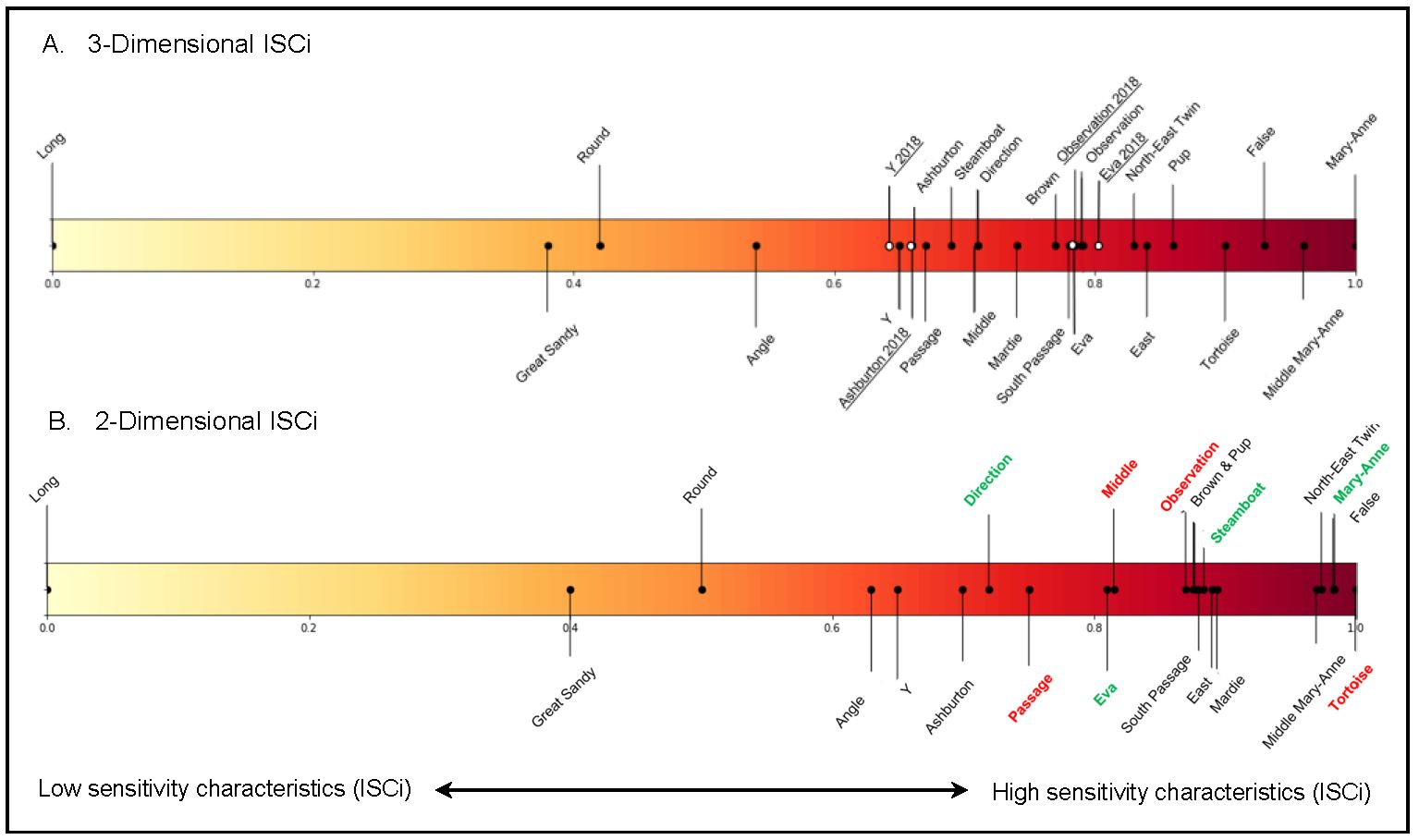
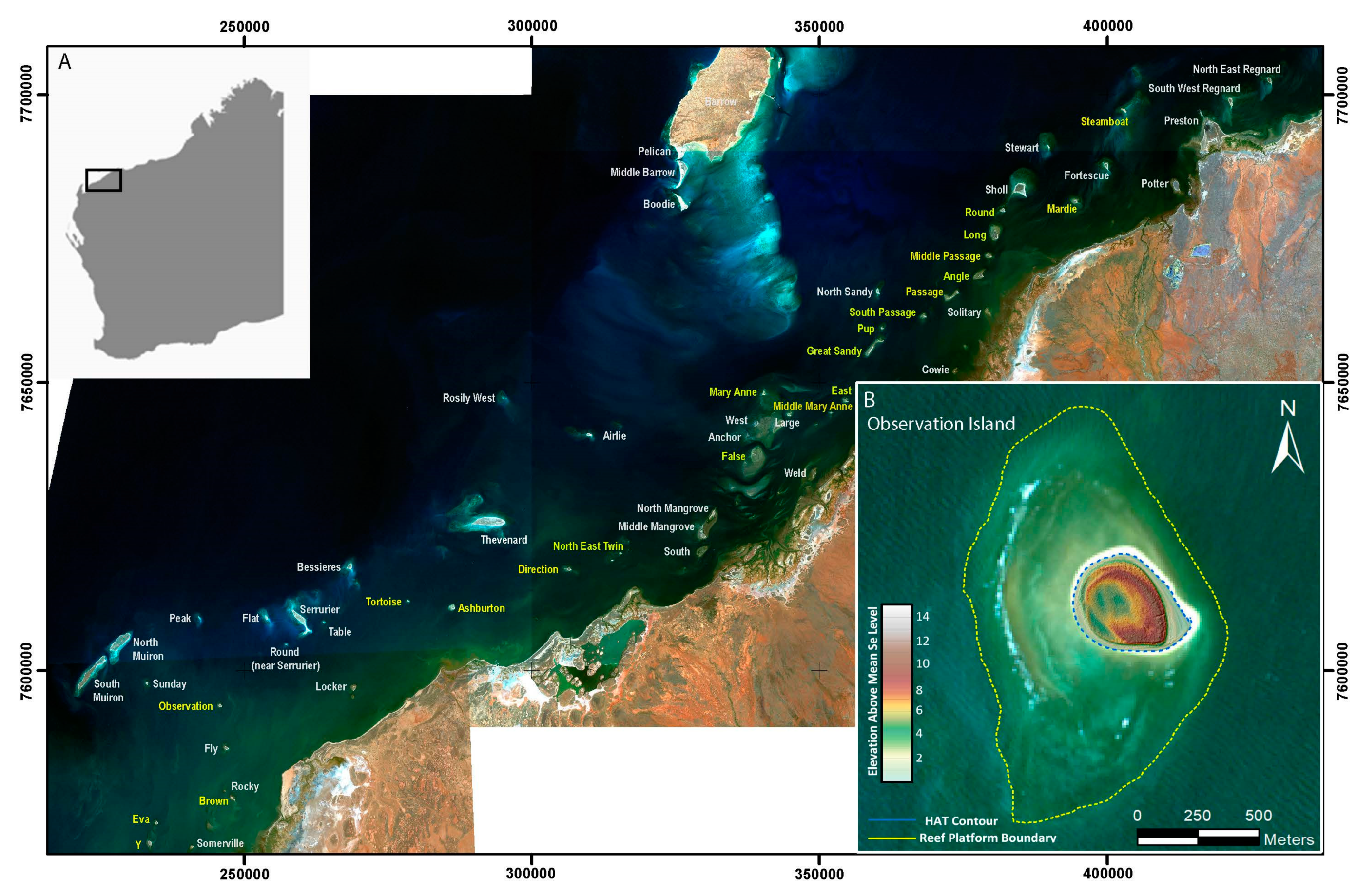
2.1. Regional Setting and Oceanography

The Pilbara islands, located in northwest Western Australia, are a chain of 64 uninhabited reef-fringed islands forming Australia’s largest sand-island archipelago. The island chain spans approximately 300 km along the Pilbara coastline, from Exmouth Gulf in the West to the Dampier Archipelago in the East (Figure 1). The region experiences S to SW winds for the majority of the year [15]. The regional wave climate is seasonally variable; winter is dominated by Southern Ocean swell that refracts along the inner shelf to approach the Pilbara coast from a NW direction, whilst the austral summer is dominated by locally generated wind-waves from the prevailing southerly winds [15]. The area also experiences strong episodic cyclone events (winds ≥ 90 km/h) occurring once every 2–3 years that produce damaging storm surge, swell, and winds. These extreme climatic conditions modify sediment supply and transport processes within the region, causing widespread coastal erosion, high turbidity, inundation, and landform destabilization [15,16,17].

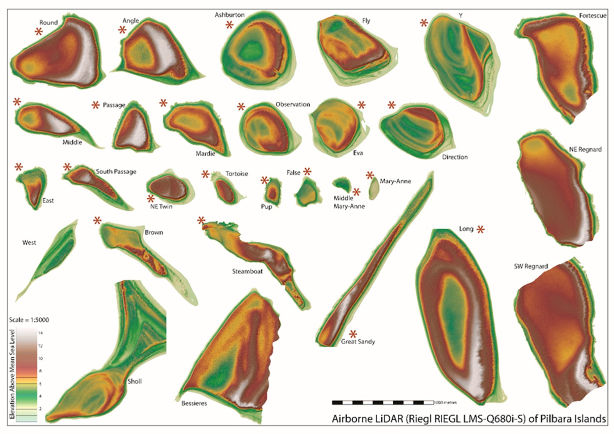
2.2. Acquisition of Island Morphometric Data

A total of 22 reef islands were mapped using a Riegl Q680i-S topographic LiDAR collected on 16 October 2016, and a follow-up survey for a sub-set of 4 (Eva, Y, Observation and Ashburton) were mapped on 11 October 2018 using both the Q680i-S and Riegl VQ820G Topo-Hydrographic (Figure 2). Both LiDAR systems were mounted in underwing pods on a Dimona (HK36TTC-ECO) motorglider-based research aircraft. In 2016, flying height was conducted at 1000 m amsl to cover all islands in one overpass, with the Q680 point densities between 3–5 points/m2. In 2018, LiDAR was flown at 600 m, with Q680 point densities between 10–12 points/m2, and combined Q680 and VQ820G densities of 30 points/m2. Vertical accuracy of the Q680 cloud was ± 10 cm. The LiDAR point cloud elevation was referenced to the Australian Height Datum (AHD) and was processed using the LAStools® (rapidlasso.com version 1.3) and BayesMap® Stripalign (version 1.6) to correct both relative and absolute geometric errors. The DEM was generated using the GlobalMapper® LiDAR module (version 19) “binning” process searching for the minimum values, with a search radius set to 10 (i.e., 10-times the mean data spacing). The DEM was exported as a 0.5 m DEM (2016 data) and 0.1 m DEM (2018 data) into ArcGIS® version 10.6 (ESRI® Brisbane, Australia, 2020) for analysis (Table S1). The 0.1 m 2018 DEM was converted to a 0.5 m resolution DEM (for improved processing time). Differential GPS (dGPS) ground control points (GCP’s) were collected on Eva, Y, Observation, and Ashburton islands and used to establish any elevation offset between the LiDAR derived DEM elevations and absolute GCP elevations. It was found that the 2016 LiDAR derived elevations were systematically 15 cm higher than the GCP and were corrected down by this value. The 2018 LiDAR derived DEM’s were within ± 10 cm of the GCP, therefore, no correction was applied. LiDAR data was captured during the spring high tides in 2016; therefore, it was not possible to use the mean sea level contour as a shoreline proxy. Instead, we used the highest astronomical tide (HAT) elevation, ranging from 1.3 m AHD (West) to 2.3 m AHD (East), reflecting the increasing tidal range across the Pilbara coastline. The HAT shorelines were used for the island 2D morphometrics and only data above the HAT datum was used for 3D morphometrics for both LiDAR datasets.

2.3. Island Geometry and Reef Platform

For the 22 islands, the reclassify tool in ArcMap® 10.6 (ESRI® Australia, 2020) was used to convert DEMs generated from the 2016 and 2018 LiDAR data to a polygon using the ‘raster to polygon’ feature to calculate island area (ha). To determine average island elevation (m), the DEMs for the islands were converted to a point feature using the conversion tool ‘raster to point’ feature. The ‘point data file’ derived from the point feature was then used to calculate island volume (m3) using the elevation at the grid cell multiplied by the pixel dimension (x, y) for each point data cell, and then summed (∑) to generate total island volume above HAT in cubic meters (m3). Elevation difference (i.e., surface difference) of Observation, Y, Eva, and Ashburton islands captured by the 2016 and 2018 LiDAR surveys was calculated using the ‘raster calculator’ function in ArcMap®. This was used to identify regions of elevation loss and/or gain by subtracting the islands 2016 DEM raster from the 2018 DEM raster. Due to the vertical accuracy of the surveys (±10 cm), only elevation differences of >20 cm were considered.
Reef platforms are important reef zones, acting as sediment factories (i.e., production and supply) for island construction and maintenance, and as sediment reservoirs [18,19]. As the 2016 survey only captured topographic LiDAR, and the 2018 topo-bathymetric LiDAR was only collected for four islands, we used an image-based approach to map the platform area for all 22 islands. We used Sentinel-2 imagery to identify the transition from reef flat to fore reef based on the distinctive change in color observed in the images (i.e., transition from light to dark when moving from shallow reef flat to deeper forereef). In ArcMap®, the ‘graphic polygon’ tool was used to trace the seaward edge of the reef platform (with the 2D polygon including the island landmass). The island areas (ha) were then subtracted from the area of the polygon to determine total reef platform area (ha). Although this is a subjective approach and dependent upon water clarity of the satellite images, repeated digitization by a single operator using Sentinel-2 images from a range of water quality scenarios showed a horizontal error of ±2 ha. To further test the accuracy and reproducibility of this approach, we verified the manual digitized platforms with the 2018 topo-bathymetric LiDAR. To delineate the edge of the reef platform from topo-bathymetric LiDAR, we calculated cross-shore profiles from the island shorelines to reef edge (depth of ±8 m) using the ‘interpolate line’ feature in ArcMap®. Here, we identified the platform boundary as the point where a change from horizontal to a negative change of slope occurs (i.e., transition from reef flat to fore reef slope). When manual and LiDAR-derived platform areas were compared, we found there to be a ±5 ha difference (<10% error). Given the error in our manual approach, this is not expected to effect the interpretation of results relying on this data. Linear regression analysis was performed in SPSS (SPSS Statistics version 22.0, IBM®, Armonk, New York, USA) to determine the relationship between (1) island area and island volume, and (2) reef platform area and island volume. Multiple linear regression was performed to determine the relationship between island area, island volume, and elevation.

2.4. Foredune Scarping and Island Orientation

Foredune scarping is a common erosional signature and occurs when a dune is eroded at its base causing the face to over steepen and collapse [20]. To estimate the length of island perimeter with foredune scarping we calculated the slope from the DEM and defined ‘scarping’ as slopes > 30°. This parameter was selected in accordance with the critical angle of repose for dry sand, which defined the angle where the upslope grains are no longer supported by the down slope grains and therefore sensitive to collapse [21]. Using the 3D analyst feature in ArcMap®, the slope tool was used to calculate the steepness for each cell of the raster surface (2016 0.5 m DEM; 2018 0.1 m DEM) for the 22 reef islands captured from the LiDAR survey. Slope is calculated as the maximum change in elevation over the distance between the cell and its eight neighbors, which identifies the steepest downhill descent from the cell (ESRI®, Brisbane, Australia, 2020). Therefore, areas were considered to have undergone scarping if there was continuous (>10 m alongshore) foredune with an angle > 30°. As a single island may exhibit more than one region with scarping > 30°, the geographic regions of these areas on each island were recorded (N, S, etc.). Areas with randomly distributed raster cells or interrupted bands of cells with angles > 30° were discounted, as they are not indicative of extended shoreface erosion.
Amount of orientation change at different timescales (seasonal, inter-annual) is an important characteristic of how dynamic an island is and its response to changing metocean and environmental conditions. Orientation of the major (or long) axis of the 22 islands captured from the 2016 and 2018 LiDAR was calculated in degrees (°) using the zonal geometry function (spatial analyst) tool in ArcMap® and was plotted on a polar plot for comparison against foredune perimeter slope angle (>30°).

2.5. Island Sensitivity Characteristics Index (ISCi)

The 22 islands were ranked according to an island sensitivity characteristics index based on their morphological attributes. Principle components analysis (PCA; SPSS Statistics version 22.0,IBM®, Armonk, New York, USA) was used to statistically ordinate the 2016 LiDAR data (for the 22 islands) and 2018 LiDAR (for the 4 additional islands) on (1) island area, (2) reef platform area, (3) island volume, (4) average island elevation, and (5) foredune scarping for all islands. These characteristics were chosen based on their importance as potential indicators of both contemporary and long-term island erosion and accretion. PCA is a statistical method that implements orthogonal transformation to convert a set of observations of possibly correlated variables into a set of linearly uncorrelated variables called principal components (PCs), with the PC1 explaining the maximum amount of variation in the data. An island sensitivity characteristics index (ISCi) was generated using the factor scores derived from PC1, normalized to a range between 0 and 1, representing the least (0) and most (1) sensitive island in the analysis. An index score close to 0 signified islands with low sensitivity characteristics (larger island, larger platform area, larger volume, higher elevation, and less extensive scarping) and a score close to 1 signified islands with high sensitivity characteristics (smaller island, smaller reef platform area, lower volume, lower elevation, and more extensive scarping). To determine change over time (2016 to 2018) for Eva, Y, Ashburton, and Observation, the 2018 morphometric characteristics (as mentioned above) were included in the PCA and the ordination re-calculated to determine the new index value.

2.6. Validation of 3D Versus 2D Orphometrics in ISCi Interpretation

To statistically validate the accuracy of using 3D over 2D morphometric variables in interpreting island sensitivity using the newly developed ISCi, a separate PCA was conducted using only 2D morphometrics (island area and reef platform area) to compare against the full 3D ISCi index. Our aim was to determine whether 3D morphometric characteristics were more strongly correlated (i.e., strongly influence) with the ISCi values generated for the 22 islands compared to 2D characteristics only. Using the PC1 components matrix generated from the 2D PCA, the strength of the correlation for each morphometric characteristic was denoted by a value < 1 (where values approaching 1 explain more variability). The factor scores derived from the PC1 of the 2D PCA were then used to generate an indexed ranking of islands (methodology as per Section 2.5) and compared to the positioning of islands (based on their sensitivity characteristics) along the index against the full 3D ISCi.

3. Results

3.1. Variability of Island Morphometrics

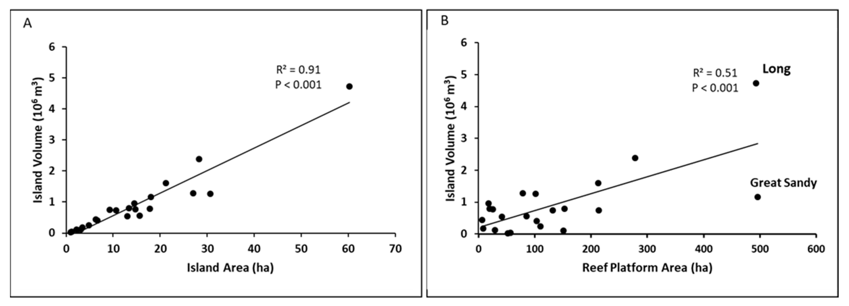
3.1.1. Relationship between Island Area, Volume, and Elevation

The 22 islands collectively exhibited an island area ranging from 0.9–60.2 ha, a reef platform area ranging from 6.1–495.3 ha, and an island volume ranging from 19,522–4,723,208 m3. Island area (p < 0.001, R2 = 0.91) was a strong predictor, and reef platform area (p < 0.001, R2 = 0.51) a moderate predictor of island volume (Table 1; Figure 3). Great Sandy and Long islands were found to deviate from the platform area/volume relationship. Great Sandy exhibited a small island area (18.0 ha) and volume (1,157,551 m3), yet was situated on a large reef platform of 495.3 ha. Long island however, is situated on a similarly large reef platform (493.0 ha), with a large island area (60.2 ha) and greater than predicted island volume (4,723,208 m3). Results from a multiple linear regression analysis indicate island area and island volume to be moderate predictors of island elevation (p < 0.05, R2 = 0.48).

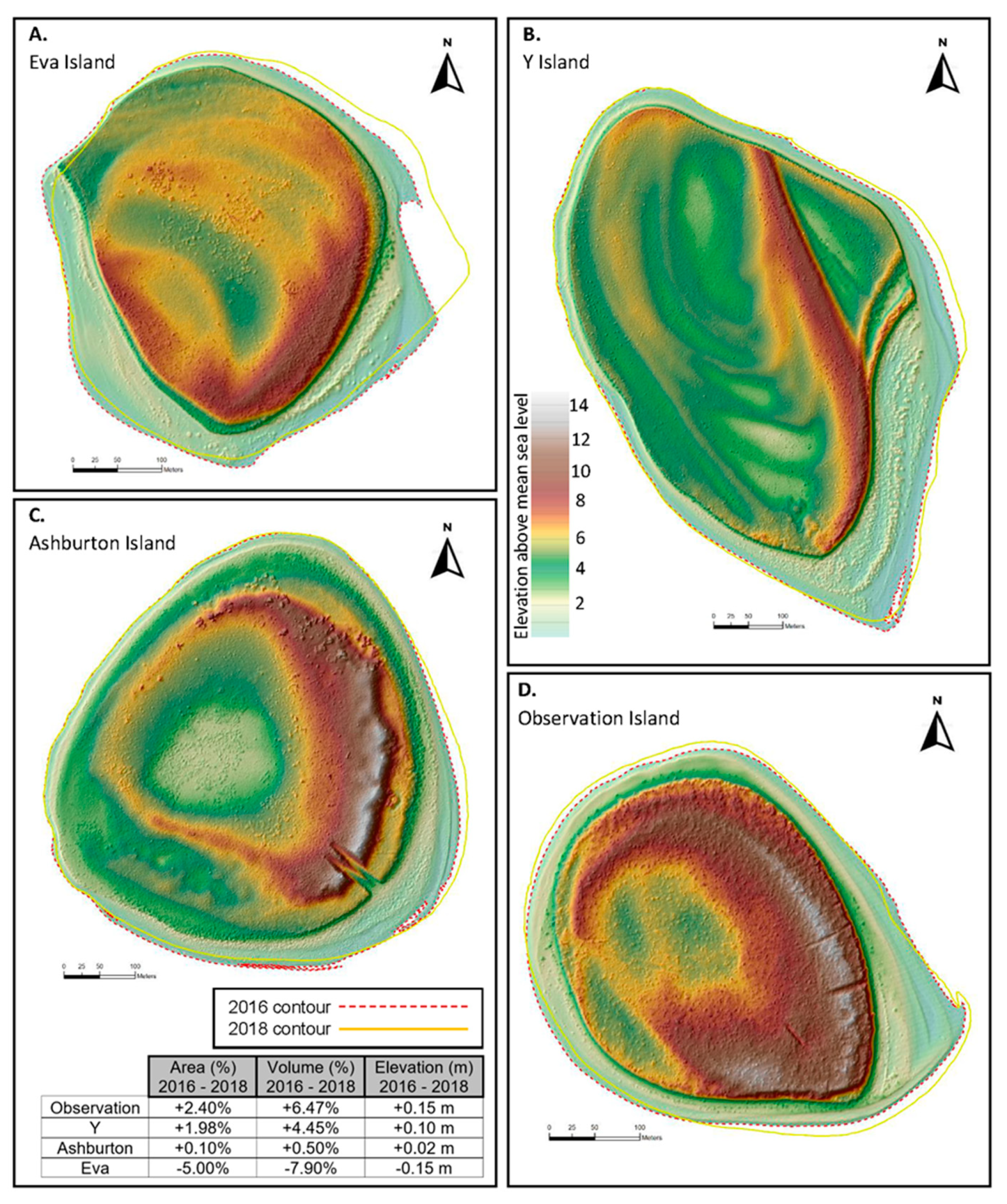
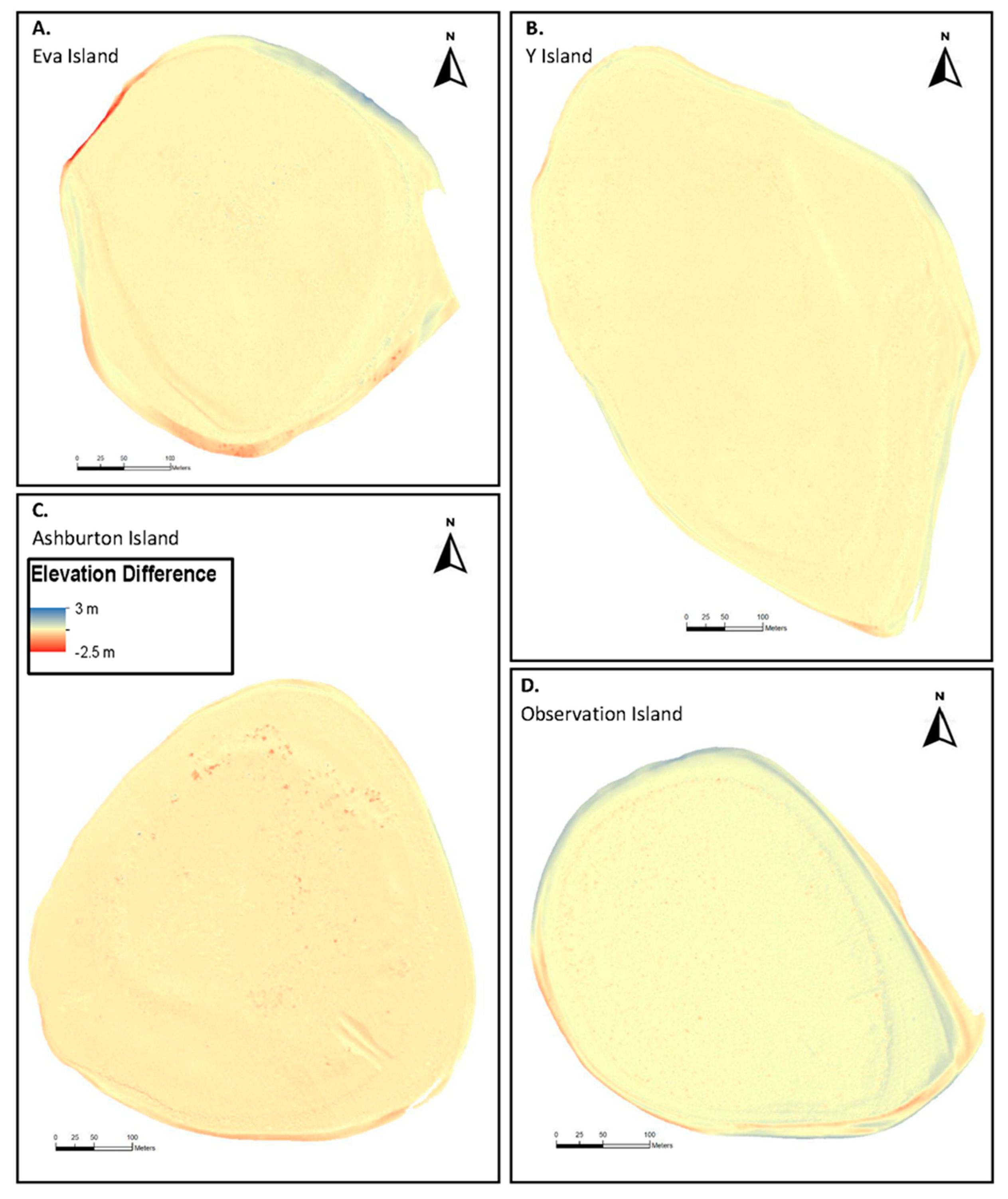
3.1.2. Change in Island Area, Volume, and Elevation over a 2-Year Period (2016–2018)

LiDAR imagery captured during October of 2016 and 2018 was used to generate data on change in island area (ha), island volume (m3), and average island elevation (m) for Eva, Y, Observation, and Ashburton islands over a 2-year time period (Figure 4). Analysis of island change showed that 3 islands experienced a minor increase in area (0.5 to 2.5%), with Observation island exhibiting the greatest overall gain, followed by Y and Ashburton. Eva island however, experienced a reduction in island area (5%). Eva exhibited landform loss on its north-western and southern shorelines, and expansion on its north-eastern and eastern shorelines, with a total land loss of 0.78 ha. Ashburton exhibited landform loss on its southern shorelines and expansion on the eastern side, with a total land gain of 0.04 ha (0.10%). Y island showed expansion on its eastern and south-eastern shorelines and planform loss on its southern with an area increase of 0.61 ha (1.98%). Lastly, Observation, which is the smallest of the 4 islands, was shown to have contracted on its south-western and north-eastern shorelines and expansion on its southern, south-eastern, and north-western shorelines with a total area gain of 0.36 ha (2.40%).
Changes in island area among islands correlated with changes in island volume and elevation. Eva decreased in volume by 8% (−42,484 m3), Ashburton saw only a 0.5% increase in volume (+6484 m3), whereas Y and Observation increased in volume by 4.4% (+56,460 m3) and 6.4% (+50,078 m3), respectively (Figure 4). Islands that gained volume (Observation, Y, and Ashburton) also increased in average elevation. Observation showed the highest increase in average elevation by 0.15 m, followed by Y at 0.10 m and Ashburton with an increase by 0.02 m. In contrast, Eva exhibited a decrease in average elevation by 0.15 m above the HAT (Figure 4). Although these average elevation changes are minor (and within the DEM vertical error range of ± 0.10 m), there are however large sections of these islands (upper beachface/foredune) that show large and measureable change (vertical changes of ± 2 m), whereas higher elevation portions of the islands (‘island core”) remained stable (Figure 5).

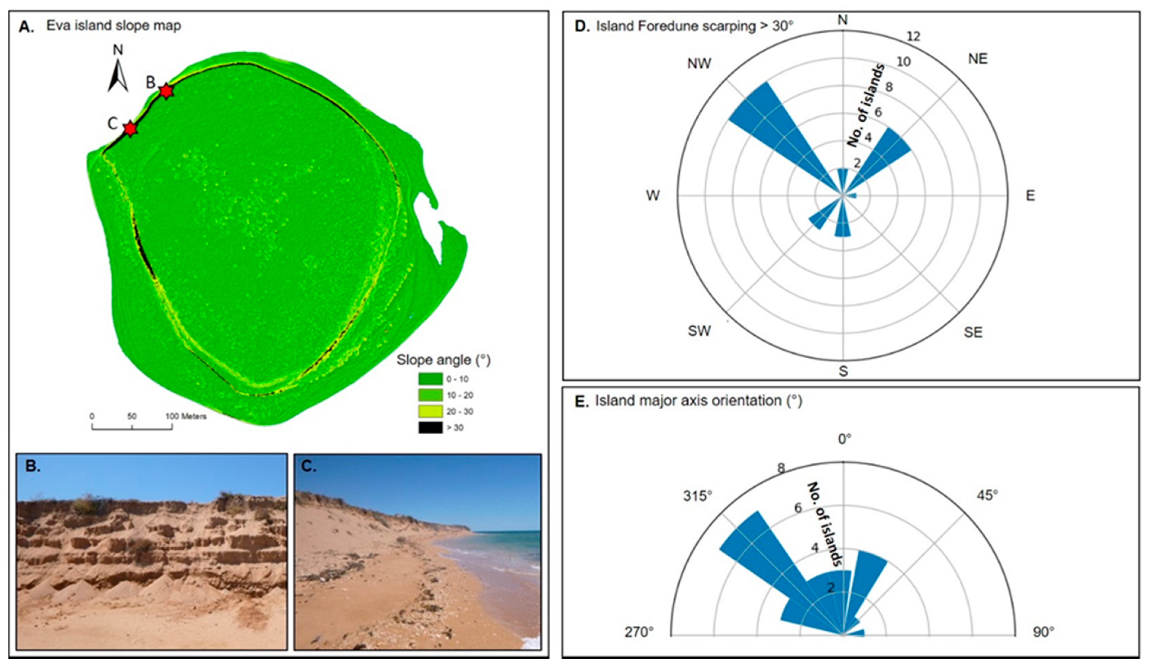
3.1.3. Foredune Scarping and Island Orientation

Most of the islands (16 of 22) exhibited foredune scarping along their northern (NW-N-NE) shorelines (Figure 6). Six islands (Great Sandy, Mardie, Mary Anne, Ashburton, and Middle Mary Anne) showed no significant scarping (>30°) along their shoreline perimeter. In addition, 20 of 22 islands had their major axis orientated to the N and NW (3°–357°; Figure 6E). The 2 remaining islands (Great Sandy and Round) were shown to exhibit a NE major axis (34°& 74°; Figure 6E).

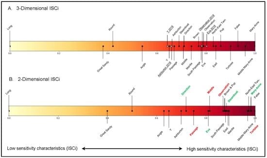
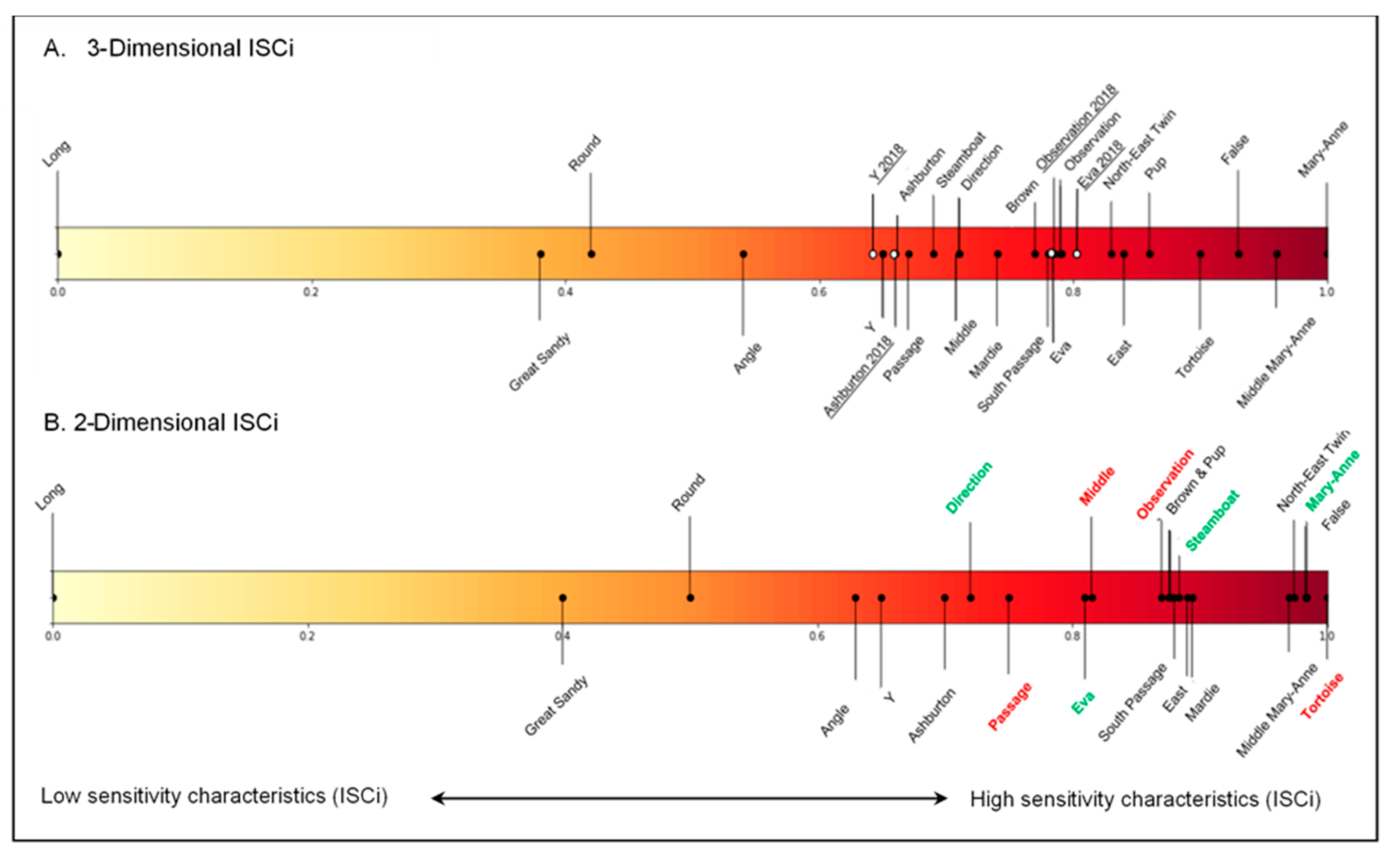
3.2. Island Sensitivity Characteristics Index (ISCi)

The first principle component (PC1) explained 73% of the total variance among islands (λ1 = 3.63), and is strongly influenced by island volume (0.94), island area (0.90), extent of foredune scarping (0.87), reef platform area (0.85) and average island elevation (0.66) (values in parentheses approaching 1 have a greater influence). Of the 22 islands, Long, Great Sandy, Round, and Angle exhibited a lower island sensitivity index value (ISCi < 0.6), characterized by large island volume and area, limited foredune scarping, and high average elevation (e.g., >7 m AHD) (Figure 7). Mary Anne, Middle Mary Anne, False, Tortoise, Pup, and East and NE Twin islands exhibited higher index values (ISCi between 0.8–1), characterized by small island volume and island area, extensive scarping, and relatively low average elevations (e.g., <7 m AHD). The remaining 12 islands had an ISCi value ranging between 0.6 > ISCi < 0.8. Of the 4 islands compared across 2016 and 2018, Ashburton island showed no change in sensitivity characteristics over the 2 years (ISCi 2016/2018 = 0.66), whereas Eva showed a minimal increase in sensitivity characteristics (’16 = 0.78, ’18 = 0.8) due to smaller island area, smaller volume, lower elevation, and more extensive scarping. Y and Observation declined by 1% (0.01) to 0.65 and 0.78, respectively. As such, all islands can be considered to be in a relatively stable condition during this 2-year timeframe.

3.3. Accuracy of 3D Morphometrics in ISCi Interpretation

Results show the full 3D ISCi (island area, platform area and volume, perimeter scarping, and average elevation) to better represent differences between islands compared to the 2D ISCi (island area, platform area) (Figure 7). In the 2D PCA, island area and platform area were strongly correlated to the ISCi values (0.9). However, the addition of 3D morphological characteristics (i.e., volume, perimeter scarping and elevation), showed volume to be the greatest driving influence on the ISCi followed by island area, perimeter scarping, platform area, and lastly, average elevation (see Section 3.2 value in parentheses). Importantly, addition of the 3D characteristics changed the order of islands along the ISCi compared to the 2D ISCi. This suggests that the inclusion and interaction of these 3D variables is important for accurately determining the relative island sensitivities to change. Selected examples include; (1) Tortoise, which recorded the highest sensitivity value (ISCi = 1) in the 2D ISCi, whereas Mary Anne exhibited the highest sensitivity value (ISCi = 1) in the 3D ISCi, (2) Observation, which recorded a higher sensitivity value than Steamboat in the 2D ISCi, whereas Steamboat exhibited a higher sensitivity value than Observation in the 3D ISCi, (3) Middle, which recorded a higher sensitivity value than Eva in the 2D ISCi, and the lower sensitivity in the 3D ISCi and lastly, (4) Direction, which recorded a lower sensitivity value than Passage in the 2D ISCi, and higher sensitivity in the 3D ISCi; Figure 7

4. Discussion

4.1. Morphometric Characterization

We observed a strong positive relationship between reef platform area and island volume. Reef platforms are key reef environments for sediment production (i.e., breakdown of carbonate producers/reefal framework) and temporary sediment storage (i.e., of relict sediments) [22]; therefore, the relationship between platform area and volume suggests that larger platforms generate a larger and more readily available sediment reservoir for island development and accretion [4,23]. Further, larger coral reef platforms have the potential to reduce incident wave energy reaching island shorelines by increasing wave attenuation via breaking and frictional dissipation [24]. Therefore, larger platforms protect island shorelines against incident swell that might otherwise result in island erosion during high and/or low energy events [25].
The significant relationship between reef platform area and island volume may help to broadly identify islands whose reef platforms are capable of maintaining island sediment budgets or islands that may be experiencing a net sediment supply deficit. For example, where island volume is lower than predicted for a given reef platform area, (e.g., Great Sandy), this may indicate that this island is either susceptible to active erosion or may be in an early developmental/evolutionary stage. In contrast, where island volume is higher than predicted for a given reef platform area (e.g., Long), this may indicate a reef platform environment with a particularly high carbonate sediment production rate. Thus, observed departures from the linear relationships (Figure 3) could suggest changes in carbonate sediment production rates and/or sediment supply and availability as one potential driver of island maintenance related to ecological and/or metocean processes.
Digital elevation models show distinctive evidence of foredune scarping, an erosional signature that align to the NW, N, and NE of the islands (Figure 6A–D). This result is also consistent with the island major axis orientation (Figure 6E). Both the scarping regions and island major axis orientations align with the dominant swell direction of the region after refracting around the North-West Cape [15,26]. This relationship suggests that the incident swell is eroding northern shorelines and transporting sediment alongshore to deposit at nodal points on the southern shorelines of the islands [27]. No major high energy events (i.e., cyclones) were reported across the Pilbara during the 2016–2018 timeframe. Therefore, measured changes are likely (or could only) be the result of prevailing (‘fair-weather’) incident conditions. Comparison of the high-resolution airborne LiDAR surveys captured in October of 2016 and 2018 for the 4 islands (Observation, Y, Eva, and Ashburton) suggest that the islands are stable, yet exhibit a variety of island shoreline adjustments. Areas of volume and elevation change were found to correspond to foredune accretion (i.e., volume and elevation gain) and regions of foredune erosion/scarping (i.e., volume and elevation loss) (Figure 4 and Figure 5). Further, shoreline accretion generally occurred on the eastern shorelines of the islands. This shoreline extension is shown to align with the seasonal variability in wave and wind climate, which predominantly occur from the west (i.e., NW or SW). This is influenced by Southern Ocean swell waves refracting around the North West Cape and entering the Exmouth Gulf from a NW direction during the austral winter [15] and local generated wind-waves from the prevailing southerlies during the austral summer.
Here, we highlight the capability of LiDAR technology to directly identify those islands experiencing active or recent erosion and/or accretion from a single time point survey (i.e., one data collection). Results show that regions of foredune scarping (e.g., as identified on NW island shorelines) can be rapidly identified and quantified from a single LiDAR dataset, providing an accurate and detailed assessment of those region/s of the island landmass experiencing erosion and instability that would otherwise require several independent time points to measure using traditional 2D aerial and satellite imagery. This result presents an important capability of LiDAR and other 3D datasets, providing a rapid assessment of: (1) sensitive geomorphic regions and their alignment/orientation and, (2) its influence on island geomorphic state at the time of survey, which could help to better predict the effect from potential metocean and environmental drivers (e.g., local wind/wave climate). Importantly, these finding would not be possible from a single survey collection of historical aerial and satellite imagery as it required the use of 3D measurements to identify these geomorphic features.

4.2. Island Sensitivity Characteristics Index (ISCi) and Implications for Island Stability

Island morphometric data was used to generate an island sensitivity characteristics index (ISCi) (Figure 7). The objective of this index is to provide broad evaluation of island morphological state at the time of data collection and can be implemented as a relative and preliminary diagnostic indicator of comparable island instability. Islands with a high sensitivity characteristics index (where ISCi → 1; Figure 7) were characterized by small areas and volumes, low elevations, smaller reef platform areas, and extensive scarping. It is the combined influence of these morphological characteristics that can point to island instability and a greater potential risk of these islands to experience inundation, shoreline erosion, and landform destabilization [28,29,30]. The index decreases (where ISCi → 0; Figure 7) as islands exhibit less sensitive characteristics due to increasing areas and volumes, high elevations, and less extensive scarping. The combination of these characteristics indicates that these islands are relatively more resilient and stable. Further, the index shows no regional pattern across the archipelago, suggesting that the variability in island sensitivity is linked to local island characteristics (e.g., island developmental history, reef productivity/health, and contemporary sediment supply) and environmental drivers (e.g., local wind/wave conditions). This suggests that management of these islands that seek to promote and maintain island resilience to future climate changes needs to include site specific solutions, yet has the potential to be effective at prioritizing islands more in need of management.
Between the years 2016 and 2018, the sensitivity index for all the 4 islands (Observation, Y, Eva, and Ashburton) remained relatively unchanged, suggesting all islands to be stable or in a state of geomorphic equilibrium. Observation and Y recorded an increase in island volume and average elevation, with a small increase in island area, potentially suggesting vertical island accretion. In comparison, Ashburton remained unchanged (i.e., no change in sensitivity index) across the two years, consistent with little to no increase in island volume, elevation and area, suggesting the island to be more geomorphically stable (i.e., exhibiting neither a net loss nor gain in sediment). Lastly, Eva recorded an increase to its ISCi value (i.e., shift towards higher sensitivity characteristics). Unlike its counterparts, Eva recorded a decrease in island area, volume, and elevation, potentially suggesting net island erosion (i.e., exhibiting a net loss of sediment). Shoreline retreat from 2016 to 2018 on the NW and southern shorelines of Eva support this trend, with a decrease in island area and elevation. Here, sediment was deposited at lower elevations (i.e., eastern shorelines), where it is more readily available for transport out of the system and the island’s sediment budget.

Accuracy of 3D Versus 2D Morphometrics in ISCi Interpretation

The 3D morphometric characteristics used in the 3D PCA were strongly correlated with the ISCi, with island volume being the strongest driver of the index. As such, the 2D ISCi ranked islands in a different order than the 3D ISCi. For example, Tortoise is ranked the most sensitive island on the 2D ISCi, whereas Mary Anne is ranked most sensitive on the 3D ISCi. Mary Anne exhibits a significantly smaller island volume (~150,000 m3 difference), area, and elevation (3.3 m lower) than Tortoise, exhibiting higher sensitivity characteristics. Yet, this sensitivity is not captured using the 2D ISCi. Further, according to the 2D ISCi, Steamboat exhibits a higher sensitivity characteristics index value than Observation, influenced by its smaller island and reef platform area. However, the ranking is inverted on the 3D ISCi, with Steamboat exhibiting higher total volume (~200,000 m3 difference), elevation (0.7 m higher), and a lower scarped perimeter than Observation. These results suggest that the use of only 2D morphometrics (i.e., island area and platform area) in assessing island landform sensitivities may lead to inaccurate interpretations on the ranking of islands according to sensitivity characteristics. In view of this, our findings highlight what can be achieved from a single pass 3-dimensional LiDAR survey, and how this data may expand on and complement existing 2D LiDAR datasets.
This is the first study to propose an index ranking of reef islands based on 3D sensitivity characteristics. Yet, further development and validation of this index to include in-situ non-morphometric parameters, such as island age/developmental history, hydrodynamic energy and inundation potential, and contemporary sediment production rates will provide a more holistic assessment of sensitivity. This understanding will be crucial for forecasting short and long-term trajectories of reef-island stability and a better quantification of island sensitivity thresholds to changing climate. The benefit of this approach is a rapid, broad spatial scale assessment of island sensitivity, and with further development, may be applied alongside ecological and ethnographic datasets to prioritize management outcomes of both island landforms, human economics, and the ecological value of their terrestrial and benthic coral reef ecosystems.

5. Conclusions

This was the first systematic study to assess the geomorphic sensitivity of reef islands to changing metocean conditions using regional-scale LiDAR. The results suggest a significant influence of reef platform area on total island volume, indicating its critical role as a carbonate sediment factory, and/or as an active barrier against wave-driven shoreline erosion. LiDAR has also enabled the rapid assessment of morphodynamically active regions (scarped areas) from a single data collection, which would typically require a time series of imagery for a more classical 2D analysis approach. In general, our results highlight the advantages of a 3D snapshot of islands that enables identification of area, volume, elevations, and morphodynamically active regions.
A new metric termed the island sensitivity characteristics index (ISCi) allows the assessment of island’s contemporary morphological state based on a suite of morphometric characteristics. High ISCi values suggest islands have greater sensitivity characteristics (i.e., small island volume and area, and small reef platform area, low elevation, and greater perimeter scarping > 30°), whereas low ISCi suggests islands with lower degree of sensitivity characteristics. Consequentially, the ISCi has the potential for assessing relative changes in morphological stability of islands in response to climate change as well as an important tool in informing adaptive management strategies. Ongoing use of LiDAR and other 3D technology (e.g., UAVs) for monitoring reef islands will help to more accurately quantify their resilience to future climate change given the synergistic impacts of global environmental change and the threat to the ecology and human economics of reef islands worldwide.

Supplementary Materials

The following are available online at https://www.mdpi.com/2072-4292/12/18/3033/s1, Figure S1: Methodology flow chart (including processing and analysis of DEM and Sentinel-2 imagery), Table S1: Tidal data corresponding to 22 islands survey during October 2016. Contour elevation of each island (m, AHD) compared against Highest Astronomical Tide (HAT) across the island archipelago, Table S2: Table of morphometric data for the 22 Pilbara reef islands. Data includes island area (ha), Reef platform area (ha), island volume (m3), Average and maximum elevation (m), perimeter scarping and island major axis orientation, Table S3: Table of morphometric data for the 22 Pilbara reef islands gathered from 2016 LiDAR used in the Principle components analyses. Factor scores derived from the PCA were normalised to generate an indexed value range between 1 and 0 (1 being high sensitivity characteristics and 0 low sensitivity characteristics), Table S4: Statistical results of PCA explaining total variance explained and components matrix (strength of individual parameters), Table S5: Table of morphometric data for the 22 Pilbara reef islands gathered from 2016 LiDAR used in the Principle components analyses. 2018 LiDAR data for 4 islands (Eva, Obs, Ashburton and Y) included to calculate change in ISCi between 2016 and 2018. Factor scores derived from the PCA were normalised to generate an indexed value range between 1 and 0 (1 being high sensitivity characteristics and 0 low sensitivity characteristics).

Author Contributions

Conceptualization, J.L.B., M.O., M.V.W.C., and N.B.; methodology, J.L.B., M.O., M.V.W.C., N.B., and J.H.; software, M.O., and M.V.W.C.; formal analysis, J.L.B.; investigation, J.L.B.; resources, J.H., M.O., and N.B.; data curation, J.L.B., M.O, and J.H.; writing—original draft preparation, J.L.B., M.V.W.C., M.O., and N.B.; writing—review and editing, J.L.B., M.V.W.C., M.O., and N.B.; visualization, J.L.B.; supervision, M.V.W.C., M.O., and N.B.; project administration, M.O.; funding acquisition, N.B. and M.O. All authors have read and agreed to the published version of the manuscript.

Funding

This research study was supported by an Australian Research Council (ARC) Discovery Project DP160102561; and a DECRA Fellowship DE180100391 awarded to Nicola Browne of Curtin University, Perth, as part of the island resilience project (2018–2020).

Acknowledgments

The authors would like to thank Shakti Chakravarty for aircraft logistics and operating instrumentation on-board research motorglider. JB would like to cordially thank the advice of Ethan Chaffey, Adi Zweifler, and Mario Conde-Frias on manuscript drafts, Shannon Dee for boating operations, and Chris Whitwell and Renan Di Silva on valuable advice on Python and MatLab coding for figure conception and creation. We also thank the regional Exmouth office of the West Australian government Department of Biodiversity, Conservation and Attractions (DBCA) for their ongoing support and the Minderoo Foundation for providing funding and logistical sponsorship through the Minderoo Exmouth Research Lab (MERL) facility, Exmouth. Lastly, thank you to Erica Ashe, Rutgers University, for statistical advice on the analyses of data.

Conflicts of Interest

The authors declare no conflict of interest.

References

  1. Duvat, V.K.; Pillet, V. Shoreline changes in reef islands of the Central Pacific: Takapoto Atoll, Northern Tuamotu, French Polynesia. Geomorphology 2017, 282, 96–118. [Google Scholar] [CrossRef]
  2. Kench, P.S.; Thompson, D.; Ford, M.R.; Ogawa, H.; McLean, R.F. Coral islands defy sea-level rise over the past century: Records from a central Pacific atoll. Geology 2015, 43, 515–518. [Google Scholar] [CrossRef]
  3. McLean, R.; Kench, P. Destruction or persistence of coral atoll islands in the face of 20th and 21st century sea-level rise? Wiley Interdiscip. Rev. Clim. Chang. 2015, 6, 445–463. [Google Scholar] [CrossRef]
  4. Perry, C.T.; Kench, P.S.; Smithers, S.G.; Riegl, B.; Yamano, H.; O’Leary, M.J. Implications of reef ecosystem change for the stability and maintenance of coral reef islands. Glob. Chang. Biol. 2011, 17, 3679–3696. [Google Scholar] [CrossRef]
  5. East, H.; Perry, C.T.; Kench, P.S.; Liang, Y.; Gulliver, P. Coral reef island initiation and development under higher than present sea levels. Geophys. Res. Lett. 2018, 45, 11–265. [Google Scholar] [CrossRef] [Green Version]
  6. Bryson, M.; Duce, S.; Harris, D.; Webster, J.M.; Thompson, A.; Vila-Concejo, A.; Williams, S.B. Geomorphic changes of a coral shingle cay measured using kite aerial photography. Geomorphology 2016, 270, 1–8. [Google Scholar] [CrossRef]
  7. Lowe, M.K.; Adnan, F.A.F.; Hamylton, S.M.; Carvalho, R.C.; Woodroffe, C.D. Assessing reef-island shoreline change using UAV-derived orthomosaics and digital surface models. Drones 2019, 3, 44. [Google Scholar] [CrossRef] [Green Version]
  8. Turner, I.L.; Harley, M.D.; Drummond, C.D. UAVs for coastal surveying. Coast. Eng. 2016, 114, 19–24. [Google Scholar] [CrossRef]
  9. Hamylton, S.M. Mapping coral reef environments: A review of historical methods, recent advances and future opportunities. Prog. Phys. Geogr. 2017, 41, 803–833. [Google Scholar] [CrossRef]
  10. Sallenger, A., Jr.; Krabill, W.B.; Swift, R.N.; Brock, J.; List, J.; Hansen, M.; Holman, R.A.; Manizade, S.; Sontag, J.; Meredith, A.; et al. Evaluation of airborne topographic lidar for quantifying beach changes. J. Coast. Res. 2003, 19, 125–133. [Google Scholar]
  11. Carrivick, J.L.; Smith, M.W.; Quincey, D.J. Structure from Motion in the Geosciences; John Wiley & Sons: Hoboken, NJ, USA, 2016. [Google Scholar]
  12. Buckley, S.; Vallet, J.; Braathen, A.; Wheeler, W. Oblique helicopter-based laser scanning for digital terrain modelling and visualisation of geological outcrops. Int. Arch. Photogramm. Remote Sens. Spat. Inf. Sci. 2008, 37, 493–498. [Google Scholar]
  13. Terefenko, P.; Zelaya Wziątek, D.; Dalyot, S.; Boski, T.; Pinheiro Lima-Filho, F. A high-precision LiDAR-based method for surveying and classifying coastal notches. ISPRS Int. J. Geo-Inf. 2018, 7, 295. [Google Scholar] [CrossRef] [Green Version]
  14. Xhardé, R.; Long, B.; Forbes, D. Accuracy and limitations of airborne LiDAR surveys in coastal environments. In Proceedings of the IEEE International Symposium on Geoscience and Remote Sensing, Denver, CO, USA, 31 July–4 August 2006. [Google Scholar]
  15. Dufois, F.; Lowe, R.J.; Branson, P.; Fearns, P. Tropical cyclone-driven sediment dynamics over the Australian North West Shelf. J. Geophys. Res. Ocean. 2017, 122, 10225–10244. [Google Scholar] [CrossRef] [Green Version]
  16. Steedman, R.; Russell, K. Storm Wind, Wave and Surge Analysis, Exmouth Gulf, Western Australia; Steedman Ltd.: Perth, Australia, 1986. [Google Scholar]
  17. Twiggs, E.J.; Collins, L.B. Development and demise of a fringing coral reef during Holocene environmental change, eastern Ningaloo Reef, Western Australia. Mar. Geol. 2010, 275, 20–36. [Google Scholar] [CrossRef]
  18. Perry, C.T.; Morgan, K.M.; Yarlett, R.T. Reef habitat type and spatial extent as interacting controls on platform-scale carbonate budgets. Front. Mar. Sci. 2017, 4, 185. [Google Scholar] [CrossRef] [Green Version]
  19. Dee, S.; Cuttler, M.; O’Leary, M.; Hacker, J.; Browne, N. The complexity of calculating an accurate carbonate budget. Coral Reefs 2020, 39, 1–10. [Google Scholar] [CrossRef]
  20. Conaway, C.A.; Wells, J.T. Aeolian dynamics along scraped shorelines, Bogue Banks, North Carolina. J. Coast. Res. 2005, 21, 242–254. [Google Scholar] [CrossRef]
  21. Titus-Glover, L.; Fernando, E.G. Evaluation of Pavement Base and Subgrade Material Properties and Test Procedures; Texas Transportation Institute: College Station, TX, USA, 1995; pp. 1–126.
  22. Yamano, H.; Kayanne, H.; Chikamori, M. An overview of the nature and dynamics of reef islands. Glob. Environ. Res. Engl. Ed. 2005, 9, 9. [Google Scholar]
  23. Perry, C.T.; Kench, P.S.; O’Leary, M.J.; Morgan, K.M.; Januchowski-Hartley, F. Linking reef ecology to island building: Parrotfish identified as major producers of island-building sediment in the Maldives. Geology 2015, 43, 503–506. [Google Scholar] [CrossRef]
  24. Lowe, R.J.; Falter, J.L.; Bandet, M.D.; Pawlak, G.; Atkinson, M.J.; Monismith, S.G.; Koseff, J.R. Spectral wave dissipation over a barrier reef. J. Geophys. Res. Ocean. 2005, 110, 1–16. [Google Scholar] [CrossRef]
  25. Cuttler, M.V.W.; Hansen, J.E.; Lowe, R.J.; Drost, E.J.F. Response of a fringing reef coastline to the direct impact of a tropical cyclone. Limnol. Oceanogr. Lett. 2018, 3, 31–38. [Google Scholar] [CrossRef]
  26. May, S.M.; Brill, D.; Leopold, M.; Callow, J.N.; Engel, M.; Scheffers, A.; Opitz, S.; Norpoth, M.; Bruckner, H. Chronostratigraphy and geomorphology of washover fans in the Exmouth gulf (NW Australia)—A record of tropical cyclone activity during the late Holocene. Quat. Sci. Rev. 2017, 169, 65–84. [Google Scholar] [CrossRef]
  27. Gourlay, M.R. Coral cays: Products of wave action and geological processes in a biogenic environment. In Proceedings of the 6th International Coral Reef Symposium, Townsville, Australia, 8–12 August 1988. [Google Scholar]
  28. Beetham, E.; Kench, P. Predicting wave overtopping thresholds on coral reef-island shorelines with future sea-level rise. Nat. Commun. 2018, 9, 1–8. [Google Scholar] [CrossRef]
  29. Kumar, L.; Eliot, I.; Nunn, P.D.; Stul, T.; McLean, R. An indicative index of physical susceptibility of small islands to coastal erosion induced by climate change: An application to the Pacific islands. Geomat. Nat. Hazards Risk 2018, 9, 691–702. [Google Scholar] [CrossRef]
  30. Shope, J.B.; Storlazzi, C.D. Assessing morphologic controls on atoll island alongshore sediment transport gradients due to future sea-level rise. Front. Mar. Sci. 2019, 6, 245. [Google Scholar] [CrossRef] [Green Version]
Figure 1. (A) Map of Pilbara islands; those 22 islands examined in the study are labelled yellow. (B) Example digital elevation model (DEM) of Observation Island showing highest astronomical tide (HAT) contour (blue dashed line) and reef platform area (yellow dashed line). White area around contour line is subaerial sand captured in the satellite image, but not captured by LiDAR due to tidal level at time of flight. Coordinates reported in UTM Zone 50, axis in meters (m).
Remotesensing 12 03033 g001
Figure 2. Schematic representing the Pilbara reef islands surveyed using terrestrial airborne LiDAR during October of 2016. The N = 22 islands marked by a red asterisk (*) had complete sub-aerial LiDAR data and were used in the analyses. The remaining islands had incomplete LiDAR data, and therefore were excluded from the analyses.
Remotesensing 12 03033 g002
Figure 3. Linear regression of (A) island area versus island volume and (B) reef platform area vs. island volume for the 22 islands surveyed in October 2016.
Remotesensing 12 03033 g003
Figure 4. Changes in island area, island volume, and average island elevation for (A) Eva, (B) Y, (C) Ashburton, and (D) Observation islands (between 2016 to 2018) using the 0.5 m digital elevation models (DEMs). The 2016 island area is defined as the HAT contour marked by the red dashed line and the 2018 island area marked as the yellow solid line. High-resolution LiDAR was captured during October of 2016 and 2018.
Remotesensing 12 03033 g004
Figure 5. Surface difference between 2016 and 2018 illustrating elevation (m) gain (blue) and loss (red) for (A) Eva, (B) Y, (C) Ashburton, and (D) Observation islands.
Remotesensing 12 03033 g005
Figure 6. (A) Spatial distribution of slope angles calculated for Eva Island (example of extensive fordune scarping). Scarping is defined as areas where slope is > 30 degrees (black banding). (B,C) Observations of foredune scarping on Eva Island (red stars in (A)). (D) Location of scarped regions and (E) major axis orientation for the Pilbara islands.
Remotesensing 12 03033 g006
Figure 7. (A) Full 3D Island sensitivity characteristics index (ISCi) ranking N = 22 reef islands using Principle Component Analyses (PCA) of the 2016 LiDAR (black dots) and 4 additional islands (Eva, Y, Ashburton, and Observation) from the 2018 LiDAR (white dots) and (B), 2D ISCi ranking N = 22 islands using PCA of 2016 LiDAR. Examples of islands that increased (e.g., Observation; red) and decreased (e.g., Direction; green) in sensitivity on the 2D ISCi compared to the 3D ISCi demonstrate a change in island position. The ISCi is statistically normalized to an arbitrary scale between 0 and 1, where 0 indicates islands of low sensitivity characteristics and a value of 1 indicating islands of high sensitivity characteristics.
Remotesensing 12 03033 g007
Table 1. Summary of island morphometric characteristics for 22 islands from 2016 and a subset of 4 islands from 2018 (Isl. = Island; Plat. = Platform; Avg. = Average).
IslandIsl. Area (ha) 2016Isl. Area (ha) 2018Plat. Area (ha) 2016Plat. Area (ha) 2018Isl. Volume (m3) 2016Isl. Volume (m3) 2018Avg. Elevation (m) 2016Avg. Elevation (m) 2018Max Elevation (m) 2016Max Elevation (m) 2018
Mary Anne0.9 51.9 19,522 1.9 3.01
M-Mary Anne1.1 56.4 35,245 3.0 4.7
Pup2.2 151.0 109,915 4.9 9.4
False3.1 29.0 120,718 3.8 6.2
Tortoise3.5 8.4 182,367 5.2 11.6
East4.8 109.8 249,957 5.1 12.5
NE Twin6.3 6.1 448,096 7.0 13.4
Sth Passage6.6 103.5 402,464 6.0 13.7
Passage9.3 213.5 744,661 7.9 18.2
Middle10.6 132.1 738,341 6.9 16.2
Brown13.0 41.8 535,348 4.0 11.4
Mardie13.3 20.0 796,399 5.9 11.7
Steamboat14.5 18.1 960,757 6.6 14.8
Observation14.715.090.690.3773,537823,6155.25.410.110.4
Eva15.614.785.085.9559,427516,9434.94.88.98.6
Direction17.8 152.5 790,717 4.4 9.6
Great Sandy18.0 495.3 1,157,551 6.4 15.9
Angle21.2 212.9 1,604,321 7.5 16.0
Ashburton27.027.078.678.51,279,8501,286,3354.74.711.411.4
Round28.3 278.5 2,388,685 8.4 17.5
Y30.731.3101.3100.71,266,1981,322,6584.14.28.69.0
Long60.2 493.0 4,723,208 7.8 18.2

