Flood Inundation Mapping by Combining GNSS-R Signals with Topographical Information

Abstract

The Cyclone Global Navigation Satellite System (CYGNSS) mission collects near-global hourly, pseudo-randomly distributed Global Navigation Satellite System - Reflectometry (GNSS-R) signals in the form of signal-to-noise ratio (SNR) point data, which is sensitive to the presence of surface water, due to their operating frequency at L-band. However, because of the pseudo-random nature of these points, it is not possible to obtain continuous flood inundation maps at adequately high resolution. By considering topological indicators, such as height above nearest drainage (HAND) and slope of nearest drainage (SND), which indicate the probability of a certain area being prone to flooding, we hypothesize that combining static topographic information with the dynamic GNSS-R signals can result in large-scale, high-resolution flood inundation maps. Flood mapping was performed and validated with flood extent derived using available Sentinel-1A synthetic aperture radar (SAR) data for flooding in Kerala during August 2018, and North India during August 2017. The results obtained after thresholding indicate that the model exhibits a flooding accuracy ranging from 60% to 80% for lower threshold values. We observed significant overestimation error in mapping inundation across the flooding period, resulting in an optimal critical success index of 0.22 for threshold values between 17–19.

1. Introduction

Floods are among the worst natural disasters, affecting millions of people across different parts of the world. The magnitude of these flood events is projected to increase [1] because of exacerbated climate change and rapid urbanization, thus making flood control and management an important agenda on the Sendai Framework for Disaster Risk Reduction [2]. To alleviate the impact of floods on the surrounding environment, and to enhance decision making for emergency response and recovery, a comprehensive global flood risk assessment must be carried out, quantifying flood hazard, exposure, and vulnerability. Flood hazard [3] is defined as the occurrence probability of a flood event within a region. Hence, in order to quantify the probability of flooding of a region, we need accurate flood area maps with high temporal and spatial resolutions that are associated with a given rainfall and discharge volume.

Earlier methods of producing spatial flood maps were based on manual observation of flood extents, which are not only laborious but also affect the safety of people undertaking observations in flooding conditions. Satellite-based remote sensing observation is currently used for flood inundation mapping, as it provides a synoptic view of a large area [4,5,6,7,8]. However, the presence of clouds acts as a hindrance to the use of optical remote sensing images. Since most flood events are characterized by heavy rainfall, this limits the detailed mapping of the inundation below clouds. Synthetic aperture radar (SAR)-based flood mapping techniques have the advantage of an all-weather, all-time capability that has found a lot of applications during floods [9,10,11]. However, most of the open data source SAR satellites have poor revisit times (in the order of ~10–14 days), which are larger than the typical flood event durations that last around 3–7 days. Hence, unless in a constellation, space-borne SAR missions generally fail to capture the spatial evolution of the flooding event, even though they may capture the flooding for a given day more accurately when compared to optical remote sensing methods.

In the case of rare flood events, where the magnitude of the flood peak is such that the swath width of the satellite in one day cannot fully cover the flooded region, SAR-derived flood maps may not be able to capture the entire extent of flooding, in particular for extensive flood events such as in Chennai during December 2015 [12], and the nearby state of Kerala during August 2018 [13], both located in western India. In both instances, the catchments received their highest rainfall in a century [14,15]. Both flood events were characterized by heavy rainfall in the catchment area, followed by dams in the basin area being filled to their maximum capacity, and dam authorities eventually having to release enormous quantities of water to prevent dam failure [16]. Subsequently, large areas were inundated across the floodplain region, resulting in the deaths of over 400 people and 100,000 heads of livestock, while displacing millions from their homes and damaging crops spread across an area of 4000 km² [15,17]. The extent was so large that the available SAR images during the flooding period did not cover the flooded region entirely. It must be noted that, in the case of the Chennai floods, much of the dam operations were performed during the night, catching the people unaware of the rising flood levels, thereby aggravating the problem of rescue and recovery [18]. Also, there exist significant challenges in identifying flooding under vegetation and for urban areas from SAR imagery, which are currently overcome by considering other ancillary information, including land cover maps and optical imagery [10]. However, current and future SAR missions, including NISAR, TerraSAR/TanDEM-L, CSK-2, the Radarsat constellation, and open data access policies between organizations in charge of their data cataloguing, can lead to sufficiently extensive temporal SAR inventory of the Earth’s surface that can, in turn, result in comprehensive remote observations of flood extents across the world. However, until those missions are fully operational, there still exist significant challenges in reliably estimating the spatial extent of flooding.

Global Navigation Satellite System Reflectometry (GNSS-R) is the technique of measuring the reflected signals from navigation satellites, the most popular being the Global Positioning System (GPS), which provides daily, near-global point information over land, ocean, and atmosphere [19]. The Cyclone Global Navigation Satellite System (CYGNSS) mission was originally planned to improve the understanding of cyclonic behavior with sub-daily wind speed measurements. 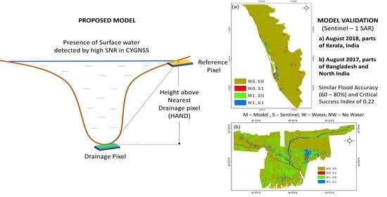Recently, this data has found land surface applications in the form of large-scale flood inundation mapping [20,21] through change detection approaches. The signals operating in the L-band penetrate clouds, and are less affected by signal attenuation through heavy rainfall and vegetation than observations in other frequencies, and thus provide an all-time and -weather observational capability. The inland areas, when submerged in water, have a distinctive increase in signal strength when compared to non-water surfaces. Water, being a smooth scatterer, reflects most of the incoming GPS signals, and hence the signals received by the 8-satellite CYGNSS constellation from a water-covered surface have enhanced signal strength. Thus, GNSS-R acts, in this case, as a dynamic indicator of the presence of water on a near-global daily scale. However, the reflected GPS data points are pseudo-randomly distributed as a function of the satellite positions, and hence the same location may not be mapped periodically, effectively resulting in a coarse daily spatial footprint for CYGNSS over land surfaces. Hence, it is hypothesized that upon integrating fine resolution static topographic information with highly frequent signal-to-noise ratio (SNR) data, it will be feasible to obtain actionable flood inundation maps that provide useful information regarding how susceptible to inundation a given region will be for a given flood event.

Height above nearest drainage (HAND) is a topography-based conceptual flood terrain index that quantifies the floodplains along the river reach into pixels, which are identified by their relative height to the nearest drainage point along the flow direction from the corresponding pixels [22,23,24]. However, it is a static flood terrain index that does not provide any information about the propagation speed of the flood wave, or if an area will be inundated or not. The index also requires a flood height cut-off, which acts as a threshold for the floodplain area, which in turn may then be used to derive the flood inundation extent. Studies have shown that there exists a large amount of overestimation of the floodplain area, depending on the threshold value chosen and the quality of the digital elevation model (DEM) used for estimating HAND values [25,26,27,28]. In addition to the HAND index, which provides information on the floodplain, further information is therefore needed to characterize the flooding potential of a channel pixel, which can be obtained by the slope of nearest drainage (SND), which is a function of the height of water in it. Thus, HAND and SND together act as static indicators for deriving flood extent, while CYGNSS provides dynamic information.

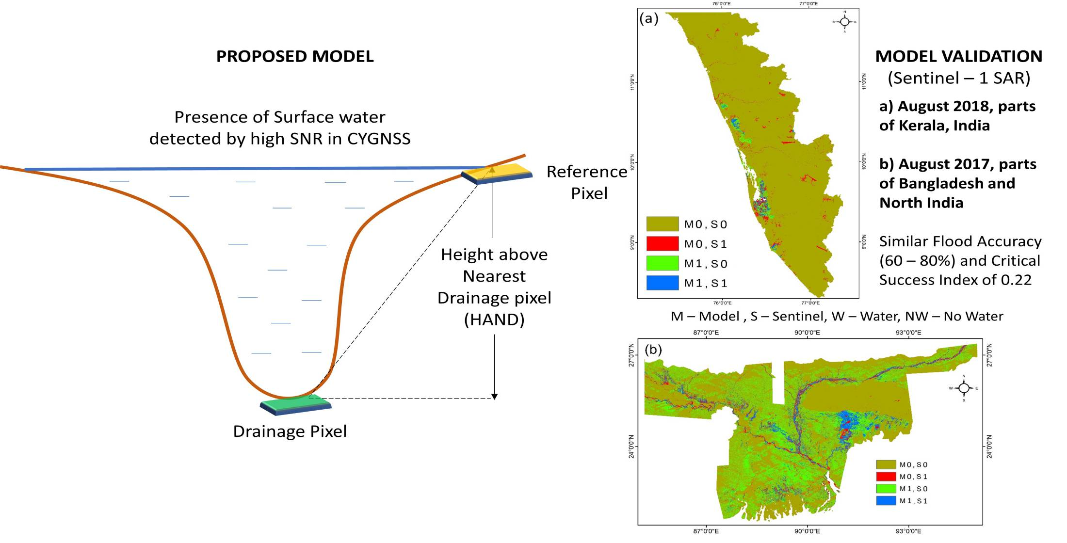
In this work, complimentary dynamic CYGNSS and static HAND-SND datasets are combined to map the extent of floodplain areas arising in the case of riverine floods. The proposed model was analyzed and compared against Sentinel-1A SAR-derived flood maps [7]. The error associated with the corresponding threshold values of the proposed method was determined. The potential of future GNSS-R-enabled satellite system missions in flood inundation mapping is also explored. The present paper is organized as follows: Section 2 describes the dataset used for model development and comparison, as well as the study area; Section 3 explains the methodology undertaken; Section 4 illustrates the results obtained and discussion therein; and finally, Section 5 provides the conclusion.

2. Data Used and Study Regions

The CYGNSS satellite constellation is an eight-satellite bi-static radar system launched by NASA in December 2016, collecting near-global (between 38°N and 38°S latitudes) daily reflected L-1 coarse acquisition (C/A) GPS signals in the form of delay-Doppler maps (DDMs), with four simultaneous point observations measured by a single satellite. The DDMs capture the behavior of the reflecting surface, characterized by the specular point of reflection and reflectivity of the surface itself, and strength of the reflected signal as indicated by the signal-to-noise ratio (SNR). For the model development, SNR data was obtained from the Level-1 bistatic radar cross-section (BRCS) of Earth surface data collection, hosted at the University of Michigan [29] (Supplementary Table S1). The globally available open-access Advanced Spaceborne Thermal Emission and Reflection Radiometer (ASTER) digital elevation model (DEM) Version 3 (GDEM 003) dataset was also used in this study, which is provided as 1° × 1° tile at 30 m spatial resolution, and referenced to the WGS84/EGM96 geoid [30]. The proposed model is applied to two regions suffering from flood events: (a) the southern Indian state of Kerala with an area of 38,000 km² (August 2018); and (b) Bangladesh and parts of North and Northeast India, including the states of Uttar Pradesh, Bihar, West Bengal, Sikkim, Assam, and Arunachal Pradesh, totaling an area of 531,000 km², which witnessed widespread and heavy flooding during the monsoon season of 2017 [31]. Both study regions are having contrasting land use/land cover, with the state of Kerala characterized by uneven, hilly terrain, while parts of North India are among the flattest delta regions in the world. This makes it prone to regular flooding, while Kerala has witnessed sporadic periods of intensive flooding. North India is also home to the most fertile basins of Ganga and Brahmaputra, because of the sedimentation following its floods. The proposed model was evaluated for its robustness over those two regions featuring contrasting topographic and flooding behaviors. Sentinel-1 synthetic aperture radar (SAR) ground range detected (GRD) imagery [32] acquired in vertical (VV) polarization during the flood events of Kerala in August 2018 and over parts of North India across August 2017 (Supplementary Table S2) was used to derive the flood inundation extent that was used for validating against the inundation extent obtained from the proposed model.

3. Methodology

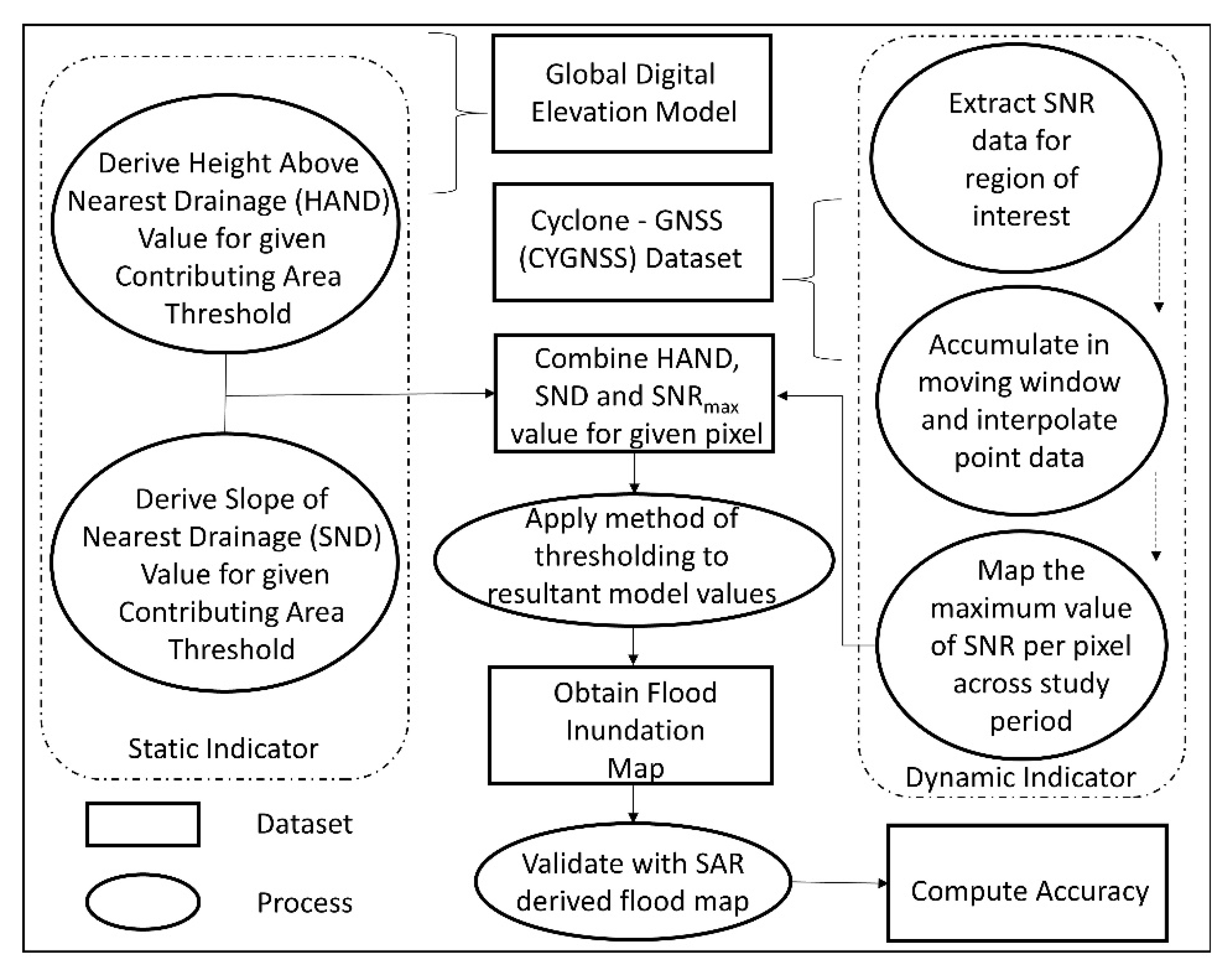
The proposed model workflow for the conceptual near-global flood inundation mapping technique is shown in Figure 1. The multi-temporal SNR data available from CYGNSS as point information, although useful in providing information regarding the underlying surface, has considerable spatial gaps in their daily ground footprint, which prevents mapping floods consistently across inland areas. Therefore, in order to obtain spatially contiguous flood inundation maps, the daily SNR point data was accumulated across a temporally moving window of 30 days length, traversing a two-month period before and during the flood event for the given region; i.e., SNR values from the (1 July to 1 August) window are used cumulatively to obtain an SNR spatial map by following the inverse distance weighted (IDW) interpolation technique, before proceeding to the next window iteration (2 July to 2 August), until the (30 July to 30 August) iteration. Extreme rainfall was observed from 1 August in both the case studies; hence the study period was considered for a total of two months, i.e., one month prior to and one month after the start of the rainfall event. The temporally moving window of a duration of roughly 30 days was taken as a baseline for mapping observed flood events of about 2-week duration. Since there existed no meaningful relationship between the semi-variance of SNR data as a function of the search radius, the value at a particular pixel was interpolated from the values of the three nearest neighboring SNR data points using IDW at 30 m spatial resolution to produce continuous surface values. The maximum value among the SNR spatial maps generated for each pixel was recorded and combined with the topographical information in the form of the HAND-SND terrain index to enhance the spatial extent of maximum inundation that can be mapped.

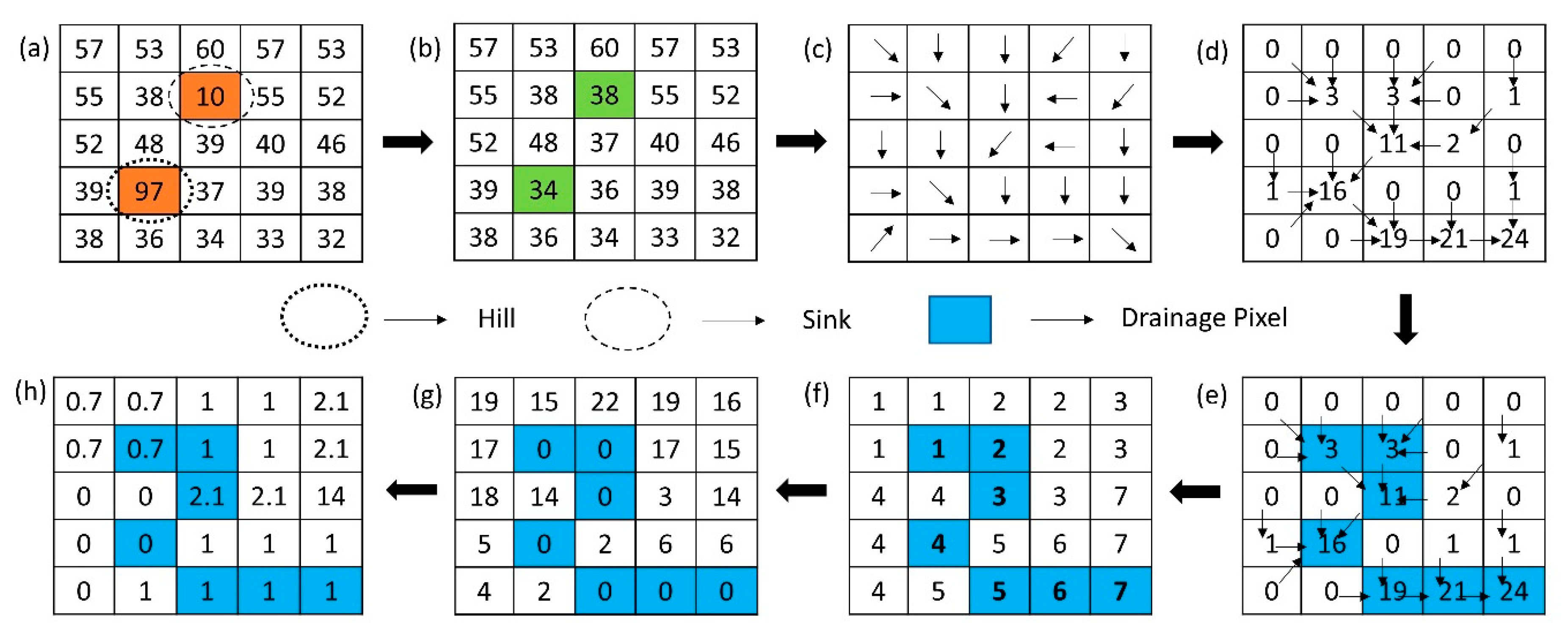
Calculation of the HAND value for a given pixel was performed as follows (Figure 2):

• ASTER DEM was filled, to avoid sinks and to make it hydrologically consistent.
• The D8 flow direction algorithm (Figure 2c) was applied to the filled DEM.
• Flow accumulation raster was obtained from flow direction, to find how many pixels drain to neighboring downstream pixels.
• Stream raster was delineated by choosing the appropriate cumulative area (CA) threshold. In this case, the CA value of 1.000 was chosen.
• Based on the flow direction raster and the stream raster delineated in the earlier step, the nearest drainage pixel for every pixel in the study area was found.
• Finally, the HAND value of a pixel at 30 m spatial resolution was calculated as the height of pixel relative to its nearest drainage pixel.

The effect of critical parameters that affect the flood extent is determined for the integration of CYGNSS and HAND-SND datasets. A flooded pixel is associated with higher SNR value, and hence the maximum SNR value mapped in the window period, w, can be assumed to have a directly proportional relationship with the likelihood of flooding P(F), where F represents the flood variable, i.e.,

P(F) ∝ Max (SNR)|_w

(1)

Furthermore, based on the HAND flood terrain model, it can be concluded that the higher the HAND value of a pixel, the less likely it is to be flooded than a pixel with a relatively lower HAND value, and hence,

$$\mathrm{P}(\mathrm{F}) \propto \frac{1}{\mathrm{HAND}}$$

(2)

Similarly, once we have the nearest drainage map derived from step 5 mentioned above, the slope of the nearest drainage (SND) is then assigned to its corresponding floodplain pixel (Figure 2h). This step was performed because drainage pixels with the same HAND value and nearest channel pixels with higher slope values are less likely to inundate than those drainage pixels with lower slope values. Also, Manning’s Equation shows that a given discharge amount ($Q$) in the channel is proportional to hydraulic radius ($R$) and channel slope $\left(S\right)$, where $Q\propto R^{5/3}{S}^{1/2}$. Furthermore, for wide rectangular channels, ($B\gg H$) $R$ simplifies to ${BH}^{5/3}$, where $B$ is the channel width and $H$ is the discharge height. If the value of $B/\mathsf{\eta }$ is assumed constant (where $\mathsf{\eta }$ denotes the roughness coefficient of the riverbed), it can be concluded that for a given discharge, the water level in the stream is inversely related to the slope of channel pixel given as $H\propto S^{-3/10}$, and therefore,

$$\mathrm{P}(\mathrm{F}) \propto \frac{1}{{\mathrm{SND}}^{0.3}}$$

(3)

In order to characterize the static potential of flooding, the following points are required: (a) the height of a given pixel relative to the nearest drainage pixel height; and (b) the height of the water level in the channel, which is inversely related to the slope of the channel pixel, as shown above. This characterization is in contrast to [24], which considers the slope of a floodplain pixel relative to the nearest drainage pixel as an extension of HAND. Thus, combining (1), (2), and (3), the dynamic (CYGNSS) and static (HAND and SND) dataset available for the study region under consideration was formalized as follows:

$$\mathrm{P}(\mathrm{F}) \propto \frac{{\mathrm{MAX}\left(\mathrm{SNR}\right)|}_{\mathrm{w}}}{(\mathrm{HAND}\times {\mathrm{SND}}^{0.3})}$$

(4)

The product of HAND and SND can result in null values in the case of pixels located within channels, leading to undefined model output. We consider that 1 + (HAND × SND^0.3) ≅ (HAND × SND^0.3), and thus the model variable F from (4) was further simplified without considering any additional parameters in the following form:

$$\mathrm{F} = \frac{{\mathrm{MAX}\left(\mathrm{SNR}\right)|}_{\mathrm{w}}}{1+(\mathrm{HAND}\times {\mathrm{SND}}^{0.3})}$$

(5)

In addition, the proposed model output raster was subjected to different model output threshold values to obtain the respective maximum extent of inundation across the flood duration at 30 m resolution. The model was compared against co-located Sentinel-1 GRD VV-polarized images. Those images were pre-processed by applying standard steps, including (a) applying the orbit file; (b) sub-setting of the images; (c) thermal noise removal; (d) border noise removal; (e) radiometric calibration; (f) speckle filtering using a Lee filter of 7 × 7 window size; and (g) range-Doppler terrain correction, followed by image binarization using Otsu’s method [33]. The model sensitivity analysis was performed by introducing parameter β to (5), yielding

$$\mathrm{F} = \frac{{\mathrm{MAX}\left(\mathrm{SNR}\right)|}_{\mathrm{w}}}{1+{(\mathrm{HAND}\times {\mathrm{SND}}^{0.3})}^{\mathsf{\beta }}}$$

(6)

and analyzing the flood accuracy (FA) and critical success index (CSI) parameters for different threshold values. These parameters are given by

$$\mathrm{FA} = \frac{\mathrm{h}}{\mathrm{h}+\mathrm{m}}$$

(7)

$$\mathrm{CSI} = \frac{\mathrm{h}}{\mathrm{h}+\mathrm{m}+\mathrm{z}}$$

(8)

where h represents the number of pixels which have an agreement (hit) between model and reference pixels, m represents the number of pixels that the model has failed (miss) to identify as inundated when compared with the reference inundation map, and z represents the number of pixels that the model has overestimated as inundated when compared to the reference.

4. Results and Discussion

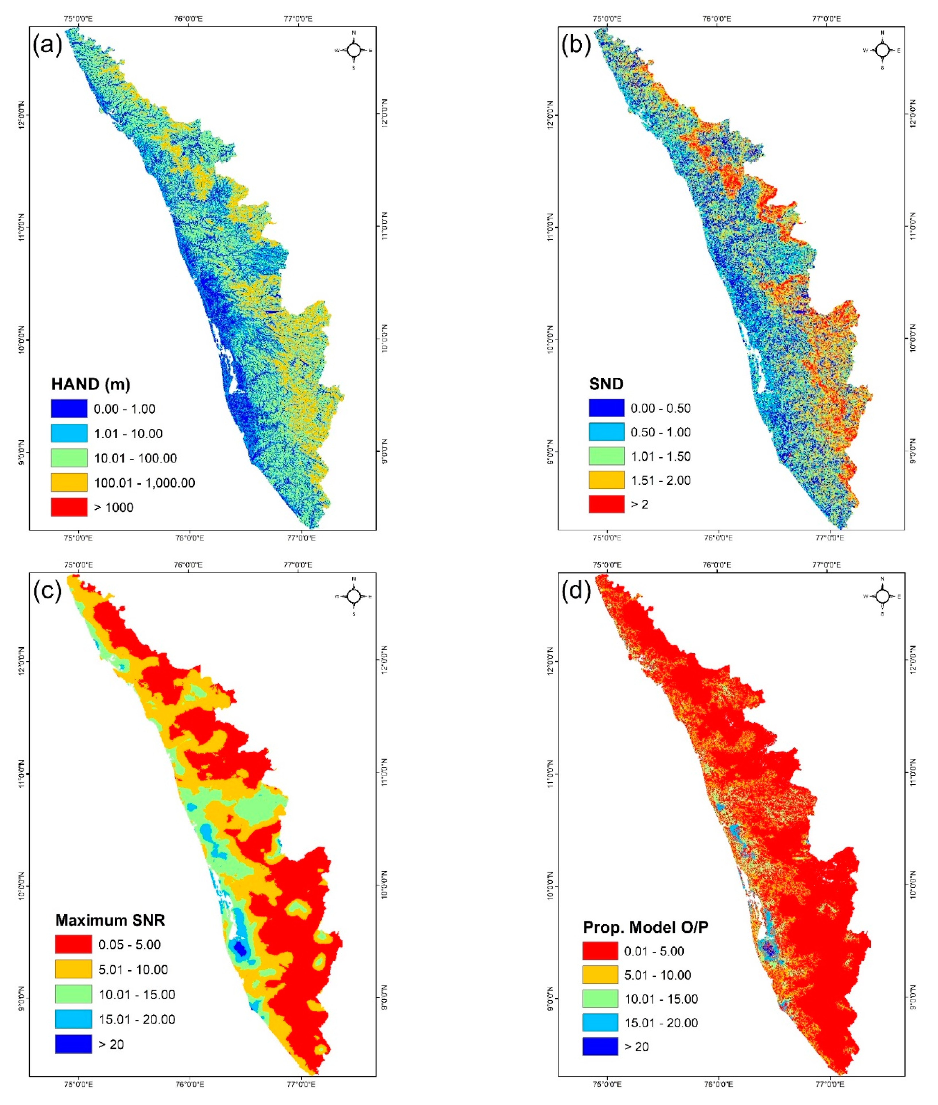
After processing the ASTER DEM, the HAND flood terrain model for Kerala was obtained, as shown in Figure 3a. The figure shows that Kerala is enveloped by the mountainous Western Ghats to the East, which is associated with high HAND and SND values (Figure 3b), and the relatively flat flood plains along the east coast on the left. The CYGNSS Level-1 BRCS SNR daily data was extracted over the southern Indian state of Kerala for the August 2018 flood event, accumulated across the 30-day window period before and after the flood event and spatially interpolated, yielding the maximum SNR values, as shown in Figure 3c. The coastal areas are clearly associated with higher SNR values than the mountainous Western Ghats. These values are indicative of surface water present in the pixel and coincide with ground observations of flood points reported at the time [34]. However, the SNR data alone cannot accurately map the inundation at the river channel scale, because of the mixed pixel response from the water surface along the coastlines. It can only provide overall information on which places could have been inundated across a large spatial extent of the study region. Hence, the proposed merged model output from CYGNSS, HAND, and SND data yields possible inundation, as shown in Figure 3d. 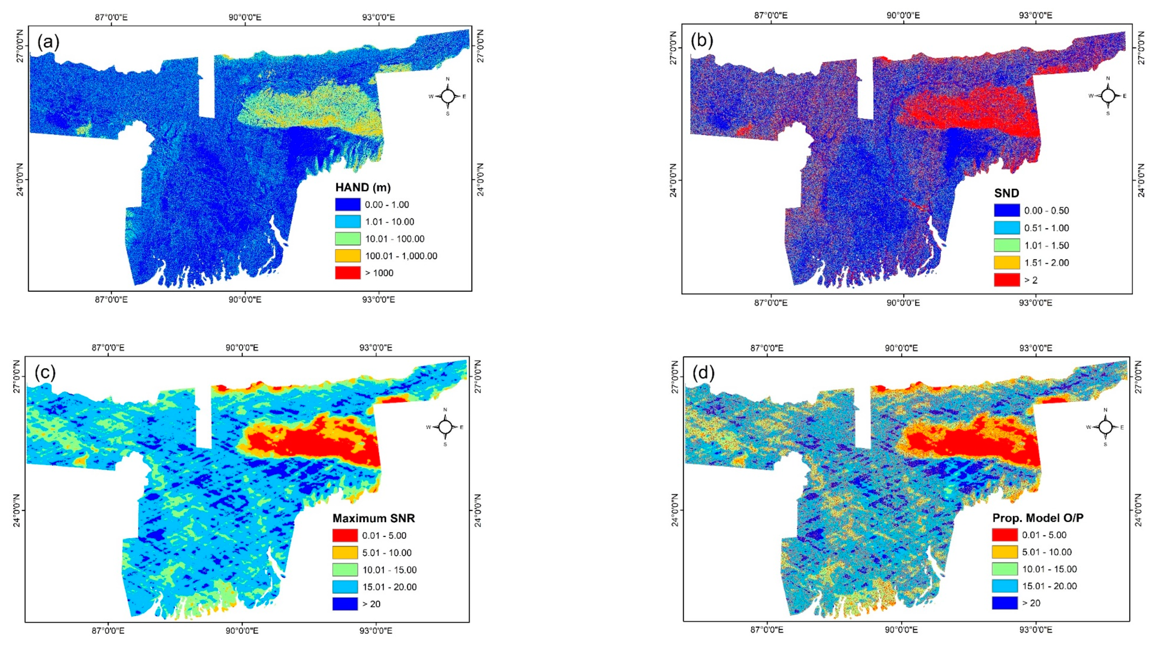The model output indicates areas that have higher values in the low-lying parts of the central and southern coastal areas, which witnessed extensive flooding [34]. In the case of the August 2017 flood event across North India and its neighboring regions, most of the terrain, except the mountainous Arunachal Pradesh, is flat, and associated with low HAND (Figure 4a) and SND (Figure 4b) values across the floodplains of the Ganga and Brahmaputra rivers, making it prone to extensive flooding. The processed CYGNSS data indicates large areas with significant SNR values (<15) across the study region, as shown in Figure 4c. The combined output also shows a significant increase in model value across large portions of the floodplain areas, given in Figure 4d. It must be noted that HAND, and SND as its extension, were chosen based on a better conceptual representation of hydrologic similarity of floodplain regions than other topographic indices [35].

In the case of the Kerala flood event, Sentinel-1A could capture the flood inundation only on August 21, 2018, and hence imagery available (three scenes) over parts of Kerala state was used for deriving inundation extent by thresholding the pre-processed SAR image using Otsu’s method of binarization. The inundation extent was derived at 30 m spatial resolution (shown in Figure 5a) to make it comparable with the proposed model result. The reference inundation map exhibits a similar inundation pattern, as shown by the model output inundation extent.

The model output was then subjected to different threshold values, to compare how the extent of inundation matched with the validation inundation map obtained from SAR imagery. Figure 5b shows the maximum extent of inundation obtained after considering a model output threshold value of 15 overlaid with the validation inundation map with the percentage overlap of flooded and non-flooded areas, as well as the over- and underestimation by the proposed model indicated. 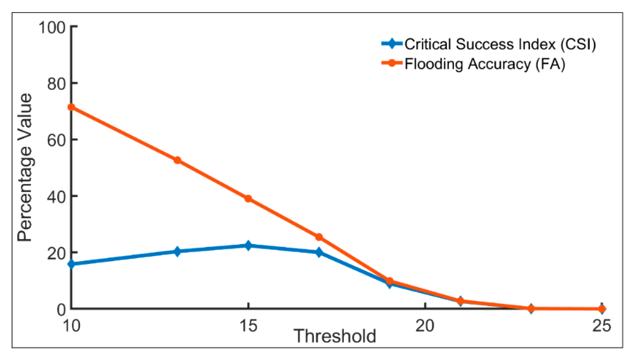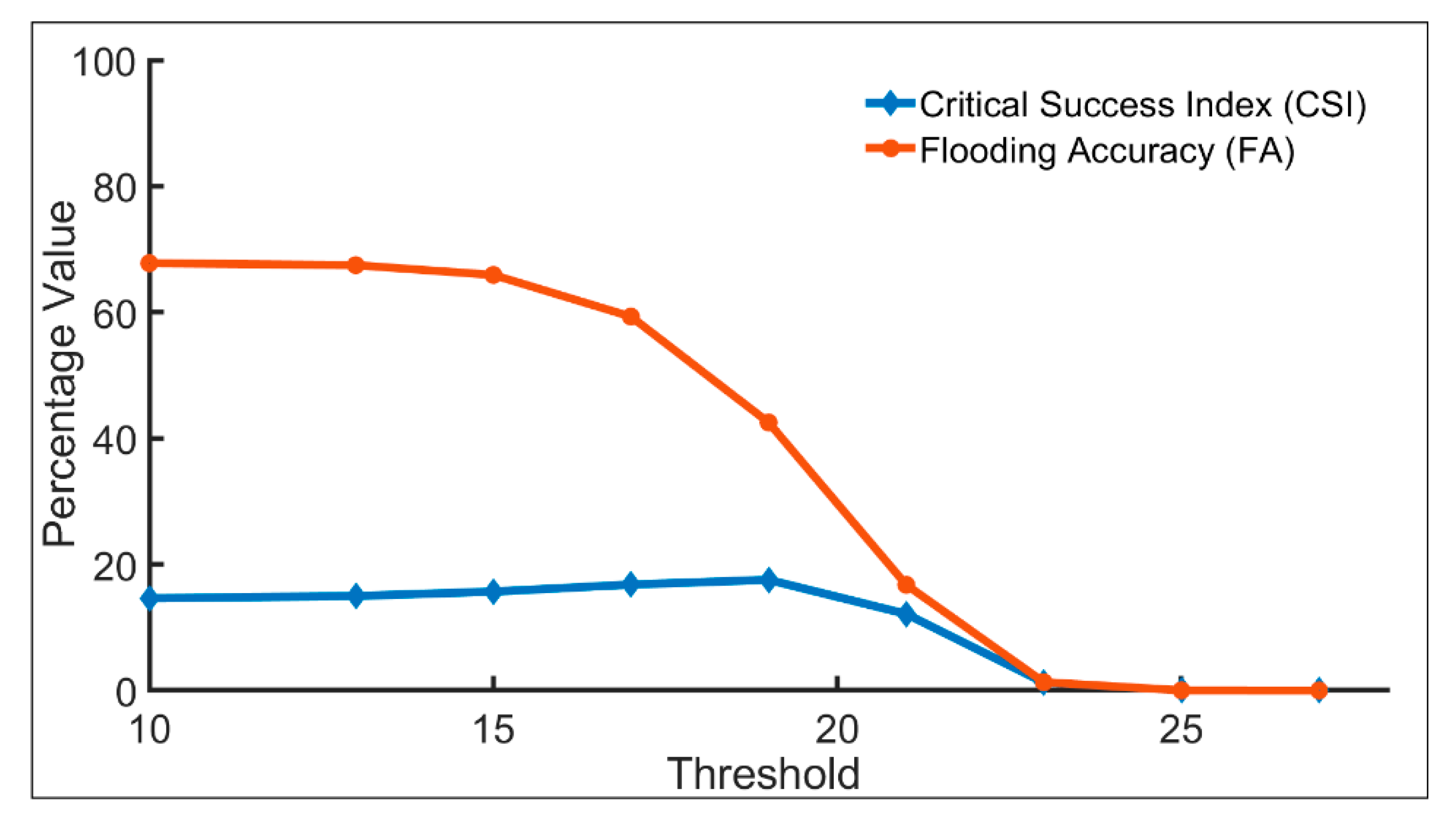Figure 6 shows the variation of the CSI calculated (from (7)) between both the inundation maps with the threshold value.

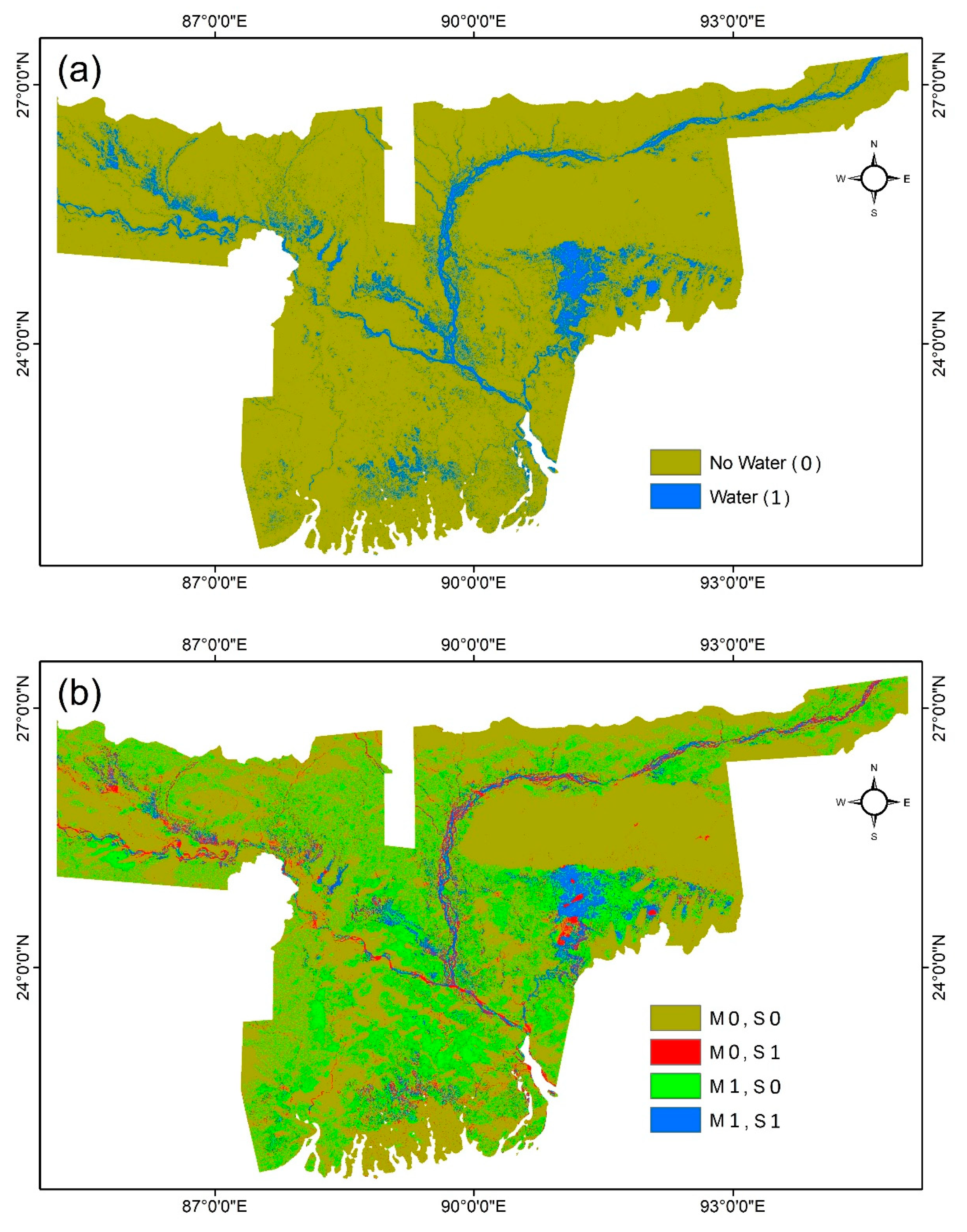
The model results were found to be most sensitive around values of 15–19, after which FA and CSI decreased considerably. For lower values of model threshold, high values of FA were observed, but the corresponding value of CSI indicates the presence of model overestimation. In the case of the North India flood event of August 2017, several Sentinel-1 SAR scenes were collected across different days (24–29 August) of the flood period, subjected to thresholding, and mosaicked to obtain a rough extent of inundation across such a large study region (Figure 7a).

Similar to the case of the flood event in Kerala, the model output was subjected to thresholding for different values. The overlapped inundation map obtained for a sample threshold value of 15 with the reference inundation map from Sentinel-1 SAR shows that there exists a large amount of overestimation error by the model (Figure 7b). This overestimation by the model was found to be mainly caused by:

• Coarse spatial resolution of the CYGNSS SNR points, which are spaced widely apart, whose signal strength also depends spatially on the first Fresnel zone of the coherently reflecting surface.
• Poor vertical accuracy and coarse spatial resolution of the ASTER DEM in resolving the floodplain areas, which caused the HAND flood terrain model being unable to distinguish between the river channel and the delta regions.
• Sentinel-1 SAR imagery suffering from larger temporal latency and therefore failing to capture the maximum inundation, which will be complemented by the daily available CYGNSS dataset.
• Presence of many irrigated paddy fields in the fertile area of the Ganga and Brahmaputra delta region, as well as the presence of dense vegetation in the case of Kerala, can result in the proposed model identifying those high-moisture regions as being inundated due to flood event.

Also, Figure 8 underlines that the model result was sensitive around 17–21, much as the earlier CSI plot obtained for the Kerala flood event. At higher threshold model values (>20), substantial underestimation errors in inundation mapping exist, which shows that the proposed model was highly sensitive around model values of 17–19 when considering both cases.

However, the model threshold value cannot definitively be fixed for a given flood event to obtain the flooding extent, because of the varied land-use/land-cover usage (including interference due to non-flooding attributes in the case of inundated paddy fields dominating the North India study region) and flooding behaviors associated with the study regions. Furthermore, the model structure was modified by including an exponential parameter, β, to the static (HAND and SND) part of the term which was varied from 0.1 to 10, resulting in similar CSI values for a given model threshold value for both the cases. This insensitivity to model structure variation is due to the over-/underestimation of the inundation extent as obtained by the HAND/SND threshold, as this is more sensitive to the channel initiation value (contributing area) [27] than assigning more/less weight to the HAND/SND values in itself.

This model was applied to flood events arising due to extreme rainfall events, and specifically, the SND component is applicable only in case of floods arising with respect to channel pixel slope values. The model cannot be applied in its current form to other forms of flooding, including pluvial or coastal flooding, which can be possible only by considering other relevant factors.

As such, there are several limitations to the validation of the proposed model. These include the choice of Sentinel-1A SAR data as the only other reliable source that can provide the spatial extent of a flood inundation. However, the Sentinel satellite overpass over the study regions was mostly during the receding phase of both the flood events; hence the flood peak extent could have probably been missed. Furthermore, the FA and CSI values are also affected by the amount of observational overlap between CYGNSS and Sentinel-1 datasets, as they do not have the same coverage extent and daily repeat rates. The presence of vegetation in both study regions greatly affects the accuracy in deriving the flood extent from SAR images, while rain and wind also affect the omission of inundation retrievals from single SAR imagery. In addition, the presence of smooth surfaces in the reference scene, including roads and rooftops, cause commission errors [36].

In the future, by adopting a probabilistic framework [37], through which it will be possible to generate a probabilistic flood inundation map by exploiting the histogram of the combined model output and separating the non-water pixels, which will result in better mapping capabilities of the inundation uncertainty for a region. With the availability of additional improved GNSS-R SNR datasets, from other navigation satellite constellations, there are active navigation signals that are already available, which are sensitive to the presence of inland surface water that can have downstream applications [38], including inundation mapping in the case of flood events. Those include satellites operated by different space agencies around the world, such as the Global Navigation Satellite System (GLONASS) of Russia), European Space Agency’s GALILEO, and the Navigation with Indian Constellation (NavIC), launched by the Indian Space Research Organisation (ISRO).

5. Conclusions

GNSS-R Signals of Opportunity (SOOP) are sensitive to the presence of surface water. The study proceeded, considering these signals to be highly temporal (sub-daily); however, because of the poor spatial resolution (order of kilometers) available for a given region from CYGNSS [39], SNR data points were accumulated and interpolated spatially, employing a moving window approach before and during a flood event. The maximum observed SNR value during the flooding period provides an opportunity to estimate the maximum flood inundation extent while integrating those with topographical information. Thus, this paper explored the potential of combining the coarse resolution, but temporally dynamic, GNSS–R signals with the static, but spatially continuous, HAND-SND-based flood terrain index for high-resolution global flood inundation mapping. CYGNSS SNR daily data was extracted for two flood events, one over the southern Indian state of Kerala during August 2018, and for an extensive event during August 2017 across Bangladesh and parts of North and Northeast India. HAND and SND values were calculated for the respective study regions and were integrated with CYGNSS SNR data using the proposed approach. The model was evaluated with flood inundation maps derived from Sentinel-1 SAR imagery available during the flood duration. It was found that the model-derived inundation extent was sensitive to values around 17–19 on thresholding with a maximum CSI of 0.22, although there was high flooding accuracy (FA) in mapping 60–80% of flood extent for lower model threshold values. The significant over-/underestimation is mainly attributed to the spatially-coarse pseudo-randomly distributed SNR data, and to the limited availability of the Sentinel-1 SAR imagery. This method thus gives an advantage over existing SAR satellite-derived flood inundation methods, because (a) SAR-derived flood maps provide only an incomplete snapshot, not covering the entire extent of flooding, whereas in the case of CYGNSS, a near-global daily coverage is available; and (b) because of low revisit frequency in the case of SAR satellites, they are not able to provide information about the spatial dynamics of the flood event. Thus, there exists no single standard dataset which can satisfy all the conditions that are necessary for the temporal evolution of flood inundation extent to be captured with reasonable accuracy. With a larger amount of GNSS–R data available in the future, this approach provides an opportunity that would greatly benefit peak flood extent estimation, and also help in mapping floods at the sub-daily temporal resolution, which can provide useful information when a flood intensifies and recedes.