Article

Thermography as a Tool to Assess Inter-Cultivar Variability in Garlic Performance along Variations of Soil Water Availability

by
Álvaro Sánchez-Virosta
* and
David Sánchez-Gómez
Instituto Regional de Investigación y Desarrollo Agroalimentario y Forestal de Castilla La Mancha (IRIAF), CIAF de Albaladejito (Cuenca, Spain), Ctra-Cuenca-Toledo, km. 174, 16194 Cuenca, Spain
*
Author to whom correspondence should be addressed.
Remote Sens. 2020, 12(18), 2990; https://doi.org/10.3390/rs12182990
Submission received: 5 August 2020 / Revised: 4 September 2020 / Accepted: 13 September 2020 / Published: 14 September 2020
(This article belongs to the Section Remote Sensing in Agriculture and Vegetation)

Abstract

:
Climate change entails increasingly frequent, longer, and more severe droughts, especially in some regions, such as the Mediterranean region. Under these water scarcity conditions, agricultural yields of important crops, such as garlic, are threatened. Finding better adapted cultivars to low water availability environments could help mitigate the negative agricultural and economic impacts of climate change. For this purpose, plant phenotyping protocols based on remote-sensing technologies, such as thermal imaging, can be particularly valuable since they facilitate screening and selection of germplasm in a cost-effective manner, covering a wide range of temporal and spatial scales. In this study, the use of a thermal index known as the crop water stress index (CWSI) was tested as a predictor of bulb biomass and for the assessment of inter-cultivar variability of five garlic cultivars in response to a gradient of soil volumetric water contents (VWCs). Three experimental assays, one in the 2018 season and two in 2019, covering a wide range of water availability levels were carried out. Different linear models were developed, with CWSI and VWCs as continuous predictors of bulb biomass, and the factor cultivar as a categorical predictor. The results support the existence of inter-cultivar variation in terms of sensitivity to water availability. The most productive cultivars under favorable conditions were also the most sensitive to water availability. In contrast, the cultivars with lower bulb production potential displayed lower sensitivity to water availability and higher stability across experimental assays. The results also support that CWSI, which was sensitive to inter-cultivar variability, is a good predictor of garlic bulb biomass. Therefore, CWSI can be a valuable tool for garlic phenotyping and cultivar screening.

1. Introduction

Erratic climatic conditions brought about by climate change entail a great instability in crop yields throughout crop seasons [1,2,3], which causes economic losses [4]. These economic and yield damages could be buffered with more resilient agroecosystems based on crop biodiversity [5,6]. In this sense, finding sustainable, resilient, and more yield-stable cultivars under different environmental conditions becomes crucial, especially under climate change scenarios [7,8,9,10,11].
Crop phenotyping is currently in the search for improved genotypes/cultivars against abiotic and biotic stresses [12,13]. Thus, intraspecific characterization of functional and yield responses to the environment should be a key approach in crop breeding and selection programs [14]. For this purpose, crop phenotyping and cultivar selection must be performed in a cost-effective manner with practical implementation [15,16,17]. In this sense, the use of new technologies, along with enhanced agro-biodiversity, represents a host of promising opportunities to improve agriculture sustainability and crop adaptability to climate change [18,19,20].
Plant phenotyping based on rapid, scalable, and non-invasive techniques could optimize the assessment of inter-cultivar or inter-genotype variability in the plant response to the environment [16,18]. Remote-sensing techniques along with functional plant modelling allows for the assessment and analysis of key functional traits in a wide range of temporal and spatial scales [18,21,22]. In this sense, certain thermal indices derived from infrared thermal imaging, such as the crop water stress index (CWSI), have been reported as effective and useful tools for plant phenotyping, regarding plant water relations in response to environmental conditions [23,24]. Since the introduction of CWSI by Idso et al. [25] and Jackson et al. [26], this index has been progressively used as a proxy for stomatal conductance and transpiration with practical applications (see [27] and references therein). For example, it has been successfully applied for inter-cultivar drought-tolerance screening in lentil [28] and grapevine [29] and for irrigation scheduling in cotton [30] and potato [31]. However, to the best of our knowledge, the use of thermal imaging has not been explored in other important horticultural crops, such as garlic.
Garlic (Allium sativum. L) ranks second among the most cultivated Allium crops worldwide, with a steadily increasing global production that reached 28.5 million tons (mt) in 2018 [32]. Particularly in the Mediterranean region, garlic is a widely distributed crop [33], being an important element of the Mediterranean diet and considered as a functional food because of its bioactive components [34,35]. However, the high sensitivity of bulb formation to environmental factors (e.g., water deficit, high temperatures, etc.) is threatening this important crop in the current context of climate change [36,37,38]. The Mediterranean climate is characterized by a great seasonal and inter-annual variability, with dry periods and a high frequency of droughts and heat waves. Moreover, extreme climatic events have been more frequent in the last decades and are expected to increase in the Mediterranean region [39,40]. This induces an additional stress for current and future irrigation resources of the region [41,42].
Garlic crop improvement and adaptation is crucial under these climatic scenarios. However, breeding of garlic is limited by the fact that the majority of cultivars are non-fertile and very specific conditions are needed for florogenesis and seed production [43,44]. In this context, the assessment and understanding of inter-cultivar variability of garlic in response to stressful environmental conditions, and the selection of the already existing genotypes, is crucial for its adaptation to future environmental conditions linked to climate changes [45]. Some attempts have been made to conduct cultivar screening and phenotyping in garlic [46,47,48] and to assess growth and/or bulb production variation in response to environmental conditions [38,49,50]. However, the assessment of inter-cultivar variation in response to water availability [51] is still scarce. In this regard, the need to include inter-cultivar variability in plant growth and yield response models to environmental conditions has been highlighted. It will improve efficiency in maximizing yields and develop effective mitigation and adaptations tools in garlic [49].
The objective of this study was to evaluate a stress index (CWSI) based on a non-invasive methodology, such as thermal imaging, to be implemented on garlic crop management. Specifically, CWSI was evaluated as a potential valuable index able to assess inter-cultivar variability in bulb production in response to a gradient of soil moisture. Different linear models were performed where two continuous predictors (Cp) of bulb production, CWSI and soil volumetric water content (VWCs), alone or in combination, and the categorical factor cultivar were evaluated. These models were tested to determine the variability in the response of five garlic cultivars to a gradient of VWCs across three experimental assays, one in 2018 and two in 2019, in two different locations and different weather conditions.

2. Materials and Methods

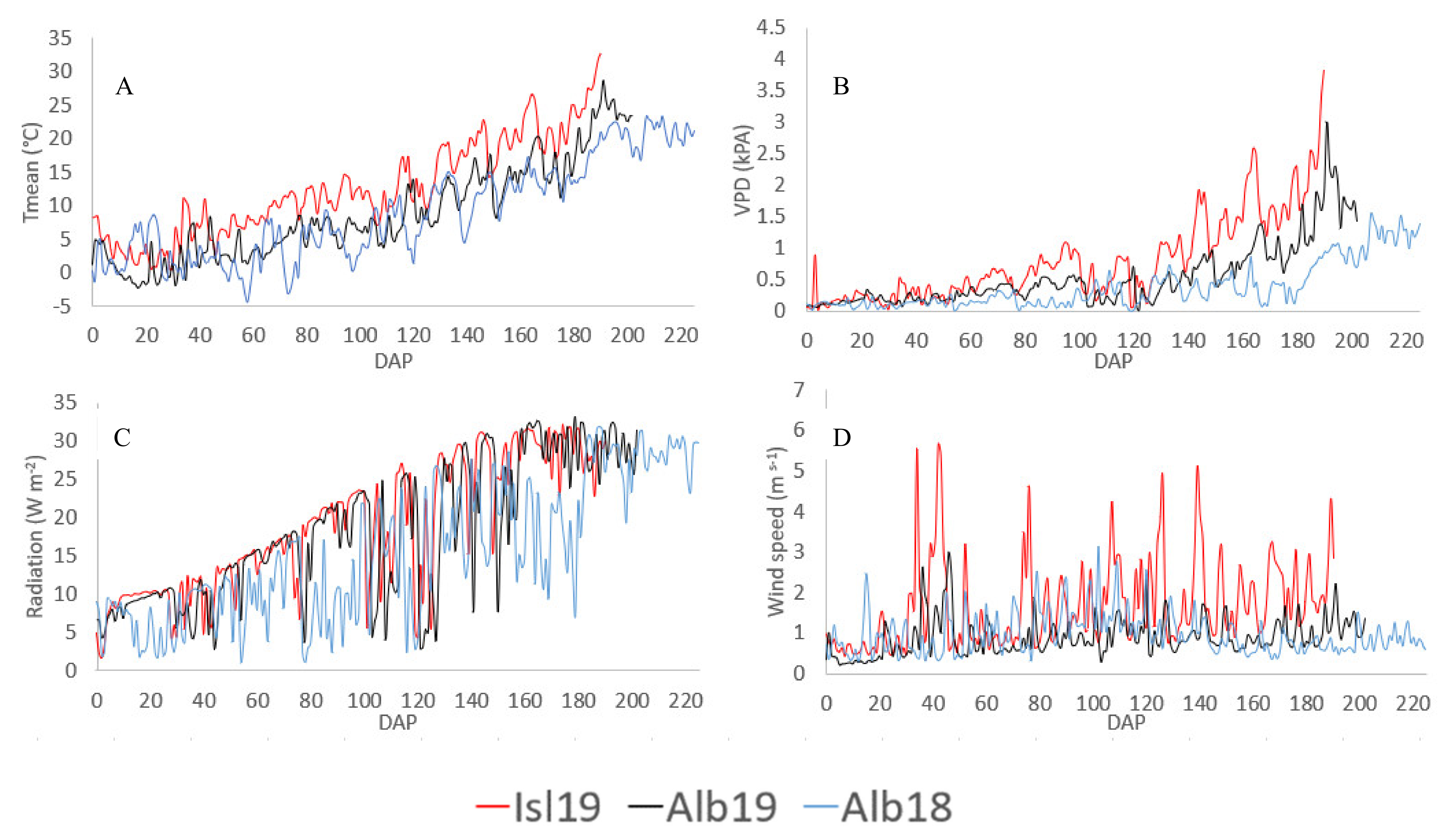
2.1. Study Site and Weather Conditions

Three field assays were carried out during two consecutive seasons, 2017–2018 and 2018–2019 (hereafter referred as “2018” and “2019”, respectively). During 2018, we conducted one of the assays (Alb18) at the “Centro de Investigación Agroforestal de Albaladejito” (40°04′31.436N, 2°12′18.061W, altitude 902 m.a.s.l) in Cuenca, inland Spain. The climate of this region is classified as a Mediterranean-continental climate, characterized by cold winters (mean minimum temperature) and hot and dry summers, with strong thermal oscillations with mean (minimum–maximum) temperatures of −1.5 °C in January to 30.1 °C in July [52]. Historical average annual precipitation and temperature are ca. 500 mm and 11.8 °C, respectively [52]. The soil of Albaladejito is a sandy silt loam. For additional details of its physicochemical characteristics, see [53].
In 2019, two additional assays were placed in two locations. The first one was placed at Albaladejito (Alb19) in an experimental plot close to that of Alb18, and the other one (Isl19) was placed at IMIDRA’s experimental station, “La Isla” (40°18.75′N; 3° 29.89′W; 528 m.a.s.l), in Arganda del Rey, Community of Madrid, 140 km away from Albaladejito. “La Isla” is located in the central region of the Iberian Peninsula, within the domain of the Mediterranean-temperate climate, with a Mediterranean-continental tendency. Historical average annual rainfall is between 440 and 490 mm and the average annual temperature is around 13.8 °C [52]. The soil in “La Isla” is a sandy silt loam with the following chemical characteristics: pH of 8.5; 1.3% organic matter; and 0.3% nitrogen, 42 mg phosphorus (P)/kg, and 434 mg potassium (K)/kg. Soil analyses were performed by “Laboratorio de Suelos IMIDRA” (Instituto Madrileño de Investigación y Desarrollo Rural, Agrario y Alimentario, Madrid, Spain). Soil analyses were carried out before the establishment of the assay, but determinations from previous years show very constant inter-annual values.
Meteorological data at Albaladejito were recorded with a micro-meteorological station, Vantage pro 2 model 6152EU, Davis Instruments, Diablo, US, in 2018 and 2019. At “La Isla” these data were collected from a weather station placed in the experimental farm named “Arganda”, which belongs to the national network of the agroclimatic information system for irrigation, managed by the MAPA (http://eportal.mapa.gob.es/websiar/Inicio.aspx). Mean temperatures (Tmean), sun radiation, wind speed, and vapor pressure deficit (VPD) varied across seasons and locations. Relatively mild weather conditions were recorded in Alb18 while more severe climatic conditions were recorded in the assays of 2019, especially in Isl19 (Figure 1).

2.2. Plant Material, Experimental Design, and Watering Treatment

The five studied cultivars were selected according to their different genetic background and different origins with contrasted climatic conditions (Table 1). The studied cultivars were “Gardacho”, GAR (introduced “American type” commercial cultivar); “Purple of “Pedroñeras”, PED (popular and appreciated cultivar from Castile-La Mancha recognized by the European Union as a Protected Geographical Indication, PGI); “Fino de Chinchón”, CHI (traditional cultivar from the south of Madrid); Cbt00089, DRYII (traditional cultivar from Tenerife Island); and Port07990, RAIN (traditional cultivar from the north-west of Portugal). The bulbs for the experiment were obtained from the Bank of Plant Germplasm of IMIDRA (FAO code ESP198), the garlic cooperatives (“San Isidro el Santo” and “Coopaman S.C.L”, “Las Pedroñeras”, Cuenca, Spain), the Agricultural Biodiversity Conservation Centre of Tenerife (CCBAT), and the Portuguese Bank of Plant Germplasm.
The five garlic cultivars were planted on field plots across a gradient of soil water availability. In Alb18, 4 cloves of each of the five cultivars were planted within 11 plots. In Alb19 and Isl19, three cloves x cultivar were planted within nine plots at each location. Before planting, the cloves were treated with 1.5% sodium hypochlorite and the fungicide Prelude (prochloraz 20%, BASF SE, Ludwigshafen am Rhein, Germany). The biggest and healthiest cloves of each cultivar were selected and manually planted within each plot. The distance between plants within a line was 0.15 m and the distance between lines was 0.40 m. The cloves were randomly placed within each plot and watered after planting to help plant establishment.
The plots were watered when needed to maintain the soil volumetric water content (VWCs) within the pre-stablished target range (Table 2). In 2019, to reach lower VWCs, the plots were covered with rainfall cover structures during rain events to avoid uncontrolled water supply. VWCs was measured at hourly intervals with FDR probes (ECH2O EC-5, Meter group, Inc., Pullman, WA, USA) connected to dataloggers (Em50, Meter group, Inc., Pullman, WA, USA) on each plot during the whole crop cycle.

2.3. Crop Water Stress Index (CWSI), Bulb Biomass, and Bulb Diameter Measurement

Ground-based thermal images (Fluke Ti300 camera, Fluke Corporation, USA, 7.5–14 μm, 240 × 180 pixels, ε = 0.96) were taken to remotely assess leaves’ temperature. The procedure described by Jones [54] was followed to include reference surfaces. Leaf references were attached to a cork board, where the ‘wet’ reference (Twet) was obtained by spraying fresh water on two detached garlic leaves while the ‘dry’ reference (Tdry) was obtained by coating detached garlic leaves with petroleum jelly. Zenithal thermal images, at a 1-m distance from the canopy, were taken so that they covered the whole plant and surface references. Thermal images were taken for every plant within each plot at least two (Alb18) or three times (Alb19 and Isl19). All the measurements were carried out throughout the bulbing phase [55]. The measurement interval was based on the growth development of each assay. The first infrared images were taken when most of the plants reached ca. 7–8 leaves while the second and third infrared images were taken when the plants achieved the peak of growth (ca. 10–14 leaves). Finally, the software, SmartView (Fluke Smartview 4.3, Fluke Corporation, Everett, WA, USA), was used for the analysis of the thermal images. To reduce the sensitivity of the analysis to variation in the leaf angles, average leaf temperatures were calculated by selecting representative areas of the youngest fully expanded leaves (Tleaf) and references using the function polygon markers of the software SmartView (Figure 2). The mean ± S.D of these Tdry and Twet references for the whole experiment were 34.8 ± 4.4 °C and 20.1 ± 3.5 °C respectively.
Finally, processed data were used to calculate the crop water stress index (CWSI) as:
C W S I = T l e a f T w e t T d r y T w e t
Bulbs were harvested at the end of the growth cycle, when the three youngest leaves were dry. Afterwards, bulbs were stored in a ventilated warehouse and weighed until constant weight to the nearest mg. At the same time, bulb diameter was measured with a caliper.

2.4. Statistical Analysis

At the end of each growing season, the VWCs data recorded on the dataloggers were collected and the integrated VWCs over the whole period for each plot were calculated using a macro (‘area below curves’) implemented in SigmaPlot 11.0 (Systat Software Inc., San Jose, CA, USA). Then, the average VWCs per day was calculated as the ratio between the area below the curve of VWCs and the number of days measured on each plot. The representative CWSI value used in the models was calculated as the average of CWSI measurements for each cultivar within the same plot. The representative bulb biomass used in the models was calculated, similarly, as the average bulb biomass of cultivar replicates on each plot. Regression linear models were used to test for the fixed effects of the continuous predictors VWCs per day and CWSI, and the categorical factor cultivar on bulb biomass. In addition to the main effects of these variables, the interaction term between cultivar and VWCs and/or CWSI were also included. Shapiro–Wilk’s, Breusch–Pagan, and variance inflation factor tests were used to test for normality, homogeneity of variances, and multicollinearity, respectively. Bulb biomass was log-transformed to meet the assumptions of normality and homoscedasticity. Additional mixed linear regression models were fitted to test for the effects of the random factor (assay). ANOVA analyses were also performed to test for the significance of the regression coefficients and to test for differences between assays. Based on the predictions of the best model, estimated marginal means of bulb biomass were plotted across selected levels of the continuous predictors and Tukey test comparisons of the slopes among cultivars were computed to identify homogeneous groups. All the models and subsequent analyses were performed using R (version 1.2.5019; RStudio Team, 2019).

3. Results and Discussion

3.1. Models’ Verification and Variable Reliability as Bulb Biomass Predictors

Alternative models differing in complexity and the number of factors were evaluated (see Table 3). The simplest models were those with only one of the continuous predictors (Cp) included, VWCs or CWSI. Both variables have been previously reported as predictors of yield and biomass gain in other crops [56,57,58,59]. The results of this study confirm that bulb biomass of garlic was positively correlated with VWCs while negatively correlated with CWSI (Supplementary Materials Table S1), with both Cp being significant (Table 4). The lower the soil water availability, the lower the bulb biomass, as displayed in previous studies in garlic [37,53,60].
The categorical factor cultivar was also significant and improved the goodness of fit and the variance explained (see AIC and R2adj of model 2 in comparison with model 1, Table 4). These results confirm the existence of significant inter-cultivar variability in garlic and agrees with the idea that the inclusion of genotypic variability in crop modeling improves the prediction of the crop response to environmental conditions [61,62,63]. The interaction between cultivar and each of the Cp were further tested in more complex models (models 3 to 5). The inclusion of the interaction terms also improved the goodness of fit and the variance explained by the models (Table 4). Taking into account the interaction between factors is important and should not be neglected. For example, when breeding programs take into account these interactions, they can lead to significantly higher crop yields [64].
Model 4, which included both continuous predictors and the interaction of cultivar with either of them, improved the AIC and R2adj, resulting in the best models tested. Additional linear mixed models including the random factor assay (model 5 in Table 3) did not improve these models (see model 5 in Table 4). Despite CWSI usually being highly correlated with water availability variables, such as volumetric water content and evapotranspiration coefficients [30,65,66], in this study, none of the models that included both predictors showed multicollinearity (variance inflation factor test). Besides, the increased goodness of fit and explained variance of the models that included both predictors in comparison with those models that included only one of the predictors suggest that CWSI accounts for a significant portion of variability that VWCs cannot explain. Moreover, the Model4Cult*CWSI, which also included the interaction of cultivar with CWSI, resulted in the best fit. CWSI is tightly related with leaf/stem water potential [67,68,69], which has been found to vary among cultivars grown under the same soil moisture conditions [70,71,72]. Besides, CWSI includes the effect of other weather conditions besides plant water status [68]. In fact, other climatic and biotic factors have been proven to induce changes on CWSI values, such as VPD, radiation, wind speed, etc. [67,73,74,75,76].
In other horticultural crops, CWSI has already been used for irrigation scheduling [40,41] and as a yield predictor [58,76,77]. However, the determination of irrigation requirements is a complex issue that needs further research [66]. Overall, the great deal of interest shown in the last decade on thermal imaging is mainly related with its rapidity of determination, non-invasive nature, and robustness. These characteristics makes thermal imaging a promising technique for modern crop phenotyping [16]. Under this context and based on the findings of this study, thermal indicators, such as CWSI, can be a valuable complementary tool for garlic crop management (e.g., soil moisture monitoring, irrigation scheduling, cultivar selection, and yield prediction).

3.2. Inter-Cultivar Variability Analysis on the Sensitivity of Bulb Production to VWCs and CWSI Gradients

Bulb biomass production was cultivar dependent. In particular, the bulb biomass of “Gardacho” and “Pedroñeras” was consistently higher than that of the local cultivars Cbt0089 and Port07990 along the gradients of both VWCs and CWSI (Figure 3A,B), in agreement with the findings of Sánchez-Virosta and Sánchez-Gómez [78].
Interestingly, this inter-cultivar variability was more pronounced in plots with higher VWCs or lower CWSI, while inter-cultivar differences were less pronounced under low water availability levels. The pattern of reduced inter-cultivar variability under more limiting conditions has also been observed in other crops, such as cotton [79] or field pea [80]. In fact, it has been stated that the interaction between yield and the genetic variance in grain crops tends to decrease as the stress intensity increases (see [81] and references therein). This agrees with the results observed for garlic in this field study and in the pot-based experiments of Sánchez-Virosta and Sánchez-Gómez [78].
Accordingly, the significant interaction terms of the models that resulted in the best fits (model 4) confirmed the existence of this inter-cultivar variability in the response to VWCs and CWSI (Table 4, Figure 4; coefficient estimates and further detailed interpretation are provided in Table S1 and Box S1). Previous studies also showed this inter-cultivar sensitivity variation with CWSI in other herbaceous crops, such as sunflower [82], lentil [28], or maize [83]. In this study, the more water-limited the environments, the less inter-cultivar differences on bulb biomass-estimated marginal means (B-EMMs) among cultivars. For example, significant differences on B-EMMs were not found among cultivars under VWCs below 15%. In contrast, significant differences were found in VWCs above 15% or CWSI below ca. 0.60 (Figure 4).
The observed inter-cultivar differences on bulb biomass under higher VWCs levels were likely associated with underlying physiological mechanisms related to water consumption and growth potential (see Sánchez-Virosta and Sánchez-Gómez [78]). These findings agree with other studies in wheat [84,85], which found that a constitutive higher yield potential can involve a decrease in absolute yield stability, and inversely, lower growth potential can be associated with higher yield stability. Despite not all cultivar-pairs comparisons were significant (see table below Figure 4), as the models reflected variability in the sensitivity to water availability. Local cultivars Port07990 and especially Cbt00089 showed the lowest slopes, in agreement with the findings of Sánchez-Virosta and Sánchez-Gómez [78]. This suggests that these local cultivars might have physiological mechanisms that provide homeostasis along a wide range of environmental conditions, yet lower growth and yield potential. Such functional performance could be beneficial under more severe drought conditions [86]. In contrast, “Gardacho” and “Pedroñeras” showed steeper slopes and higher yield potential (Figure 4). This is in agreement with the results of Sánchez-Virosta and Sánchez-Gómez [78], where greater yield potential was coupled with increased capacity for water and resource uptake. However, this increased capacity for resource acquisition is sometimes associated with an increased frequency of stress experiences [86] and lower stress resilience [10], which are important aspects that should be taken into account under climate change scenarios.

3.3. Climatic Conditions and Bulb Biomass Production Cross Experimental Assays

Other climatic conditions besides water availability varied across the different assays and were especially contrasted between years (Figure 1). Here, 2019 was one of the years of the last decades with higher temperatures in the Mediterranean region, which negatively affected summer crop yields [87]. Accordingly, in this study, the most limiting conditions occurred in 2019. In contrast, wetter than usual conditions in the study area in 2018 were also reflected in higher than average yields [88]. All this environmental variability could also influence the final bulb biomass and diameter.
Bulb biomass showed great variability and dispersion within the same levels of VWCs, especially at Alb18, where the most favorable conditions occurred. However, this could be explained, as previously mentioned, by the highest inter-cultivar differences of garlic performance under more favorable conditions. Nonetheless, other environment factors different from soil water availability and inter-cultivar genetic variability can also affect garlic bulb biomass gain and growth [49,89,90]. For example, above-optimal temperatures (>25 °C), as those occurred in 2019, have been proved to impair photosynthesis and bulb biomass in garlic [91]. In fact, when different assays were compared at a similar soil moisture, bulb biomass differences between assays were still noticeable (Figure 5). Significant differences were found between Alb18 and Alb19 within the 20% > VWCs > 17% target (F (1/14) = 17.3, p = 0.000) and between Alb19 with Isl19 within the 17% > VWCs > 15% target (F (1/14) = 9.6, p = 0.008). These results indicate that other uncontrolled environmental factors different from VWCs and CWSI that differed among assays also had an impact on bulb biomass gain.
Despite, the potential effect of uncontrolled factors, the models explained a large proportion of the variation of the data (68%), identifying VWCs, CWSI, and cultivar as the main determinants of bulb biomass in garlic. This study serves as a basis for future improved models that account for inter-cultivar variation in the response patterns of biomass gain to environmental factors. It also contributes to a better understanding of yield stability of the crop under different environmental conditions, and to evaluate its adaptive potential to more water-limiting scenarios [2,92,93,94].

4. Conclusions

Garlic bulb biomass was negatively affected by water availability. The variables VWCs, CWSI, and cultivar were the main determinants of bulb biomass. The inclusion of CWSI significantly improved the models and the variance explained. Thus, we consider that monitoring of the canopy temperature of the crop can be a valuable complement to soil water content monitoring for irrigation and crop management in garlic. In addition, the existence of inter-cultivar variability of garlic sensitivity to water availability was confirmed in this study. In general, the more water limited the environments, the smaller the inter-cultivar differences on bulb biomass production. In contrast, under favorable environments, greater differences among cultivars were found. However, the most productive cultivars under non-limiting environments were also the ones that displayed the steepest model slopes and, henceforth, the highest sensitivity to water availability, which should be considered in future selection programs for climate change mitigation. Overall, this study suggests that the use of thermal imaging methodologies, and in particular, specific thermal indices, such as CWSI, can become valuable tools for practical applications on garlic farming and cultivar selection.

Supplementary Materials

The following are available online at https://www.mdpi.com/2072-4292/12/18/2990/s1, Box S1, Box 1. Interpretation of the regression coefficients; Table S1: Estimate of the regression coefficients for the intercept (α), the continuous predictors VWCs and/or CWSI, and the categorical factor cultivar.

Author Contributions

Conceptualization, Á.S.-V. and D.S.-G.; methodology, Á.S.-V. and D.S.-G.; software, Á.S.-V.; validation, Á.S.-V. and D.S.-G. formal analysis, Á.S.-V. and D.S.-G.; investigation, Á.S.-V. and D.S.-G.; writing—original draft preparation, Á.S.-V. and D.S.-G.; writing—review and editing, Á.S.-V. and D.S.-G.; visualization, Á.S.-V. and D.S.-G.; supervision, Á.S.-V. and D.S.-G.; project administration, D.S.-G.; funding acquisition, D.S.-G. All authors have read and agreed to the published version of the manuscript.

Funding

This research was funded by the Spanish Institute for Agricultural and Food Research and Technology (INIA grant RTA2015-00057-00-00), the European Social Fund (ESF) co-funding grants of the INIA sub-programmes FPI2015-017 to A.S.-V. and DOC-INIA to D.S.-G.

Acknowledgments

The authors thank “Cooperativa Coopaman”, “Cooperativa San Isidro El Santo”, “Instituto Madrileño de Investigación y Desarrollo, Agrícola y Alimentario” (IMIDRA), “Centro de Conservación de la Biodiversidad Agrícola de Tenerife” and the Portuguese Bank of Plant Germplasm for supplying the plant material. We also thank Almudena Lázaro Lázaro and Isabel Fernández Navarro for their collaboration and Juan Carlos for his invaluable technical assistance.

Conflicts of Interest

The authors declare no conflict of interest.

References

  1. Anderson, W.K. Closing the gap between actual and potential yield of rainfed wheat. The impacts of environment, management and cultivar. Field Crop. Res. 2010, 116, 14–22. [Google Scholar] [CrossRef]
  2. De Vita, P.; Mastrangelo, A.M.; Matteu, L.; Mazzucotelli, E.; Virzì, N.; Palumbo, M.; Storto, M.L.; Rizza, F.; Cattivelli, L. Genetic improvement effects on yield stability in durum wheat genotypes grown in Italy. Field Crop. Res. 2010, 119, 68–77. [Google Scholar] [CrossRef]
  3. Del Moral, L.F.G.; Rharrabti, Y.; Villegas, D.; Royo, C. Evaluation of Grain Yield and Its Components in Durum Wheat under Mediterranean Conditions. Agron. J. 2003, 95, 266–274. [Google Scholar] [CrossRef]
  4. Batisani, N. Climate variability, yield instability and global recession: The multi-stressor to food security in Botswana. Clim. Dev. 2012, 4, 129–140. [Google Scholar] [CrossRef]
  5. Di Falco, S.; Chavas, J.-P. Crop genetic diversity, farm productivity and the management of environmental risk in rainfed agriculture. Eur. Rev. Agric. Econ. 2006, 33, 289–314. [Google Scholar] [CrossRef]
  6. Di Falco, S.; Chavas, J.-P. Rainfall Shocks, Resilience, and the Effects of Crop Biodiversity on Agroecosystem Productivity. Land Econ. 2008, 84, 83–96. [Google Scholar] [CrossRef]
  7. De Young, C.; Soto, D.; Bahri, T.; Brown, D. Building resilience for adaptation to climate change in the fisheries and aquaculture sector. Build. Resil. Adapt. Clim. Chang. Agric. Sect. 2012, 23, 103. [Google Scholar]
  8. Heinemann, J.A.; Massaro, M.; Coray, D.S.; Agapito-Tenfen, S.Z.; Wen, J.D. Sustainability and innovation in staple crop production in the US Midwest. Int. J. Agric. Sustain. 2013, 12, 71–88. [Google Scholar] [CrossRef]
  9. Pereira, A. Plant Abiotic Stress Challenges from the Changing Environment. Front. Plant Sci. 2016, 7, 2013–2015. [Google Scholar] [CrossRef] [Green Version]
  10. Picasso, V.; Casler, M.D.; Undersander, D. Resilience, Stability, and Productivity of Alfalfa Cultivars in Rainfed Regions of North America. Crop. Sci. 2019, 59, 800–810. [Google Scholar] [CrossRef] [Green Version]
  11. Scheben, A.; Yuan, Y.; Edwards, D. Advances in genomics for adapting crops to climate change. Curr. Plant Boil. 2016, 6, 2–10. [Google Scholar] [CrossRef] [Green Version]
  12. Araus, J.L.; Slafer, G.A.; Royo, C.; Serret, M.D. Breeding for Yield Potential and Stress Adaptation in Cereals. Crit. Rev. Plant Sci. 2008, 27, 377–412. [Google Scholar] [CrossRef]
  13. Araus, J.L.; Li, J.-S.; Parry, M.A.J.; Wang, J. Phenotyping and other breeding approaches for a New Green Revolution. J. Integr. Plant Boil. 2014, 56, 422–424. [Google Scholar] [CrossRef]
  14. Rosenqvist, E.; Großkinsky, D.K.; Ottosen, C.-O.; Van De Zedde, R. The Phenotyping Dilemma—The Challenges of a Diversified Phenotyping Community. Front. Plant Sci. 2019, 10, 1–6. [Google Scholar] [CrossRef] [PubMed] [Green Version]
  15. Araus, J.; Kefauver, S.C.; Zaman-Allah, M.; Olsen, M.S.; Cairns, J.E. Translating High-Throughput Phenotyping into Genetic Gain. Trends Plant Sci. 2018, 23, 451–466. [Google Scholar] [CrossRef] [PubMed] [Green Version]
  16. Costa, J.M.; Da Silva, J.M.; Pinheiro, C.; Barón, M.; Mylona, P.; Centritto, M.; Haworth, M.; Loreto, F.; Uzilday, B.; Turkan, I.; et al. Opportunities and Limitations of Crop Phenotyping in Southern European Countries. Front. Plant Sci. 2019, 10, 1125. [Google Scholar] [CrossRef] [Green Version]
  17. FAO. Coping with Water Scarcity: An Action Framework for Agriculture and Food Security; Food and Agriculture Organization: Rome, Italy, 2008. [Google Scholar]
  18. Deery, D.M.; Rebetzke, G.J.; Jimenez-Berni, J.A.; James, R.A.; Condon, A.G.; Bovill, W.D.; Hutchinson, P.; Scarrow, J.; Davy, R.; Furbank, R.T. Methodology for High-Throughput Field Phenotyping of Canopy Temperature Using Airborne Thermography. Front. Plant Sci. 2016, 7, 1–13. [Google Scholar] [CrossRef] [Green Version]
  19. Lin, B. Resilience in Agriculture through Crop Diversification: Adaptive Management for Environmental Change. Bioscience 2011, 61, 183–193. [Google Scholar] [CrossRef] [Green Version]
  20. Shelef, O.; Weisberg, P.J.; Provenza, F.D. The Value of Native Plants and Local Production in an Era of Global Agriculture. Front. Plant Sci. 2017, 8, 1–15. [Google Scholar] [CrossRef] [Green Version]
  21. Araus, J.; Cairns, J.E. Field high-throughput phenotyping: The new crop breeding frontier. Trends Plant Sci. 2014, 19, 52–61. [Google Scholar] [CrossRef]
  22. Singh, A.; Ganapathysubramanian, B.; Singh, A.K.; Sarkar, S. Machine Learning for High-Throughput Stress Phenotyping in Plants. Trends Plant Sci. 2016, 21, 110–124. [Google Scholar] [CrossRef] [PubMed] [Green Version]
  23. Costa, J.M.; Grant, O.M.; Chaves, M.M. Thermography to explore plant–environment interactions. J. Exp. Bot. 2013, 64, 3937–3949. [Google Scholar] [CrossRef] [PubMed]
  24. Jones, H.G.; Stoll, M.; Santos, T.; De Sousa, C.; Chaves, M.M.; Grant, O.M. Use of infrared thermography for monitoring stomatal closure in the field: Application to grapevine. J. Exp. Bot. 2002, 53, 2249–2260. [Google Scholar] [CrossRef] [PubMed]
  25. Idso, S.; Jackson, R.; Pinter, P.; Reginato, R.; Hatfield, J. Normalizing the stress-degree-day parameter for environmental variability. Agric. Meteorol. 1981, 24, 45–55. [Google Scholar] [CrossRef]
  26. Jackson, R.D.; Idso, S.B.; Reginato, R.J.; Pinter, P.J. Canopy temperature as a crop water stress indicator. Water Resour. Res. 1981, 17, 1133–1138. [Google Scholar] [CrossRef]
  27. Maes, W.H.; Steppe, K. Estimating evapotranspiration and drought stress with ground-based thermal remote sensing in agriculture: A review. J. Exp. Bot. 2012, 63, 4671–4712. [Google Scholar] [CrossRef] [Green Version]
  28. Biju, S.; Fuentes, S.; Gupta, D. The use of infrared thermal imaging as a non-destructive screening tool for identifying drought-tolerant lentil genotypes. Plant Physiol. Biochem. 2018, 127, 11–24. [Google Scholar] [CrossRef]
  29. Bellvert, J.; Marsal, J.; Girona, J.; Zarco-Tejada, P.J. Seasonal evolution of crop water stress index in grapevine varieties determined with high-resolution remote sensing thermal imagery. Irrig. Sci. 2014, 33, 81–93. [Google Scholar] [CrossRef]
  30. Colaizzi, P.D.; Barnes, E.; Clarke, T.R.; Choi, C.Y.; Waller, P. Estimating Soil Moisture Under Low Frequency Surface Irrigation Using Crop Water Stress Index. J. Irrig. Drain. Eng. 2003, 129, 27–35. [Google Scholar] [CrossRef] [Green Version]
  31. Ramirez, D.A.; Yactayo, W.; Rens, L.R.; Rolando, J.; Palacios, S.; De Mendiburu, F.; Mares, V.; Barreda, C.; Loayza, H.; Monneveux, P.; et al. Defining biological thresholds associated to plant water status for monitoring water restriction effects: Stomatal conductance and photosynthesis recovery as key indicators in potato. Agric. Water Manag. 2016, 177, 369–378. [Google Scholar] [CrossRef]
  32. FAOSTAT Database; Retrieved 15 February 2020 from FAO; Food and Agriculture Organization of the United Nations: Rome, Italy, 2019; Available online: http://faostat3.fao.org/home/E (accessed on 15 February 2020).
  33. Etoh, T.; Simon, P.W. Diversity, Fertility and Seed Porduction of Garlic. In Allium Crop Science: Recent Advances; Rabinowitch, H., Currah, L., Eds.; CABI Publishing: Wallingford, UK; New York, NY, USA, 2002; pp. 101–117. [Google Scholar]
  34. Lanzotti, V. The analysis of onion and garlic. J. Chromatogr. A 2006, 1112, 3–22. [Google Scholar] [CrossRef] [PubMed] [Green Version]
  35. Ortega, R.M. Importance of functional foods in the Mediterranean diet. Public Heal. Nutr. 2006, 9, 1136–1140. [Google Scholar] [CrossRef] [PubMed] [Green Version]
  36. Domínguez, A.; Martínez-Romero, A.; Leite, K.N.; Tarjuelo, J.; De Juan, J.; López-Urrea, R. Combination of typical meteorological year with regulated deficit irrigation to improve the profitability of garlic growing in central spain. Agric. Water Manag. 2013, 130, 154–167. [Google Scholar] [CrossRef]
  37. Cortés, C.F.; de Santa Olalla, F.M.; López-Urrea, R. Production of garlic (Allium sativum L.) under controlled deficit irrigation in a semi-arid climate. Agric. Water Manag. 2003, 59, 155–167. [Google Scholar] [CrossRef]
  38. Wu, C.; Wang, M.; Cheng, Z.; Meng, H. Response of garlic (Allium sativum L.) bolting and bulbing to temperature and photoperiod treatments. Boil. Open 2016, 5, 507–518. [Google Scholar] [CrossRef] [Green Version]
  39. Bolle, H.-J. Climate, Climate Variability, and Impacts in the Mediterranean Area: An Overview. In Mediterranean Climate; Bolle, H.-J., Ed.; Springer: Berlin/Heidelberg Germany, 2003; pp. 5–86. [Google Scholar]
  40. Luterbacher, J.; Xoplaki, E.; Casty, C.; Wanner, H.; Pauling, A.; Küttel, M.; Rutishauser, T.; Brönnimann, S.; Fischer, E.; Fleitmann, D.; et al. Chapter 1 Mediterranean climate variability over the last centuries: A review. In The Mediterranean Climate: An Overview of the Main Characteristics and Issues; Lionello, P., Malanotte-Rizzoli, P., Boscolo, R., Eds.; Elsevier Science B.V.: Amsterdam, The Netherlands, 2006; Volume 4, pp. 27–148. [Google Scholar]
  41. Fader, M.; Shi, S.; Von Bloh, W.; Bondeau, A.; Cramer, W. Mediterranean irrigation under climate change: More efficient irrigation needed to compensate for increases in irrigation water requirements. Hydrol. Earth Syst. Sci. 2016, 20, 953–973. [Google Scholar] [CrossRef] [Green Version]
  42. Malek, Ž.; Verburg, P.H. Adaptation of land management in the Mediterranean under scenarios of irrigation water use and availability. Mitig. Adapt. Strat. Glob. Chang. 2017, 23, 821–837. [Google Scholar] [CrossRef]
  43. Kamenetsky, R.; Shafir, I.L.; Zemah, H.; Barzilay, A.; Rabinowitch, H. Environmental Control of Garlic Growth and Florogenesis. J. Am. Soc. Hortic. Sci. 2004, 129, 144–151. [Google Scholar] [CrossRef] [Green Version]
  44. Zheng, S.; Kamenetsky, R.; Féréol, L.; Barandiaran, X.; Rabinowitch, H.; Chovelon, V.; Kik, C. Garlic breeding system innovations. Med. Aromat. Plant Sci. Biotechnol. 2007, 1, 6–15. [Google Scholar]
  45. Egea, L.A.; Mérida-García, R.; Kilian, A.; Hernández, P.; Dorado, G. Assessment of Genetic Diversity and Structure of Large Garlic (Allium sativum) Germplasm Bank, by Diversity Arrays Technology “Genotyping-by-Sequencing” Platform (DArTseq). Front. Genet. 2017, 8, 1–9. [Google Scholar] [CrossRef] [Green Version]
  46. Barboza, K.; Salinas, M.C.; Acuña, C.V.; Bannoud, F.; Beretta, V.; García-Lampasona, S.; Burba, J.L.; Galmarini, C.R.; Cavagnaro, P. Assessment of genetic diversity and population structure in a garlic (Allium sativum L.) germplasm collection varying in bulb content of pyruvate, phenolics, and solids. Sci. Hortic. 2020, 261, 108900. [Google Scholar] [CrossRef]
  47. Chen, S.; Shen, X.; Cheng, S.; Li, P.; Du, J.; Chang, Y.; Meng, H. Evaluation of Garlic Cultivars for Polyphenolic Content and Antioxidant Properties. PLoS ONE 2013, 8, e79730. [Google Scholar] [CrossRef] [Green Version]
  48. Wang, H.; Li, X.; Shen, D.; Oiu, Y.; Song, J.-P. Diversity evaluation of morphological traits and allicin content in garlic (Allium sativum L.) from China. Euphytica 2014, 198, 243–254. [Google Scholar] [CrossRef]
  49. Hsiao, J.; Yun, K.; Moon, K.H.; Kim, S.-H. A process-based model for leaf development and growth in hardneck garlic (Allium sativum). Ann. Bot. 2019, 124, 1143–1160. [Google Scholar] [CrossRef]
  50. Nackley, L.L.; Jeong, J.H.; Oki, L.R.; Kim, S.-H. Photosynthetic Acclimation, Biomass Allocation, and Water Use Efficiency of Garlic in Response to Carbon Dioxide Enrichment and Nitrogen Fertilization. J. Am. Soc. Hortic. Sci. 2016, 141, 373–380. [Google Scholar] [CrossRef] [Green Version]
  51. Badran, A.E. Comparative Analysis of Some Garlic Varieties under Drought Stress Conditions. J. Agric. Sci. 2015, 7, 271. [Google Scholar] [CrossRef] [Green Version]
  52. Statista. Available online: https://www.statista.com/statistics/803595/global-demand-for-natural-organic-environmental-friendly-cosmetics/ (accessed on 24 July 2020).
  53. Sánchez-Virosta, A.; Sánchez-Gómez, D. Inter-cultivar variability in the functional and biomass response of garlic (Allium sativum L.) to water availability. Sci. Hortic. 2019, 252, 243–251. [Google Scholar] [CrossRef]
  54. Jones, H.G. Use of thermography for quantitative studies of spatial and temporal variation of stomatal conductance over leaf surfaces. Plant Cell Environ. 1999, 22, 1043–1055. [Google Scholar] [CrossRef] [Green Version]
  55. Lopez-Bellido, F.; Muñoz-Romero, V.; Fernandez-Garcia, P.; Lopez-Bellido, L.; Lopez-Bellido, R. New phenological growth stages of garlic (Allium sativum). Ann. Appl. Boil. 2016, 169, 423–439. [Google Scholar] [CrossRef]
  56. Gençoğlan, C.; Gençoğlan, S. Determination relationship between crop water stress index (CWSI) and yield of Comice pear (Pyrus communis L.). Mediterr. Agric. Sci. 2018, 31, 275–281. [Google Scholar] [CrossRef]
  57. Helman, D.; Lensky, I.M.; Bonfil, D.J. Early prediction of wheat grain yield production from root-zone soil water content at heading using Crop RS-Met. Field Crop. Res. 2019, 232, 11–23. [Google Scholar] [CrossRef]
  58. Kirnak, H.; Irik, H.; Unlukara, A. Potential use of crop water stress index (CWSI) in irrigation scheduling of drip-irrigated seed pumpkin plants with different irrigation levels. Sci. Hortic. 2019, 256, 108608. [Google Scholar] [CrossRef]
  59. Schillinger, W.F.; Schofstoll, S.E.; Alldredge, J.R. Available water and wheat grain yield relations in a Mediterranean climate. Field Crop. Res. 2008, 109, 45–49. [Google Scholar] [CrossRef]
  60. Sánchez-Virosta, A.; Léllis, B.; Pardo, J.; Martínez-Romero, A.; Sánchez-Gómez, D.; Domínguez, A. Functional response of garlic to optimized regulated deficit irrigation (ORDI) across crop stages and years: Is physiological performance impaired at the most sensitive stages to water deficit? Agric. Water Manag. 2020, 228, 105886. [Google Scholar] [CrossRef]
  61. Albert, C.H.; Grassein, F.; Schurr, F.M.; Vieilledent, G.; Violle, C. When and how should intraspecific variability be considered in trait-based plant ecology? Perspect. Plant Ecol. Evol. Syst. 2011, 13, 217–225. [Google Scholar] [CrossRef]
  62. Ali, H.; Reineking, B.; Münkemüller, T. Effects of plant functional traits on soil stability: Intraspecific variability matters. Plant Soil 2016, 411, 359–375. [Google Scholar] [CrossRef]
  63. Irujo, G.A.P.; Izquierdo, N.G.; Covi, M.; Nolasco, S.M.; Quiroz, F.; Aguirrezábal, L.A.N. Variability in sunflower oil quality for biodiesel production: A simulation study. Biomass Bioenergy 2009, 33, 459–468. [Google Scholar] [CrossRef]
  64. Crespo-Herrera, L.A.; Crossa, J.; Huerta-Espino, J.; Autrique, E.; Mondal, S.; Velu, G.; Vargas, M.; Braun, H.J.; Singh, R.P. Genetic Yield Gains in CIMMYT’s International Elite Spring Wheat Yield Trials By Modeling The Genotype × Environment Interaction. Crop. Sci. 2017, 57, 789–801. [Google Scholar] [CrossRef] [Green Version]
  65. Padhi, J.; Misra, R.K.; Payero, J. Use of infrared thermography to detect water deficit response in an irrigated cotton crop.. 2009, 1–10. In Proceedings of the International Conference on Food Security and Environmental Sustainability (FSES 2009), Kharagpur, India, 17–19 December 2009; pp. 1–10. [Google Scholar]
  66. Taghvaeian, S.; Chávez, J.L.; Hansen, N.C. Infrared Thermometry to Estimate Crop Water Stress Index and Water Use of Irrigated Maize in Northeastern Colorado. Remote Sens. 2012, 4, 3619–3637. [Google Scholar] [CrossRef] [Green Version]
  67. Bellvert, J.; Zarco-Tejada, P.J.; Girona, J.; Fereres, E. Mapping crop water stress index in a ‘Pinot-noir’ vineyard: Comparing ground measurements with thermal remote sensing imagery from an unmanned aerial vehicle. Precis. Agric. 2013, 15, 361–376. [Google Scholar] [CrossRef]
  68. Grant, O.M.; Ochagavia, H.; Baluja, J.; Santamaria, M.P.D.; Tardáguila, J. Thermal imaging to detect spatial and temporal variation in the water status of grapevine (Vitis vinifera L.). J. Hortic. Sci. Biotechnol. 2016, 91, 43–54. [Google Scholar] [CrossRef]
  69. Testi, L.; Goldhamer, D.A.; Iniesta, F.; Salinas, M. Crop water stress index is a sensitive water stress indicator in pistachio trees. Irrig. Sci. 2008, 26, 395–405. [Google Scholar] [CrossRef] [Green Version]
  70. Beloni, T.; Santos, P.M.; Rovadoscki, G.A.; Balachowski, J.; Volaire, F. Large variability in drought survival among Urochloa spp. cultivars. Grass Forage Sci. 2018, 73, 947–957. [Google Scholar] [CrossRef]
  71. Bota, J.; Flexas, J.; Medrano, H. Genetic variability of photosynthesis and water use in Balearic grapevine cultivars. Ann. Appl. Boil. 2001, 138, 353–361. [Google Scholar] [CrossRef]
  72. Shrestha, R.; Turner, N.C.; Siddique, K.H.M.; Turner, D.W. Physiological and seed yield responses to water deficits among lentil genotypes from diverse origins. Aust. J. Agric. Res. 2006, 57, 903–915. [Google Scholar] [CrossRef]
  73. Agam, N.; Cohen, Y.; Alchanatis, V.; Ben-Gal, A. How sensitive is the CWSI to changes in solar radiation? Int. J. Remote Sens. 2013, 34, 6109–6120. [Google Scholar] [CrossRef]
  74. McCann, I.R.; Stark, J.C.; King, B.A. Evaluation and interpretation of the crop water stress index for well-watered potatoes. Am. J. Potato Res. 1992, 69, 831–841. [Google Scholar] [CrossRef]
  75. Ortiz-Bustos, C.M.; Pérez-Bueno, M.L.; Barón, M.; Molinero-Ruiz, L. Use of Blue-Green Fluorescence and Thermal Imaging in the Early Detection of Sunflower Infection by the Root Parasitic Weed Orobanche cumana Wallr. Front. Plant Sci. 2017, 8, 833. [Google Scholar] [CrossRef] [Green Version]
  76. Sezen, S.M.; Yazar, A.; Daşgan, Y.; Yücel, S.; Akyildiz, A.; Tekin, S.; Akhoundnejad, Y.; Akyıldız, A. Evaluation of crop water stress index (CWSI) for red pepper with drip and furrow irrigation under varying irrigation regimes. Agric. Water Manag. 2014, 143, 59–70. [Google Scholar] [CrossRef]
  77. Erdem, Y.; Arin, L.; Erdem, T.; Polat, S.; Devecí, M.; Okursoy, H.; Gültaş, H.T. Crop water stress index for assessing irrigation scheduling of drip irrigated broccoli (Brassica oleracea L. var. italica). Agric. Water Manag. 2010, 98, 148–156. [Google Scholar] [CrossRef]
  78. Sánchez-Virosta, A.; Sadras, V.O.; Sánchez-Gómez, D. Inter-cultivar and inter-year variation of functional traits and phenotypic plasticity in response to water availability in garlic. Sci. Hortic. under review.
  79. Campbell, B.T.; Jones, M.A. Assessment of genotype × environment interactions for yield and fiber quality in cotton performance trials. Euphytica 2005, 144, 69–78. [Google Scholar] [CrossRef]
  80. Sadras, V.; Lake, L.; Leonforte, A.; McMurray, L.; Paull, J. Screening field pea for adaptation to water and heat stress: Associations between yield, crop growth rate and seed abortion. Field Crop. Res. 2013, 150, 63–73. [Google Scholar] [CrossRef]
  81. Bänziger, M.; Cooper, M. Breeding for low input conditions and consequences for participatory plant breeding examples from tropical maize and wheat. Euphytica 2001, 122, 503–519. [Google Scholar] [CrossRef]
  82. Kovar, M.; Černý, I.; Ernst, D. Analysis of relations between crop temperature indices and yield of different sunflower hybrids foliar treated by biopreparations. Agriculture 2016, 62, 28–40. [Google Scholar] [CrossRef] [Green Version]
  83. Zia, S.; Romano, G.; Spreer, W.; Sanchez, C.; Cairns, J.E.; Araus, J.L.; Müller, J. Infrared Thermal Imaging as a Rapid Tool for Identifying Water-Stress Tolerant Maize Genotypes of Different Phenology. J. Agron. Crop. Sci. 2012, 199, 75–84. [Google Scholar] [CrossRef]
  84. Calderini, D.F.; Slafer, G.A. Has yield stability changed with genetic improvement of wheat yield? Euphytica 1999, 107, 51–59. [Google Scholar] [CrossRef]
  85. Paul, K.; Pauk, J.; Deák, Z.; Sass, L.; Vass, I. Contrasting response of biomass and grain yield to severe drought in Cappelle Desprez and Plainsman V wheat cultivars. PeerJ 2016, 4, e1708. [Google Scholar] [CrossRef]
  86. Lopes, M.S.; Araus, J.L.; Van Heerden, P.D.R.; Foyer, C.H. Enhancing drought tolerance in C4 crops. J. Exp. Bot. 2011, 62, 3135–3153. [Google Scholar] [CrossRef]
  87. European Commission—DG JRC. Crop Monitoring in Europe—26 August 2019; Mars Bulletin Volume 27 No. 8; Bulletins & Publications/MARS Unit—MARS 2019; European Commission: Brussels, Belgium, 2019. [Google Scholar]
  88. European Commission—DG JRC. Mars Crop Monitoring in Europe—27 August 2018; Bulletin Volume 26 No. 8; Bulletins & Publications/MARS Unit—MARS 2018; European Commission: Brussels, Belgium, 2018. [Google Scholar]
  89. Campoy, J.; Campos, I.; Plaza, C.; Calera, M.; Jiménez, N.; Bodas, V.; Calera, A. Water use efficiency and light use efficiency in garlic using a remote sensing-based approach. Agric. Water Manag. 2019, 219, 40–48. [Google Scholar] [CrossRef]
  90. Tchórzewska, D.; Bocianowski, J.; Najda, A.; Dabrowska, A.; Winiarczyk, K. Effect of environment fluctuations on biomass and allicin level in Allium sativum (cv. Harnas, Arkus) and Allium ampeloprasum var. ampeloprasum (GHG-L). J. Appl. Bot. Food Qual. 2017, 90, 106–114. [Google Scholar] [CrossRef]
  91. Kim, S.-H.; Jeong, J.H.; Nackley, L.L. Photosynthetic and Transpiration Responses to Light, CO2, Temperature, and Leaf Senescence in Garlic: Analysis and Modeling. J. Am. Soc. Hortic. Sci. 2013, 138, 149–156. [Google Scholar] [CrossRef] [Green Version]
  92. Lafitte, R.; Courtois, B. Interpreting Cultivar × Environment Interactions for Yield in Upland Rice. Crop. Sci. 2002, 42, 1409–1420. [Google Scholar] [CrossRef]
  93. Pennypacker, B.W.; Risius, M.L. Environmental Sensitivity of Soybean Cultivar Response to Sclerotinia sclerotiorum. Phytopathology 1999, 89, 618–622. [Google Scholar] [CrossRef] [PubMed] [Green Version]
  94. Subira, J.; Alvaro, F.; Del Moral, L.F.G.; Royo, C. Breeding effects on the cultivar × environment interaction of durum wheat yield. Eur. J. Agron. 2015, 68, 78–88. [Google Scholar] [CrossRef] [Green Version]
Figure 1. Weather conditions at the different experiments during the two seasons: (A) Average daily temperature (Tmean); (B) Average daily vapor pressure deficit; (C) Average daily radiation and (D) Average daily wind speed. X-axis are days after planting (DAP). Red color corresponds to the assay conducted at La Isla in 2019 (Isl19); Black color corresponds to the assay conducted at Albaladejito in 2019 (Alb19); Blue color corresponds to the assay conducted at Albaladejito in 2018 (Alb18).
Remotesensing 12 02990 g001
Figure 2. (A) Thermal image of a garlic plant and (B) corresponding visual (RGB) image. The marked polygons show the selected area of canopy and reference surfaces from which the average temperature is obtained by the SmartView software (Fluke Smartview 4.3, Fluke Corporation, Everett, WA, USA).
Remotesensing 12 02990 g002
Figure 3. Scatterplot of the final bulb biomass for each cultivar across a gradient of (A) soil volumetric water content and (B) mean crop water stress index. Red points correspond to the cultivar Cbt00089, green points to Chinchón, black points to Gardacho, purple points to Pedroñeras, and blue points to Port07990. The different sizes of the points are related to the bulb diameter (bulb.d) and the different shapes are related to each corresponding experimental assay as shown in the legend.
Remotesensing 12 02990 g003
Figure 4. Bulb biomass-estimated marginal means (B-EMMs) for each cultivar of: (A) Model4Cult*VWC across selected levels of soil volumetric water content (VWCs); and (B) Model4Cult*CWSI across selected levels of crop water stress index (CWSI). Vertical bars are confidence intervals (±95%) of the B-EMMs on each cultivar and selected level of VWCs or CWSI, respectively. The table below the figure are the slope means ± standard error of each Cultivar in the corresponding model. Letter codes indicate homogeneous groups at p < 0.05 (Tukey test) within the same model. ++ Slope confidence intervals (±95%) not significantly different from 0.
Remotesensing 12 02990 g004
Figure 5. Scatterplot of final bulb biomass at each assay along a gradient of soil volumetric water content. Blue points correspond to Isl19; green points to Alb19 and red points to Alb18. The different sizes of the points are related to the bulb diameter (bulb.d).
Remotesensing 12 02990 g005
Table 1. Cultivars and long-term rainfall, and minimum and maximum temperatures at their traditional cultivation area. Climate date from 1902 to 2012 [52].
CultivarTraditional Cultivation AreaDecember to March Historical Rainfall (mm)April to July Historical Rainfall (mm)December to July Min-Max Historical Temperature (°C)
“Gardacho” (GAR) *Commercial N/AN/AN/A
“Pedroñeras” (PED) **“Las Pedroñeras” (Spain)1541370.5–32.3
“Chinchón” (CHI) ***“Chinchón” (Spain)1711340.5–26.6
Cbt00089(DRYII) ***Vilaflor (Spain)284445.5–22.9
Port07990(RAIN) ***Viana do Castelo (Portugal)6332456.6–23.6
Data for GAR are not available since it is a commercial cultivar developed by a private company. * Popular commercial and widely distributed cultivar (developed by Plantas de Navarra S.A. Planasa, Spain) ** Popular and widely distributed cultivar from Castile-La Mancha recognized by the European Union as a Protected Geographical Indication, PGI; *** Locally restricted cultivars.
Table 2. Soil volumetric water (%) targets and actual content per day (VWCs day−1) on each assay and plot.
AssayPlotTarget VWCs (%)VWCs (% Day−1)AssayPlotTarget VWC (%)VWCs
(% Day−1)
Alb18P1X >2527.82Alb19P1517> X >1516.06
Alb18P2X >2526.13Alb19P1617> X >1515.96
Alb18P3X >2525.73Alb19P1717> X >1515.60
Alb18P4X >2525.09Isl19P1817> X >1515.36
Alb18P525> X >2023.39Alb19P1917> X >1515.07
Alb18P625> X >2021.93Alb19P2015> X >1214.61
Alb18P725> X >2020.56Isl19P2115> X >1214.50
Alb18P825> X >2020.38Alb19P2215> X >1214.13
Alb18P925> X >2020.11Isl19P2315> X >1214.11
Alb18P1020> X >1718.23Isl19P2415> X >1213.21
Alb19P1120> X >1717.93Isl19P25X < 1211.48
Alb19P1220> X >1717.44Isl19P26X < 1210.53
Alb18P1320> X >1717.29Isl19P27X < 129.92
Alb19P1420> X >1717.18Isl19P28X < 129.04
Isl19P29X < 127.39
Table 3. Description and variables included in each of the tested models.
Model
Models 1: Simple linear models with one continuous predictor
Model 1VWC: LnBulb (g) = α + β1VWC + ε
Model 1CWSI: LnBulb (g) = α + β1CWSI + ε
Models 2: Multiple linear models with one continuous predictor and the categorical factor Cultivar
Model 2VWC: LnBulb (g) = α + β1VWC + βjCultivar + ε
Model 2CWSI: LnBulb (g) = α + β1CWSI + βjCultivar + ε
Models 3: Multiple linear models with one continuous predictor (VWCs or CWSI) and the interaction of one predictor with the categorical factor Cultivar
Model 3VWC: LnBulb (g) = α + β1VWC + βjCultivar + βiCultivar:VWC + ε
Model 3CWSI: LnBulb (g) = α + β1CWSI + βjCultivar + βiCultivar:CWSI + ε
Models 4: Multiple linear models with two continuous predictors (VWCs and CWSI) and the interaction of one predictor with the categorical factor Cultivar
Model4Cult*VWC: LnBulb (g) = α + β1VWC + β2CWSI + βjCultivar + βiCultivar:VWC + ε
Model4Cult*CWSI: LnBulb (g) = α + β1VWC + β2CWSI + βjCultivar + βjCultivar:CWSI + ε
Models 5: Multiple linear mixed models with two continuous predictors (VWCs and CWSI) and the interaction of one predictor with the factor Cultivar and the random factor Assay
Model5VWC: LnBulb (g) = α + β1VWC + β2CWSI + βjCultivar + βiCultivar:VWC + υAssay + ε
Model5CWSI: LnBulb (g) = α + β1VWC + β2CWSI + βjCultivar + βjCultivar:CWSI + υAssay + ε
Table 4. Adjusted R squared (R2adj), Akaike information criterion (AIC), and ANOVA results for the fixed variables on each model.
ANOVA
Continuous Predictor (Cp)R2adj AICβ1βCultivarβCultivar * Cpβ2
VWCs
Model 1VWC0.47176.5F(1/141) = 126.57 ***
Model 2VWC0.62134.3F(1/137) = 174.92 ***F(4/137) = 14.34 ***
Model 3VWC0.63132.0F(1/133) = 182.26 ***F(4/133) = 15.02 ***F(4/133) = 2.48 *
CWSI
Model 1CWSI0.43185.7F(1/141) = 109.92 ***
Model 2CWSI0.56153.2F(1/137) = 141.77 ***F(4/137) = 11.21 ***
Model 3CWSI0.59149.4F(1/133) = 149.42 ***F(4/133) = 11.82 ***F(4/133) = 2.85 *
VWCs + CWSI
Model4Cult * VWC0.68115.0F(1/132) = 206.69 ***F(4/132) = 17.04 ***F(4/132) = 2.48 *F(1/132) = 20.16 ***
Model4Cult * CWSI0.68112.8F(1/132) = 209.76 ***F(4/132) = 16.11 ***F(4/132) = 3.01 *F(1/132) = 25.19 ***
VWCs + CWSI + AssayR2C +
Model5Cult * VWC0.68170.8F(1/130) = 116.19 ***F(4/130) = 16.00 ***F(4/130) = 2.51 *F(1/130) = 23.25 ***
Model5Cult * CWSI0.68141.3F(1/130) = 142.76 ***F(4/130) = 16.19 ***F(4/130) = 3.02 *F(1/130) = 24.21 ***
+ Conditional R squared (R2C) describes the proportion of variance explained by both the fixed and random factors. * p < 0.05, ** p < 0.01, *** p < 0.001 level, ns = Non-significant.

