A Remotely Sensed Assessment of Surface Ecological Change over the Gomishan Wetland, Iran

 ,
, 
 ,
,  , , ,
, , ,
Abstract
1. Introduction
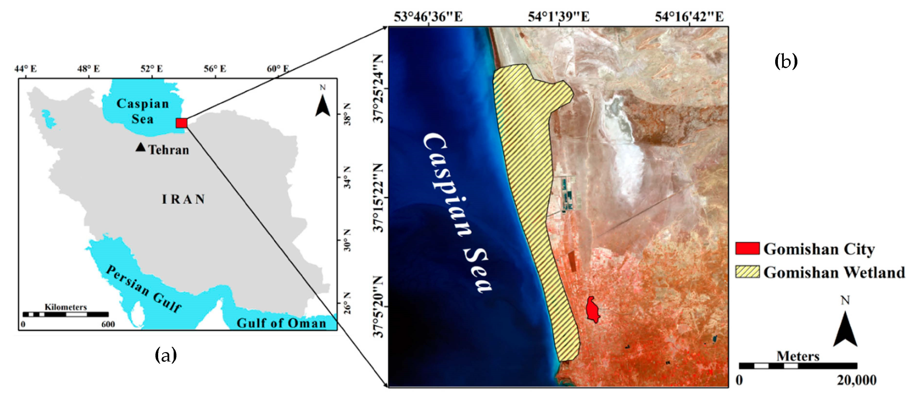
2. Study Area
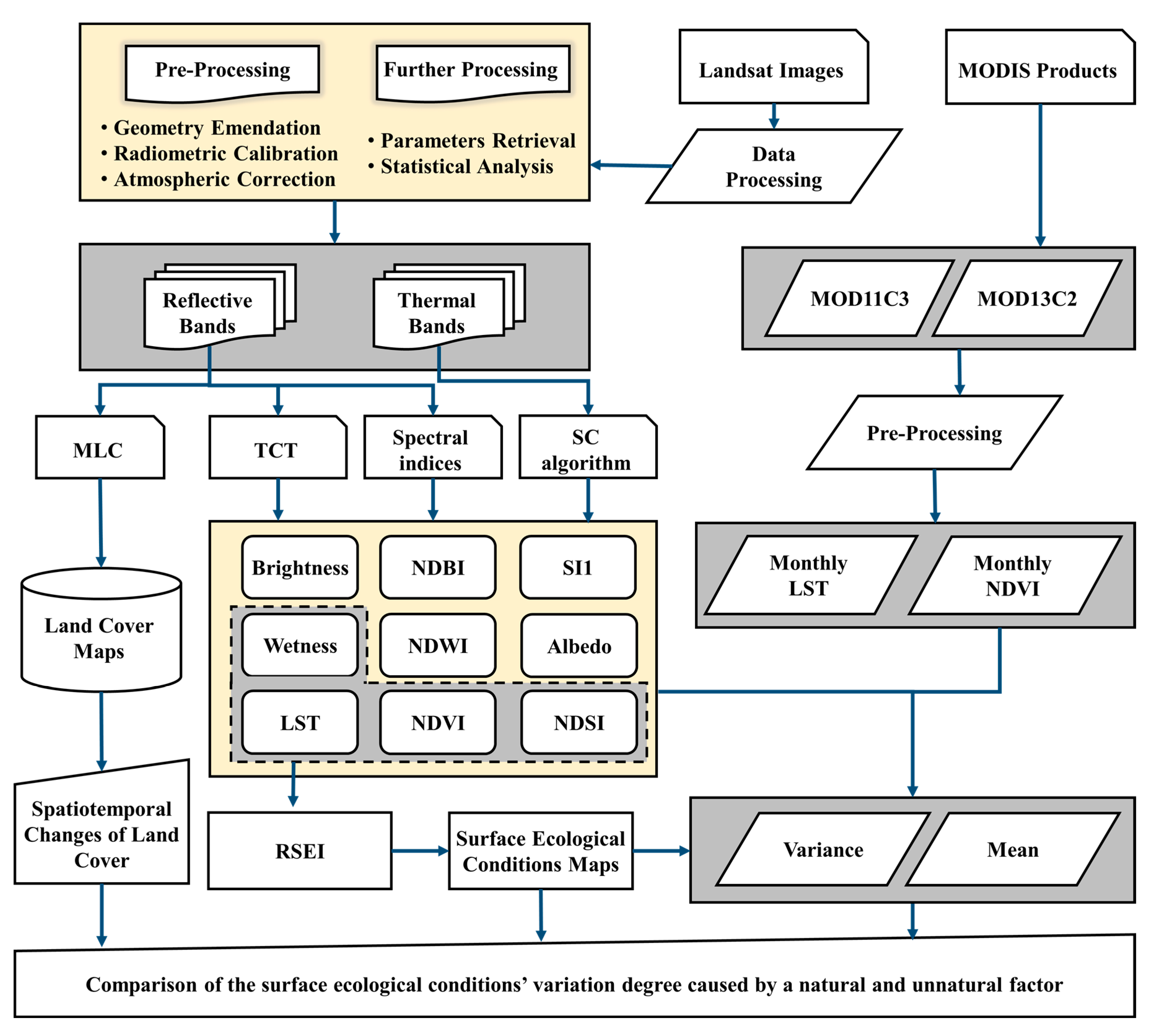
3. Data and Methods
3.1. Data
3.2. Methods
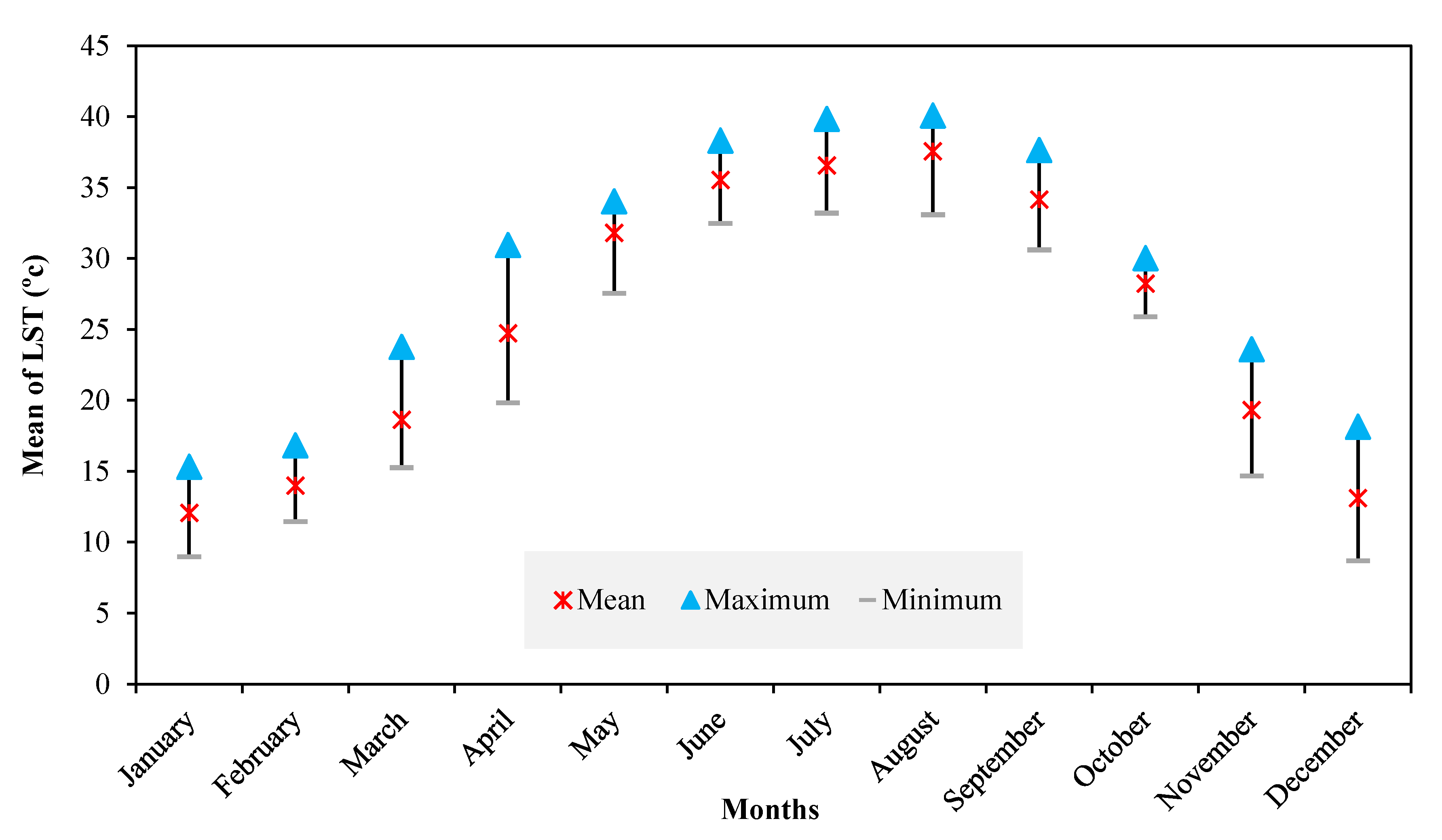
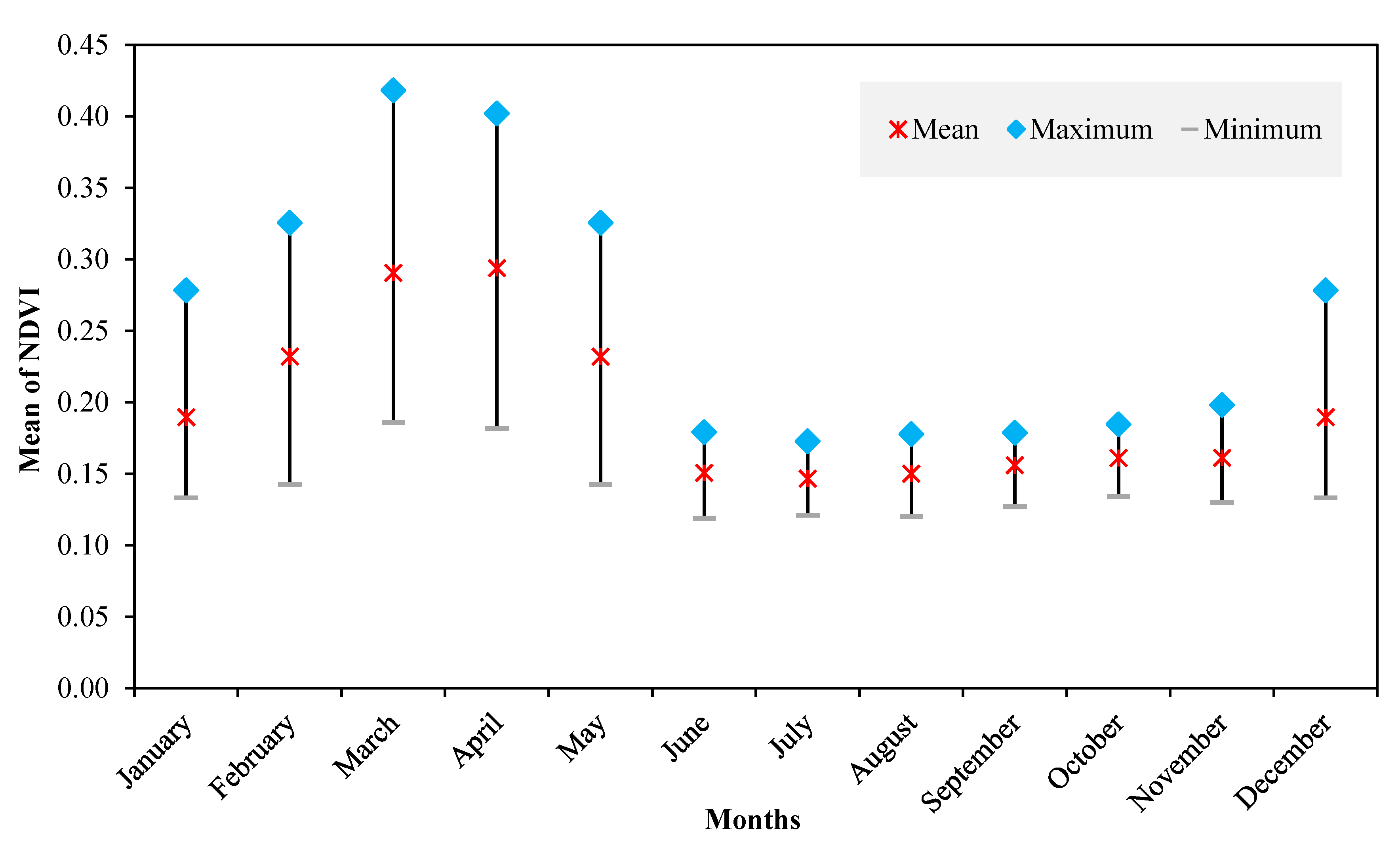
3.2.1. Spatiotemporal Changes of LST and NDVI Using MODIS Products
3.2.2. Spatiotemporal Changes of Surface Biophysical Characteristics Using Landsat Imagery
Extraction of Surface Biophysical Characteristics from Landsat Images
3.2.3. Land Cover Classification
3.2.4. Modeling the Surface Ecological Conditions
4. Results
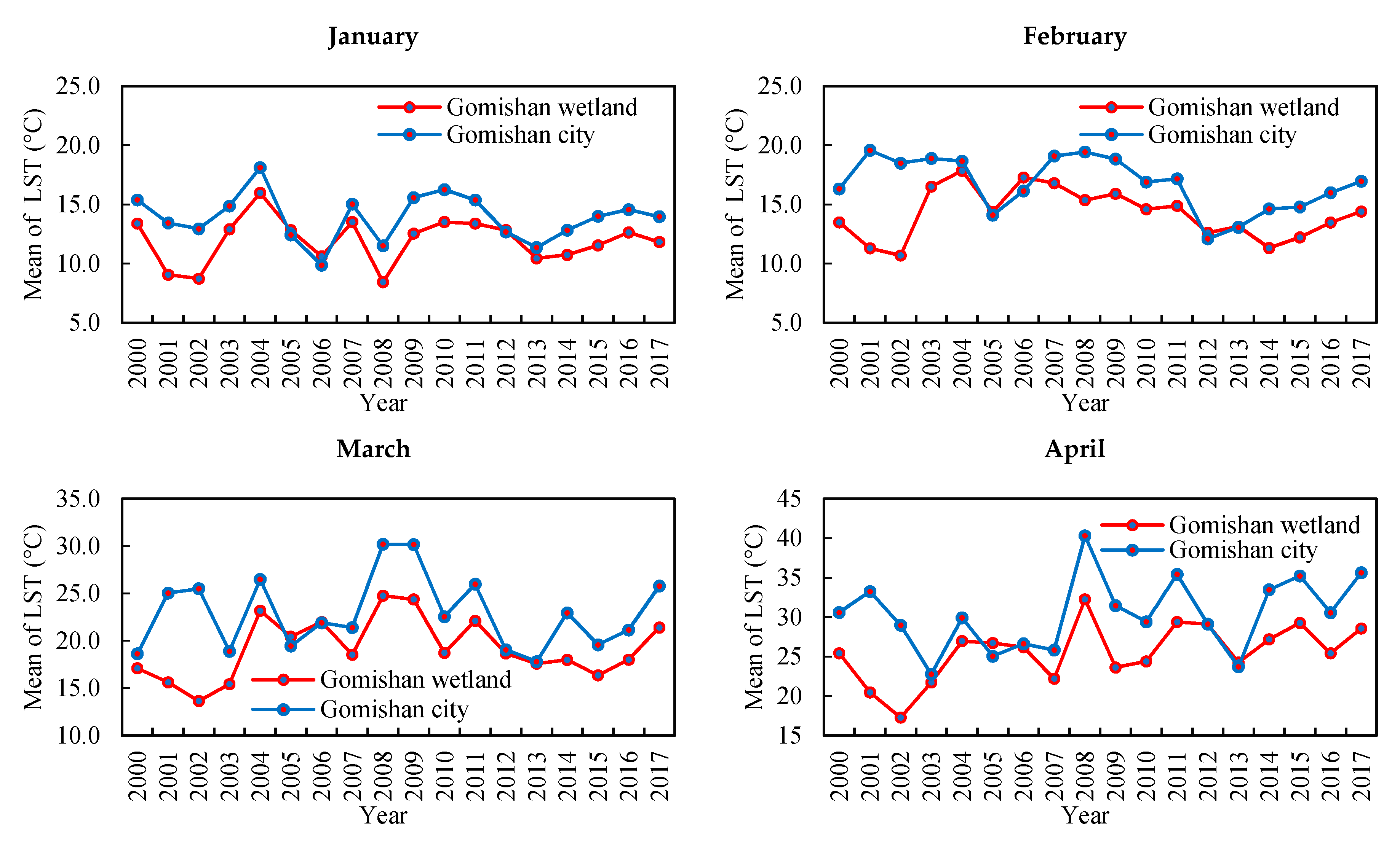
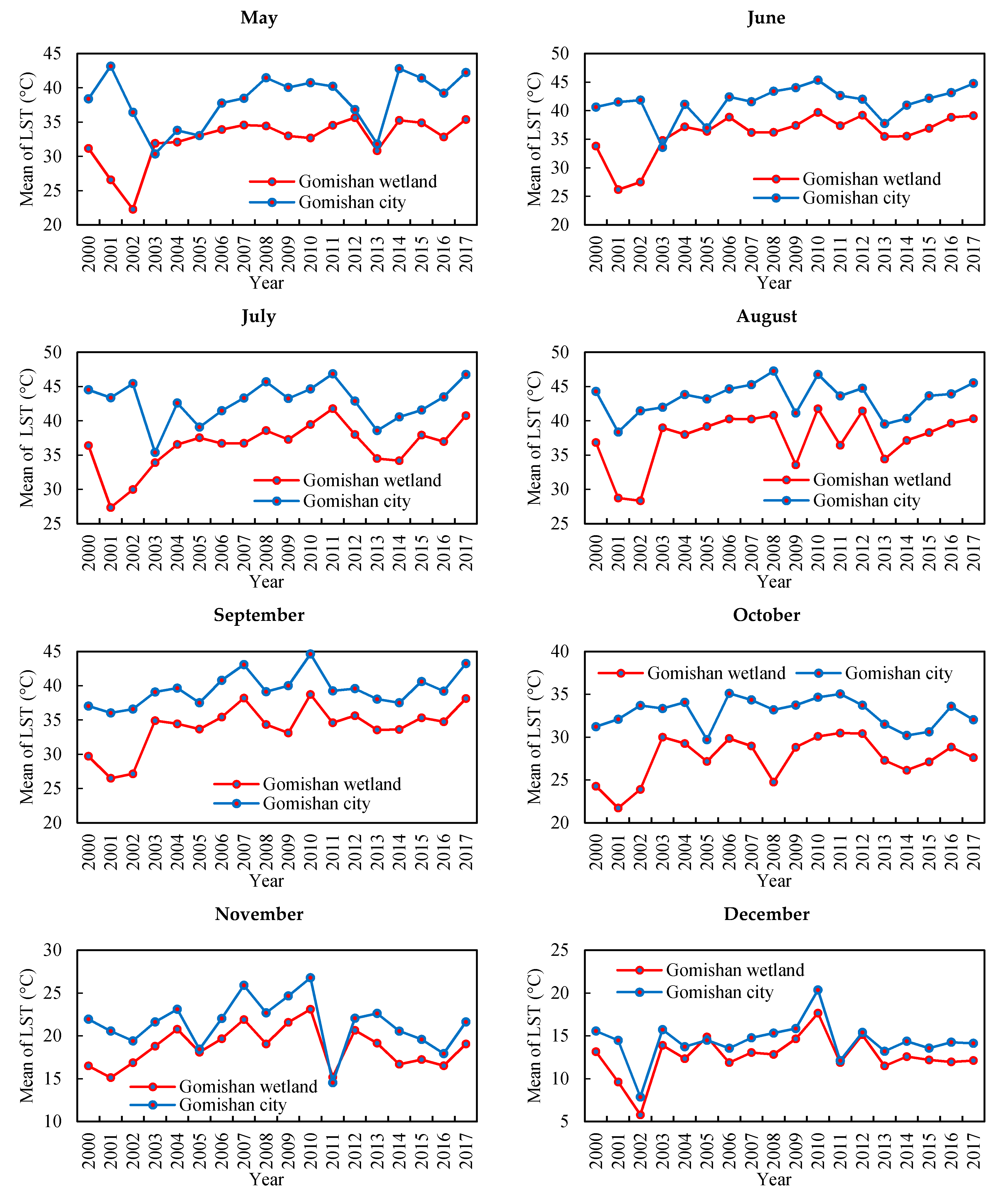
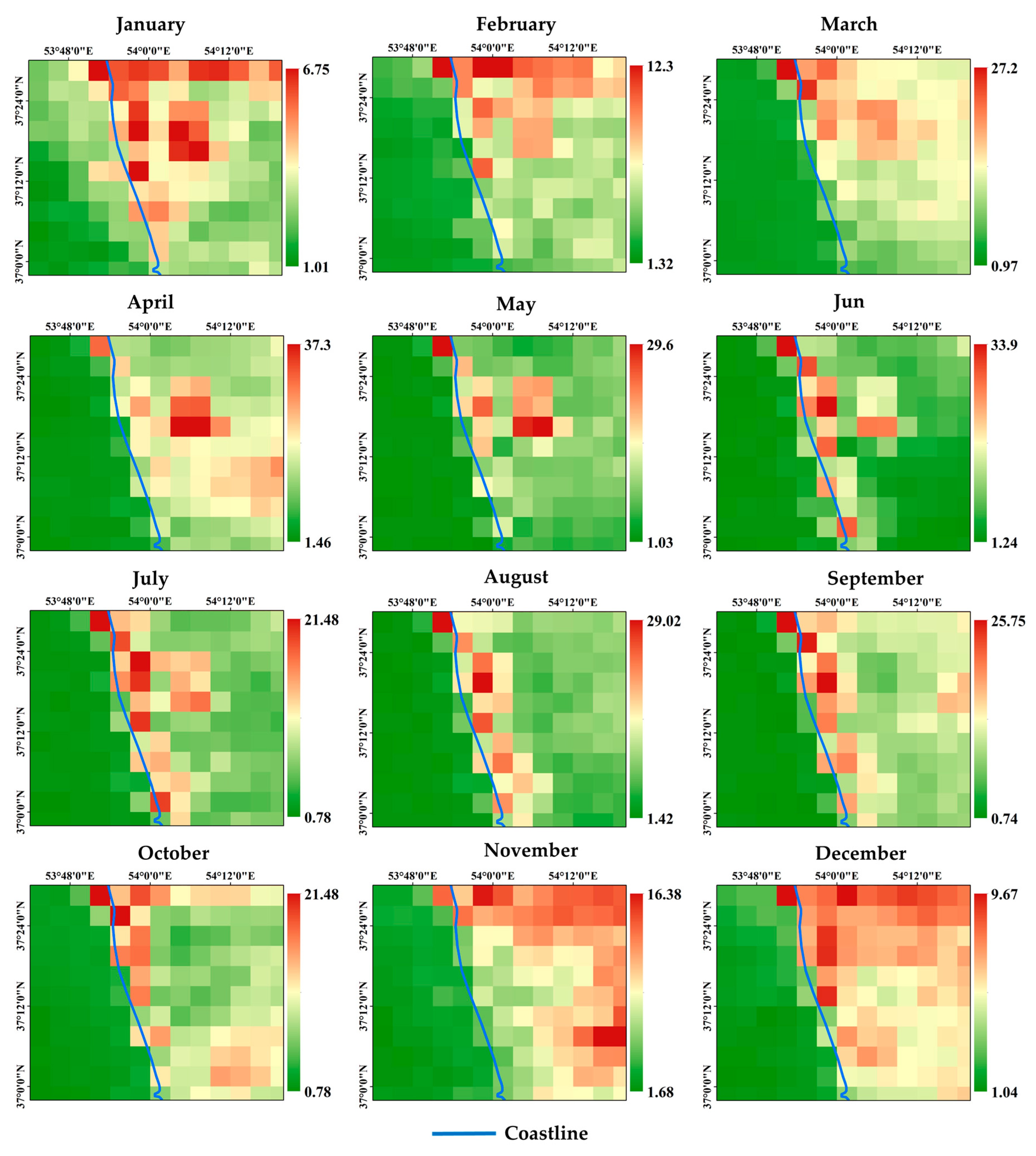
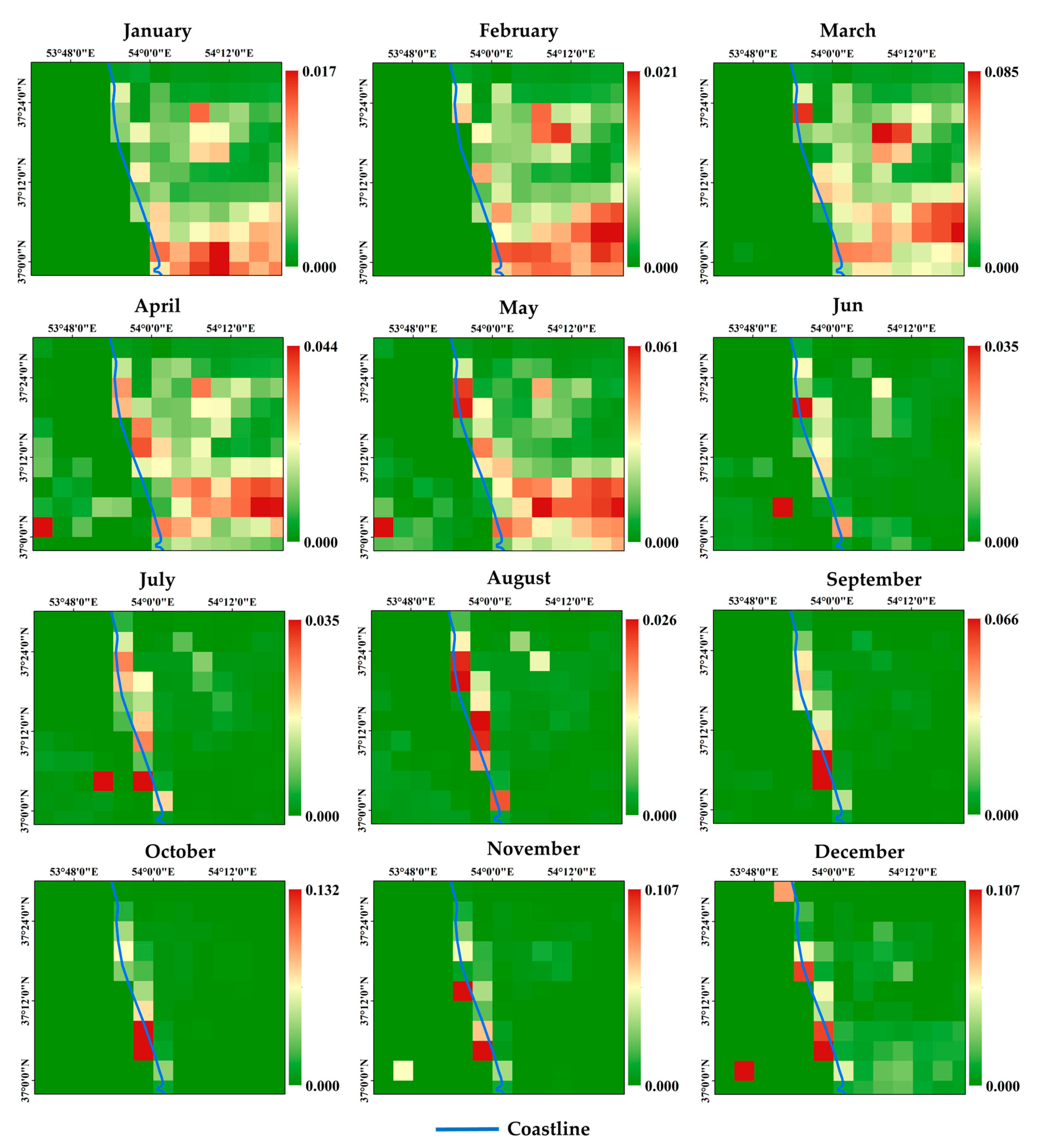
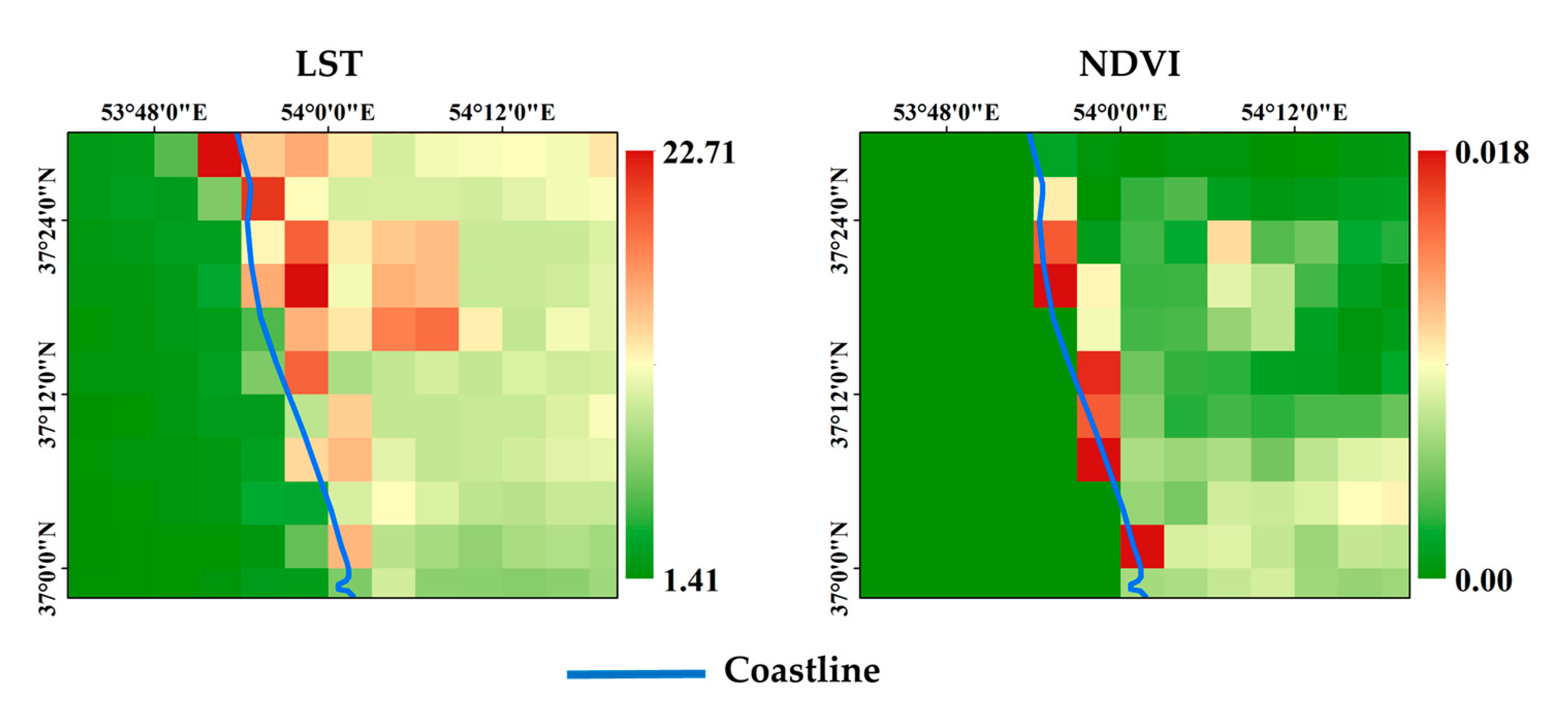
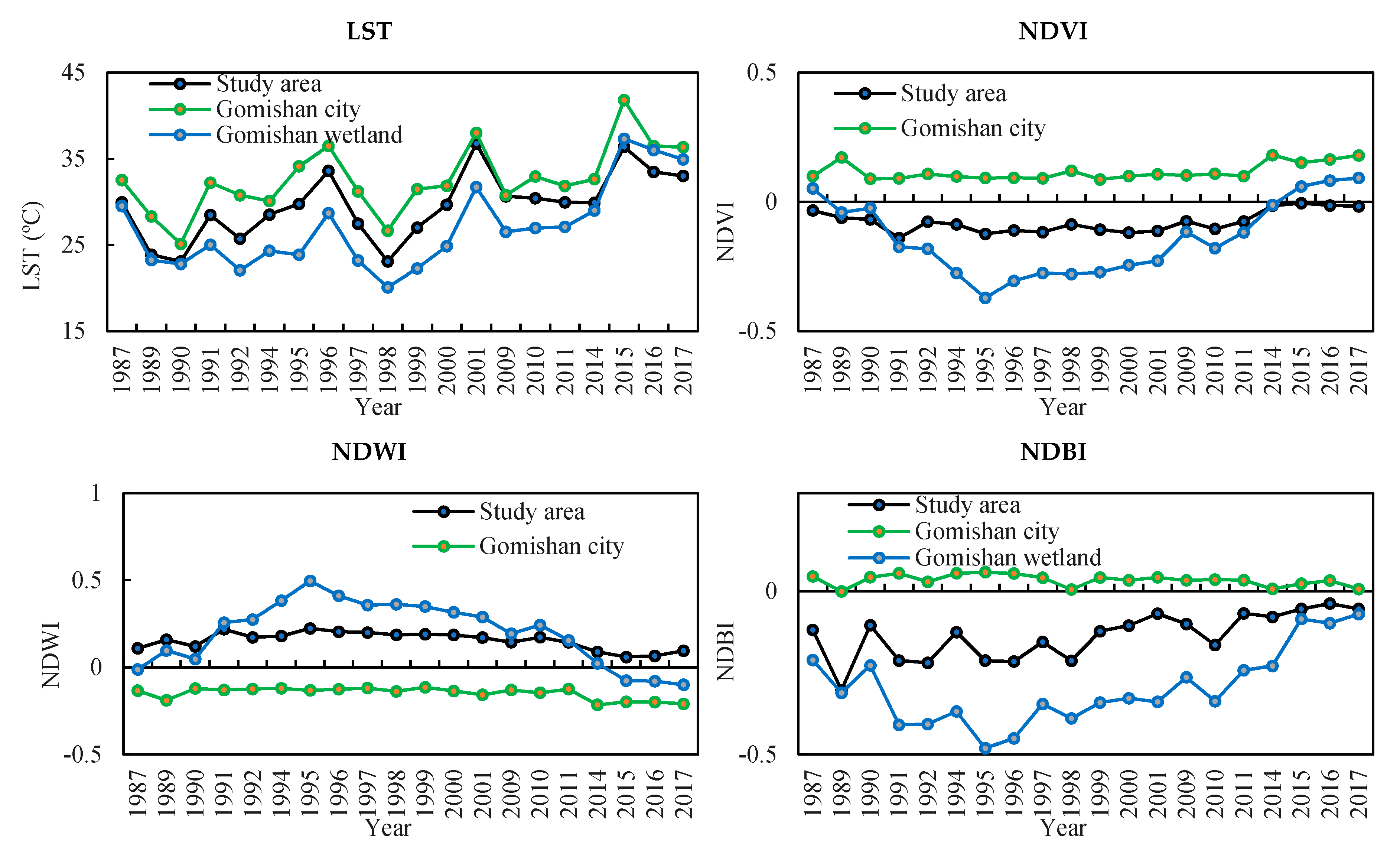
4.1. NDVI and LST Spatiotemporal Variations of the Study Area Using MODIS Products
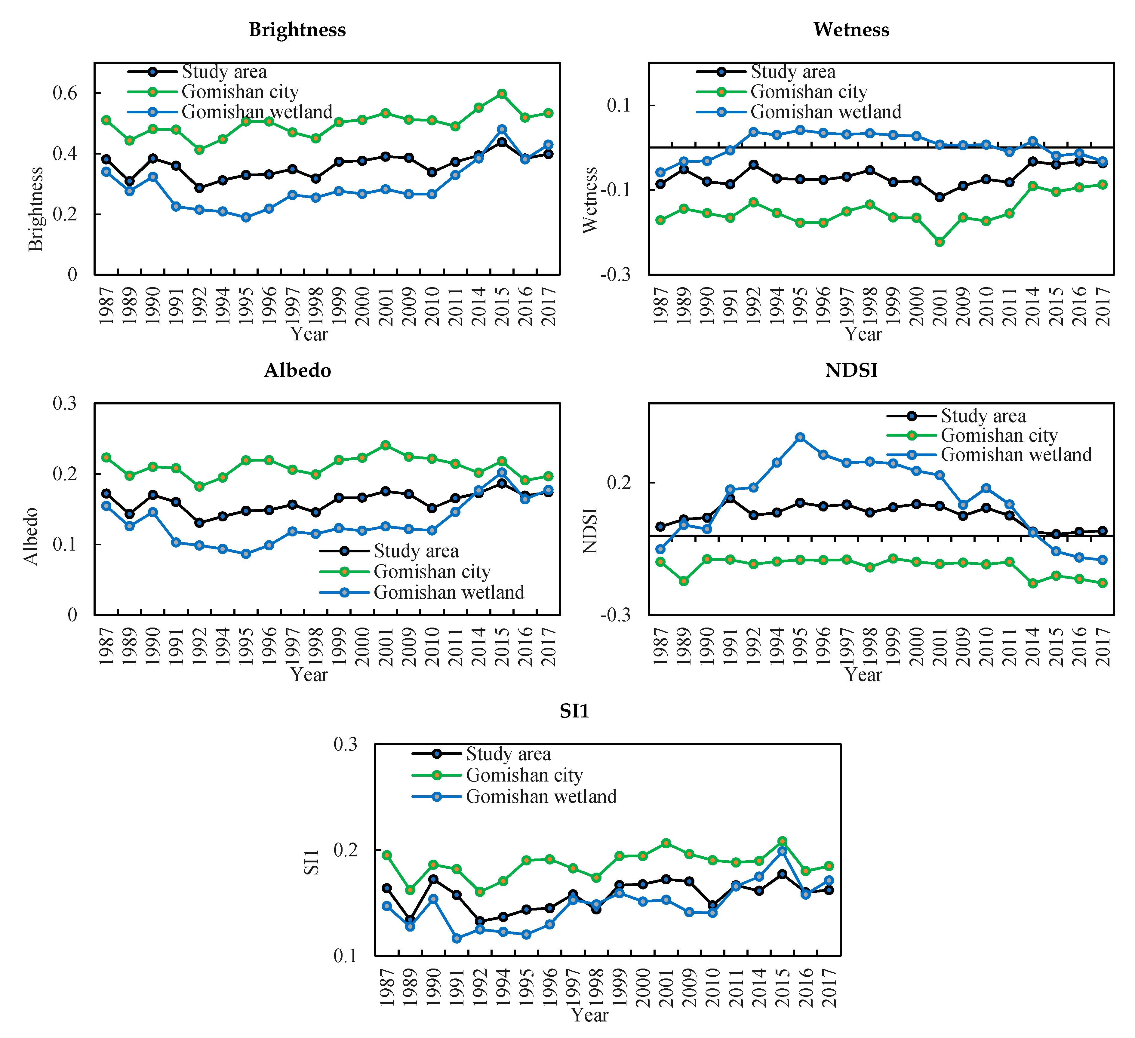
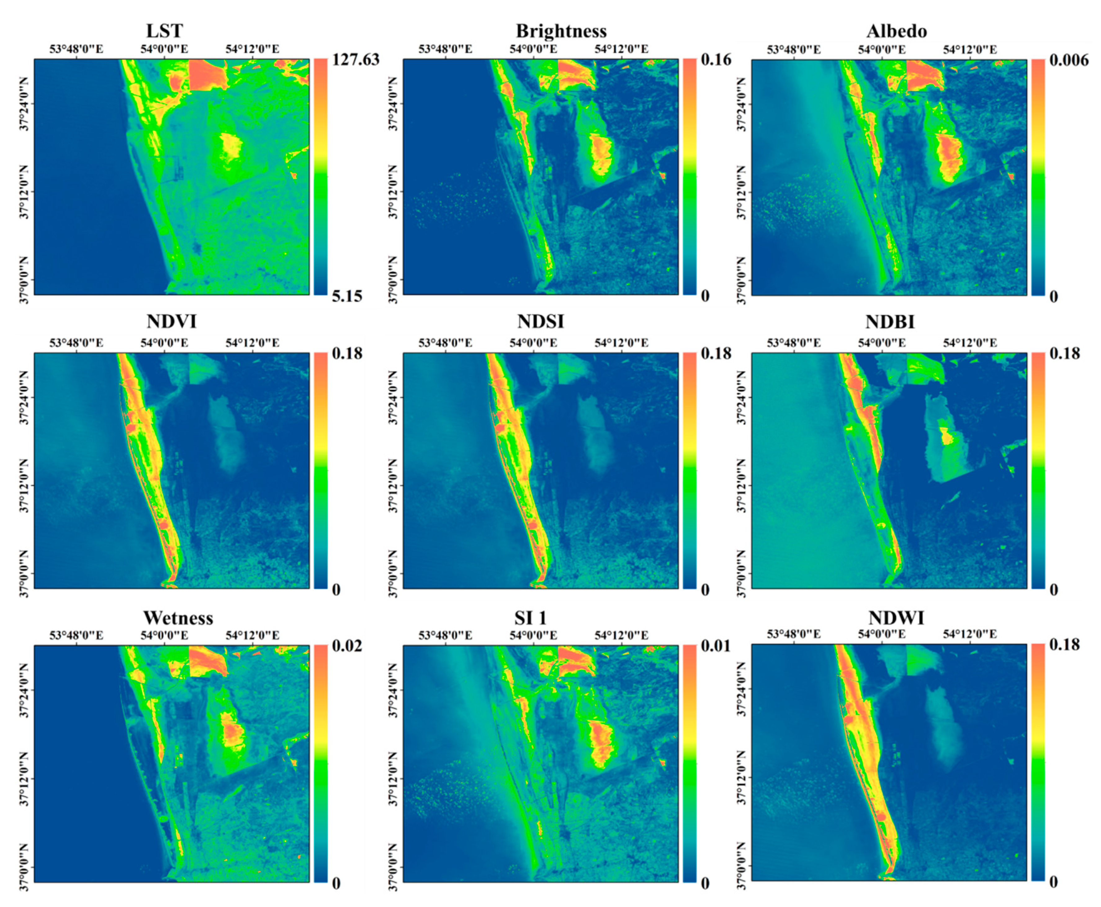
4.2. Spatiotemporal Variations in Biophysical Characteristics Using Landsat Images
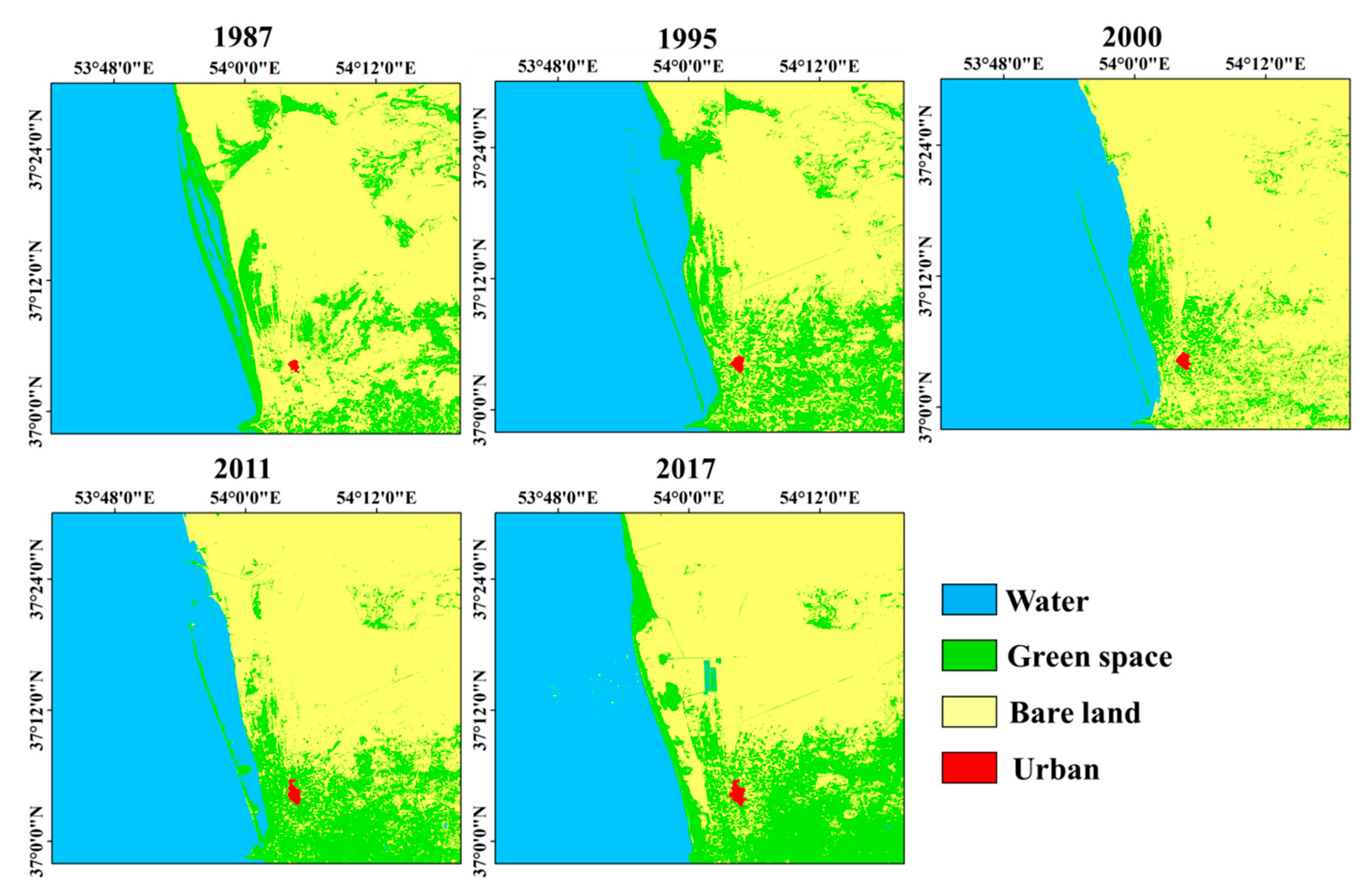
4.3. Land Cover Maps
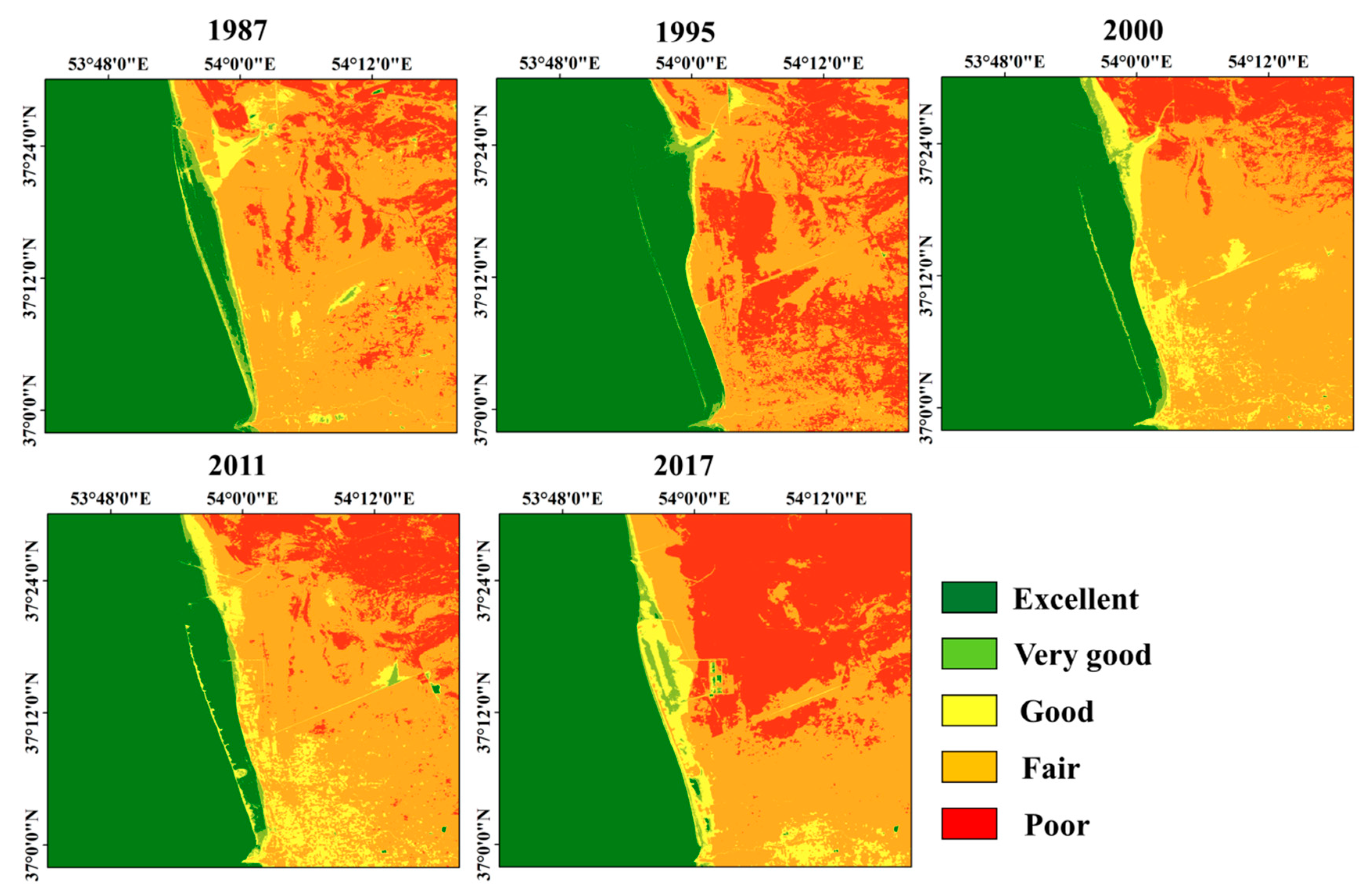
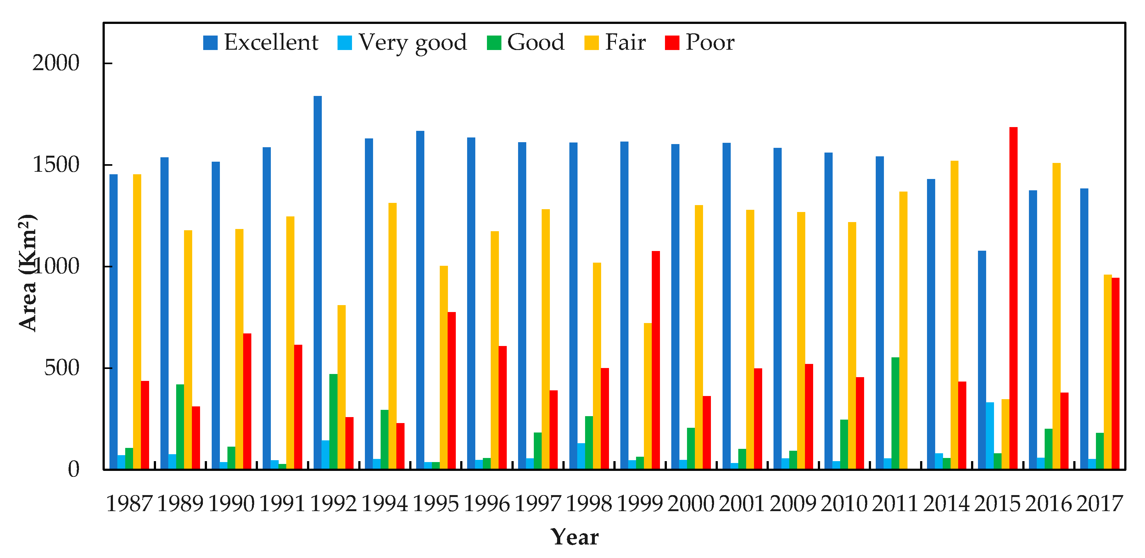
4.4. Spatiotemporal Variations of the Surface Ecological Conditions
5. Discussion
6. Conclusions
Author Contributions
Funding
Acknowledgments
Conflicts of Interest
References
- He, Y.; Xie, H. Exploring the spatiotemporal changes of ecological carrying capacity for regional sustainable development based on GIS: A case study of Nanchang City. Technol. Forecast. Soc. Chang. 2019, 148, 119720. [Google Scholar] [CrossRef]
- Hou, K.; Tao, W.; Wang, L.; Li, X. Study on hierarchical transformation mechanisms of regional ecological vulnerability and its applicability. Ecol. Indic. 2020, 114, 106343. [Google Scholar] [CrossRef]
- Yang, Y.; Meng, G. A bibliometric analysis of comparative research on the evolution of international and Chinese ecological footprint research hotspots and frontiers since 2000. Ecol. Indic. 2019, 102, 650–665. [Google Scholar] [CrossRef]
- Szigeti, C.; Toth, G.; Szabo, D.R. Decoupling–shifts in ecological footprint intensity of nations in the last decade. Ecol. Indic. 2017, 72, 111–117. [Google Scholar] [CrossRef]
- Mijani, N.; Alavipanah, S.K.; Firozjaei, M.K.; Arsanjani, J.J.; Hamzeh, S.; Weng, Q. Modeling outdoor thermal comfort using satellite imagery: A principle component analysis-based approach. Ecol. Indic. 2020, 117, 106555. [Google Scholar] [CrossRef]
- Wang, R.; Li, F.; Hu, D.; Li, B.L. Understanding eco-complexity: Social-economic-natural complex ecosystem approach. Ecol. Complex. 2011, 8, 15–29. [Google Scholar] [CrossRef]
- Larson, K.L.; Nelson, K.C.; Samples, S.; Hall, S.; Bettez, N.; Cavender-Bares, J.; Groffman, P.; Grove, M.; Heffernan, J.; Hobbie, S.E. Ecosystem services in managing residential landscapes: Priorities, value dimensions, and cross-regional patterns. Urban. Ecosyst. 2016, 19, 95–113. [Google Scholar] [CrossRef]
- Xu, C.; Jiang, W.; Huang, Q.; Wang, Y. Ecosystem services response to rural-urban transitions in coastal and island cities: A comparison between Shenzhen and Hong Kong, China. J. Clean. Prod. 2020, 121033. [Google Scholar] [CrossRef]
- Varin, M.; Theau, J.; Fournier, R.A. Mapping ecosystem services provided by wetlands at multiple spatiotemporal scales: A case study in Quebec, Canada. J. Environ. Manag. 2019, 246, 334–344. [Google Scholar] [CrossRef]
- Yuan, Y.; Wu, S.; Yu, Y.; Tong, G.; Mo, L.; Yan, D.; Li, F. Spatiotemporal interaction between ecosystem services and urbanization: Case study of Nanjing City, China. Ecol. Indic. 2018, 95, 917–929. [Google Scholar] [CrossRef]
- Liu, Q.; Wu, J.; Li, L. Ecological environment monitoring for sustainable development goals in the Belt and Road region. J. Remote Sens. 2018, 22, 686–708. [Google Scholar]
- Willis, K.S. Remote sensing change detection for ecological monitoring in United States protected areas. Biol. Conserv. 2015, 182, 233–242. [Google Scholar] [CrossRef]
- Weng, Q. Thermal infrared remote sensing for urban climate and environmental studies: Methods, applications, and trends. ISPRS J. Photogramm. Remote Sens. 2009, 64, 335–344. [Google Scholar] [CrossRef]
- Firozjaei, M.K.; Fathololoumi, S.; Weng, Q.; Kiavarz, M.; Alavipanah, S.K. Remotely Sensed Urban Surface Ecological Index (RSUSEI): An Analytical Framework for Assessing the Surface Ecological Status in Urban Environments. Remote Sens. 2020, 12, 2029. [Google Scholar] [CrossRef]
- Hu, X.; Xu, H. A new remote sensing index for assessing the spatial heterogeneity in urban ecological quality: A case from Fuzhou City, China. Ecol. Indic. 2018, 89, 11–21. [Google Scholar] [CrossRef]
- de Araujo Barbosa, C.C.; Atkinson, P.M.; Dearing, J.A. Remote sensing of ecosystem services: A systematic review. Ecol. Indic. 2015, 52, 430–443. [Google Scholar] [CrossRef]
- Reza, M.I.H.; Abdullah, S.A. Regional Index of Ecological Integrity: A need for sustainable management of natural resources. Ecol. Indic. 2011, 11, 220–229. [Google Scholar] [CrossRef]
- Kennedy, R.E.; Andréfouët, S.; Cohen, W.B.; Gómez, C.; Griffiths, P.; Hais, M.; Healey, S.P.; Helmer, E.H.; Hostert, P.; Lyons, M.B. Bringing an ecological view of change to Landsat-based remote sensing. Front. Ecol. Environ. 2014, 12, 339–346. [Google Scholar] [CrossRef]
- Firozjaei, M.K.; Weng, Q.; Zhao, C.; Kiavarz, M.; Lu, L.; Alavipanah, S.K. Surface anthropogenic heat islands in six megacities: An assessment based on a triple-source surface energy balance model. Remote Sens. Environ. 2020, 242, 111751. [Google Scholar] [CrossRef]
- Wu, J.; Wang, X.; Zhong, B.; Yang, A.; Jue, K.; Wu, J.; Zhang, L.; Xu, W.; Wu, S.; Zhang, N. Ecological environment assessment for Greater Mekong Subregion based on Pressure-State-Response framework by remote sensing. Ecol. Indic. 2020, 117, 106521. [Google Scholar] [CrossRef]
- White, D.C.; Lewis, M.M.; Green, G.; Gotch, T.B. A generalizable NDVI-based wetland delineation indicator for remote monitoring of groundwater flows in the Australian Great Artesian Basin. Ecol. Indic. 2016, 60, 1309–1320. [Google Scholar] [CrossRef]
- Coutts, A.M.; Harris, R.J.; Phan, T.; Livesley, S.J.; Williams, N.S.; Tapper, N.J. Thermal infrared remote sensing of urban heat: Hotspots, vegetation, and an assessment of techniques for use in urban planning. Remote Sens. Environ. 2016, 186, 637–651. [Google Scholar] [CrossRef]
- Ochoa-Gaona, S.; Kampichler, C.; De Jong, B.; Hernández, S.; Geissen, V.; Huerta, E. A multi-criterion index for the evaluation of local tropical forest conditions in Mexico. For. Ecol. Manag. 2010, 260, 618–627. [Google Scholar] [CrossRef]
- Nichol, J. An emissivity modulation method for spatial enhancement of thermal satellite images in urban heat island analysis. Photogramm. Eng. Remote Sens. 2009, 75, 547–556. [Google Scholar] [CrossRef]
- Yue, H.; Liu, Y.; Li, Y.; Lu, Y. Eco-environmental quality assessment in China’s 35 major cities based on remote sensing ecological index. IEEE Access 2019, 7, 51295–51311. [Google Scholar] [CrossRef]
- Xu, H.; Wang, M.; Shi, T.; Guan, H.; Fang, C.; Lin, Z. Prediction of ecological effects of potential population and impervious surface increases using a remote sensing based ecological index (RSEI). Ecol. Indic. 2018, 93, 730–740. [Google Scholar] [CrossRef]
- Zhang, J.; Zhu, Y.; Fan, F. Mapping and evaluation of landscape ecological status using geographic indices extracted from remote sensing imagery of the Pearl River Delta, China, between 1998 and 2008. Environ. Earth Sci. 2016, 75, 327. [Google Scholar] [CrossRef]
- Li, J.; Song, C.; Cao, L.; Zhu, F.; Meng, X.; Wu, J. Impacts of landscape structure on surface urban heat islands: A case study of Shanghai, China. Remote Sens. Environ. 2011, 115, 3249–3263. [Google Scholar] [CrossRef]
- Buyantuyev, A.; Wu, J. Urban heat islands and landscape heterogeneity: Linking spatiotemporal variations in surface temperatures to land-cover and socioeconomic patterns. Landsc. Ecol. 2010, 25, 17–33. [Google Scholar] [CrossRef]
- Fu, Y.; Shi, X.; He, J.; Yuan, Y.; Qu, L. Identification and optimization strategy of county ecological security pattern: A case study in the Loess Plateau, China. Ecol. Indic. 2020, 112, 106030. [Google Scholar] [CrossRef]
- Ouyang, Z.; Wang, Q.; Zheng, H.; Zhang, F.; Hou, P. National ecosystem survey and assessment of China (2000–2010). Bull. Chin. Acad. Sci. 2014, 29, 462–466. [Google Scholar]
- Guan, Q.; Hao, J.; Ren, G.; Li, M.; Chen, A.; Duan, W.; Chen, H. Ecological indexes for the analysis of the spatial–temporal characteristics of ecosystem service supply and demand: A case study of the major grain-producing regions in Quzhou, China. Ecol. Indic. 2020, 108, 105748. [Google Scholar] [CrossRef]
- Shan, W.; Jin, X.; Ren, J.; Wang, Y.; Xu, Z.; Fan, Y.; Gu, Z.; Hong, C.; Lin, J.; Zhou, Y. Ecological environment quality assessment based on remote sensing data for land consolidation. J. Clean. Prod. 2019, 239, 118126. [Google Scholar] [CrossRef]
- Yang, C.; Zhang, C.; Li, Q.; Liu, H.; Gao, W.; Shi, T.; Liu, X.; Wu, G. Rapid urbanization and policy variation greatly drive ecological quality evolution in Guangdong-Hong Kong-Macau Greater Bay Area of China: A remote sensing perspective. Ecol. Indic. 2020, 115, 106373. [Google Scholar] [CrossRef]
- Chen, X.; Li, F.; Li, X.; Hu, Y.; Wang, Y. Mapping ecological space quality changes for ecological management: A case study in the Pearl River Delta urban agglomeration, China. J. Environ. Manag. 2020, 267, 110658. [Google Scholar] [CrossRef]
- Shen, G.; Yang, X.; Jin, Y.; Xu, B.; Zhou, Q. Remote sensing and evaluation of the wetland ecological degradation process of the Zoige Plateau Wetland in China. Ecol. Indic. 2019, 104, 48–58. [Google Scholar] [CrossRef]
- Eid, A.N.M.; Olatubara, C.; Ewemoje, T.; El-Hennawy, M.T.; Farouk, H. Inland wetland time-series digital change detection based on SAVI and NDWI indecies: Wadi El-Rayan lakes, Egypt. Remote Sens. Appl. Soc. Environ. 2020, 19, 100347. [Google Scholar] [CrossRef]
- Rapinel, S.; Fabre, E.; Dufour, S.; Arvor, D.; Mony, C.; Hubert-Moy, L. Mapping potential, existing and efficient wetlands using free remote sensing data. J. Environ. Manag. 2019, 247, 829–839. [Google Scholar] [CrossRef]
- Singh, S.; Bhardwaj, A.; Verma, V. Remote sensing and GIS based analysis of temporal land use/land cover and water quality changes in Harike wetland ecosystem, Punjab, India. J. Environ. Manag. 2020, 262, 110355. [Google Scholar] [CrossRef]
- Orimoloye, I.R.; Mazinyo, S.P.; Kalumba, A.; Nel, W.; Adigun, A.I.; Ololade, O.O. Wetland shift monitoring using remote sensing and GIS techniques: Landscape dynamics and its implications on Isimangaliso Wetland Park, South Africa. Earth Sci. Inform. 2019, 12, 553–563. [Google Scholar] [CrossRef]
- Alavipanah, S.; Konyushkova, M.; Hamzeh, S.; Kakroodi, A.; Heidari, A.; Firozjaei, M.; Mijani, N. Characterizing Spatial and Temporal Trends of Soil and Surface Properties Changes in AN Area with Urban, Bare Soil and Wetland Covers: A 30-YEAR Case Study in Gomishan, Iran. Int. Arch. Photogramm. Remote Sens. Spat. Inf. Sci. 2019, 42, 51–56. [Google Scholar] [CrossRef]
- Emberger, L. Sur une formule climatique et ses applications en botanique. La Météorol. 1932, 92, 1–10. [Google Scholar]
- Jeihouni, M.; Kakroodi, A.; Hamzeh, S. Monitoring shallow coastal environment using Landsat/altimetry data under rapid sea-level change. Estuar. Coast. Shelf Sci. 2019, 224, 260–271. [Google Scholar] [CrossRef]
- Bodart, C.; Eva, H.; Beuchle, R.; Raši, R.; Simonetti, D.; Stibig, H.-J.; Brink, A.; Lindquist, E.; Achard, F. Pre-processing of a sample of multi-scene and multi-date Landsat imagery used to monitor forest cover changes over the tropics. ISPRS J. Photogramm. Remote Sens. 2011, 66, 555–563. [Google Scholar] [CrossRef]
- Bruce, C.M.; Hilbert, D.W. Pre-Processing Methodology for Application to Landsat TM/ETM+ Imagery of the Wet Tropics; Rainforest CRC: Cairns, Australia, 2006. [Google Scholar]
- Phiri, D.; Morgenroth, J.; Xu, C.; Hermosilla, T. Effects of pre-processing methods on Landsat OLI-8 land cover classification using OBIA and random forests classifier. Int. J. Appl. Earth Obs. Geoinf. 2018, 73, 170–178. [Google Scholar] [CrossRef]
- Tucker, C.J. Red and photographic infrared linear combinations for monitoring vegetation. Remote Sens. Environ. 1979, 8, 127–150. [Google Scholar] [CrossRef]
- Allbed, A.; Kumar, L. Soil salinity mapping and monitoring in arid and semi-arid regions using remote sensing technology: A review. Adv. Remote Sens. 2013, 2013. [Google Scholar] [CrossRef]
- Zha, Y.; Gao, J.; Ni, S. Use of normalized difference built-up index in automatically mapping urban areas from TM imagery. Int. J. Remote Sens. 2003, 24, 583–594. [Google Scholar] [CrossRef]
- Gao, B.C. NDWI-A normalized difference water index for remote sensing of vegetation liquid water from space. Remote Sens. Environ. 1996, 58, 257–266. [Google Scholar] [CrossRef]
- Taleghani, M. The impact of increasing urban surface albedo on outdoor summer thermal comfort within a university campus. Urban. Clim. 2018, 24, 175–184. [Google Scholar] [CrossRef]
- Liu, Q.; Liu, G.; Huang, C.; Liu, S.; Zhao, J. A tasseled cap transformation for Landsat 8 OLI TOA reflectance images. In Proceedings of the Geoscience and Remote Sensing Symposium (IGARSS) 2014 IEEE International, Quebec, QC, Canada, 13–18 July 2014; pp. 541–544. [Google Scholar]
- Liu, Q.; Liu, G.; Huang, C.; Xie, C. Comparison of tasselled cap transformations based on the selective bands of Landsat 8 OLI TOA reflectance images. Int. J. Remote Sens. 2015, 36, 417–441. [Google Scholar] [CrossRef]
- Jiménez-Muñoz, J.C.; Sobrino, J.A. A generalized single-channel method for retrieving land surface temperature from remote sensing data. J. Geophys. Res. Atmos. 2003, 108, 4688. [Google Scholar] [CrossRef]
- Firozjaei, M.K.; Kiavarz, M.; Alavipanah, S.K.; Lakes, T.; Qureshi, S. Monitoring and forecasting heat island intensity through multi-temporal image analysis and cellular automata-Markov chain modelling: A case of Babol city, Iran. Ecol. Indic. 2018, 91, 155–170. [Google Scholar] [CrossRef]
- Weng, Q.; Firozjaei, M.K.; Sedighi, A.; Kiavarz, M.; Alavipanah, S.K. Statistical analysis of surface urban heat island intensity variations: A case study of Babol city, Iran. GISci. Remote Sens. 2018, 1–29. [Google Scholar] [CrossRef]
- Otukei, J.R.; Blaschke, T. Land cover change assessment using decision trees, support vector machines and maximum likelihood classification algorithms. Int. J. Appl. Earth Obs. Geoinf. 2010, 12, S27–S31. [Google Scholar] [CrossRef]
- Moghaddam, M.H.R.; Sedighi, A.; Fasihi, S.; Firozjaei, M.K. Effect of environmental policies in combating aeolian desertification over Sejzy Plain of Iran. Aeolian Res. 2018, 35, 19–28. [Google Scholar] [CrossRef]
- Xu, H.; Wang, Y.; Guan, H.; Shi, T.; Hu, X. Detecting Ecological Changes with a Remote Sensing Based Ecological Index (RSEI) Produced Time Series and Change Vector Analysis. Remote Sens. 2019, 11, 2345. [Google Scholar] [CrossRef]


| Satellite (Sensor) | Product | Acquisition Date | Temporal Resolution | Spatial Resolution (m) | Source |
|---|---|---|---|---|---|
| Landsat 5 (TM/TIR) | L1T | 14/06/1987, 02/05/1989, 21/05/1990, 09/06/1991, 11/06/1992, 03/07/1994, 20/06/1995, 24/07/1996, 24/05/1997, 11/05/1998, 30/05/1999, 17/06/2000, 26/06/2009, 28/05/2010 and 31/05/2011 | 16-day | 30 (120) | USGS Earth Explorer |
| Landsat 7 (ETM+/TIR) | 30/07/2001 | 30 (60) | |||
| Landsat 8 (OLI/TIRS) | 07/05/2014, 26/05/2015, 28/05/2016 and 15/05/2017 | 30 (100) | |||
| Terra (MODIS) | MOD13C3 | 2000–2017 | Monthly | 5000 | LAADS Explorer |
| MOD11C3 | 2000–2017 |
| Parameters | Description | Equation | Reference |
|---|---|---|---|
| Normalized Difference Vegetation Index (NDVI) | Indicates vegetation cover information. | [47] | |
| Normalized Difference Salinity Index (NDSI) | Indicates surface salinity information. | [48] | |
| Normalized Difference Built-up Index (NDBI) | Indicates impervious surface, bare and built-up land information | [49] | |
| Normalized Difference Water Index (NDWI) | Indicates moisture information including soil moisture, water-related complications, built-up land and plant | [50] | |
| Albedo | One of the important and effective factors on the energy parameters balance, temperature and evaporation and surface transpiration, which depends on the type and absorption of solar radiation. | [51] | |
| Brightness | First components of Tasseled Cap Transformation (TCT), indicates information on the percentage of impermeable surfaces including bare and constructed land | [52,53] | |
| Wetness | Third components of Tasseled Cap Transformation (TCT), indicates the characteristics of water, soil, plant and constructed lands related effects | ||
| Land Surface Temperature (LST) | LST is one of the important parameters for controlling and evaluating the biological, chemical and physical processes of the Earth’s surface and is an important factor for studying the Earth’s ecological conditions and land resource management activities. | [54,55,56] | |
| Salinity Index 1 (SI1) | Indicates the salt affected lands with sparse vegetation cover | [48] |
| Parameter | LST (°C) | NDVI | NDBI | NDWI | Brightness | Wetness | Albedo | NDSI | SI 1 |
|---|---|---|---|---|---|---|---|---|---|
| Study area | 21.5 | 0.009 | 0.018 | 0.011 | 0.004 | 0.002 | 0.001 | 0.009 | 0.001 |
| City | 15.3 | 0.002 | 0.001 | 0.002 | 0.003 | 0.001 | 0.001 | 0.002 | 0.001 |
| Talab | 30.9 | 0.060 | 0.048 | 0.055 | 0.011 | 0.003 | 0.002 | 0.041 | 0.002 |
| Year | Urban | Green Space | Bare Soil | Water |
|---|---|---|---|---|
| 1987 | 2.15 | 489.79 | 1606.94 | 1419.52 |
| 1989 | 2.29 | 552.51 | 1438.60 | 1525.00 |
| 1990 | 2.36 | 643.27 | 1369.90 | 1502.88 |
| 1991 | 2.48 | 700.46 | 1283.61 | 1531.85 |
| 1992 | 2.61 | 715.86 | 1031.44 | 1768.49 |
| 1994 | 2.95 | 323.34 | 1584.69 | 1607.41 |
| 1995 | 3.1 | 556.00 | 1321.59 | 1637.71 |
| 1996 | 3.35 | 210.66 | 1691.10 | 1613.29 |
| 1997 | 3.51 | 540.01 | 1368.59 | 1606.29 |
| 1998 | 3.7 | 468.05 | 1432.32 | 1614.33 |
| 1999 | 3.9 | 349.04 | 1554.36 | 1611.09 |
| 2000 | 4.05 | 240.14 | 1664.88 | 1609.33 |
| 2001 | 4.18 | 251.89 | 1672.63 | 1589.70 |
| 2009 | 4.8 | 250.61 | 1709.68 | 1553.31 |
| 2010 | 4.9 | 557.62 | 1385.16 | 1570.72 |
| 2011 | 5.05 | 454.50 | 1500.03 | 1558.82 |
| 2014 | 5.9 | 486.44 | 1518.17 | 1507.90 |
| 2015 | 6.16 | 495.93 | 1619.31 | 1397.00 |
| 2016 | 6.29 | 598.74 | 1547.50 | 1365.86 |
| 2017 | 6.48 | 507.13 | 1614.41 | 1390.38 |
© 2020 by the authors. Licensee MDPI, Basel, Switzerland. This article is an open access article distributed under the terms and conditions of the Creative Commons Attribution (CC BY) license (http://creativecommons.org/licenses/by/4.0/).
Share and Cite
Qureshi, S.; Alavipanah, S.K.; Konyushkova, M.; Mijani, N.; Fathololomi, S.; Firozjaei, M.K.; Homaee, M.; Hamzeh, S.; Kakroodi, A.A. A Remotely Sensed Assessment of Surface Ecological Change over the Gomishan Wetland, Iran. Remote Sens. 2020, 12, 2989. https://doi.org/10.3390/rs12182989
Qureshi S, Alavipanah SK, Konyushkova M, Mijani N, Fathololomi S, Firozjaei MK, Homaee M, Hamzeh S, Kakroodi AA. A Remotely Sensed Assessment of Surface Ecological Change over the Gomishan Wetland, Iran. Remote Sensing. 2020; 12(18):2989. https://doi.org/10.3390/rs12182989
Chicago/Turabian StyleQureshi, Salman, Seyed Kazem Alavipanah, Maria Konyushkova, Naeim Mijani, Solmaz Fathololomi, Mohammad Karimi Firozjaei, Mehdi Homaee, Saeid Hamzeh, and Ata Abdollahi Kakroodi. 2020. "A Remotely Sensed Assessment of Surface Ecological Change over the Gomishan Wetland, Iran" Remote Sensing 12, no. 18: 2989. https://doi.org/10.3390/rs12182989
APA StyleQureshi, S., Alavipanah, S. K., Konyushkova, M., Mijani, N., Fathololomi, S., Firozjaei, M. K., Homaee, M., Hamzeh, S., & Kakroodi, A. A. (2020). A Remotely Sensed Assessment of Surface Ecological Change over the Gomishan Wetland, Iran. Remote Sensing, 12(18), 2989. https://doi.org/10.3390/rs12182989